A Posteriori Error Analysis of Mixed Finite Element Methods for Coupled Brinkman–Forchheimer and Double-Diffusion Equations

A posteriori error analysis of a mixed finite element method for the coupled Brinkman–Forchheimer and double-diffusion equations

Sergio Caucao^† Gabriel N. Gatica^‡ Ricardo Oyarz´ua^§ Paulo Z´u˜niga^¶

Abstract

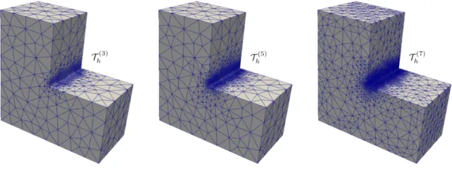
In this paper we consider a partially augmented fully-mixed variational formulation that has been recently proposed for the coupling of the stationary Brinkman–Forchheimer and double-diffusion equations, and develop an a posteriorierror analysis for the 2D and 3D versions of the associated mixed finite element scheme. Indeed, we derive two reliable and efficient residual-baseda posteriori error estimators for this problem on arbitrary (convex or non-convex) polygonal and polyhedral regions. The reliability of the proposed estimators draws mainly upon the uniform ellipticity and inf-sup condition of the forms involved, a suitable assumption on the data, stable Helmholtz decompositions in Hilbert and Banach frameworks, and the local approximation properties of the Cl´ement and Raviart–Thomas operators. In turn, inverse inequalities, the localization technique based on bubble functions, and known results from previous works, are the main tools yielding the efficiency estimate. Finally, several numerical examples confirming the theoretical properties of the estimators and illustrating the performance of the associated adaptive algorithms, are reported. In particular, the case of flow through a 3D porous media with channel networks is considered.

Key words: Brinkman–Forchheimer equations, double-diffusion equations, stress-velocity formula- tion, mixed finite element methods, a posteriorierror analysis

Mathematics subject classifications (2000): 65N30, 65N12, 65N15, 35Q79, 80A20, 76R05, 76D07

1 Introduction

We have recently introduced in [8] a partially augmented-mixed finite element method for the problem of steady double-diffusive convection in a fluid-saturated porous medium described by the coupling of the stationary Brinkman–Forchheimer and double-diffusion equations in R^d, d∈ {2,3}. In there, the fluid pseudostress tensor, and the pseudoheat and pseudodiffusive vectors are introduced as further unknowns of the system (besides the velocity, temperature and concentration fields), thus yielding a

∗This research was partially supported by ANID-Chile through the projects ACE 210010,Centro de Modelamiento Matem´atico(FB210005),Anillo of Computational Mathematics for Desalination Processes(ACT210087), and Fondecyt projects 1200666 and 11220393; by Centro de Investigaci´on en Ingenier´ıa Matem´atica (CI²MA), Universidad de Concepci´on; and by Universidad del B´ıo-B´ıo through VRIP-UBB project 2120173 GI/C.

†Departamento de Matem´atica y F´ısica Aplicadas, Universidad Cat´olica de la Sant´ısima Concepci´on, Casilla 297, Concepci´on, Chile, email: [email protected].

‡CI²MA and Departamento de Ingenier´ıa Matem´atica, Universidad de Concepci´on, Casilla 160-C, Concepci´on, Chile, email: [email protected].

§GIMNAP-Departamento de Matem´atica, Universidad del B´ıo-B´ıo, Casilla 5-C, Concepci´on, Chile, and CI²MA, Universidad de Concepci´on, Casilla 160-C, Concepci´on, Chile, email: [email protected].

¶Department of Applied Mathematics, University of Waterloo, Waterloo, ON N2L 3G1 Canada, email: paulo.

[email protected].

fully-mixed formulation. Furthermore, since the nonlinear term in the Brinkman–Forchheimer equa- tion requires the velocity to live in H¹ instead of L² as usual, the approach in [8] follows similarly to [13], [14] and [27], so that the variational formulation is augmented with suitable Galerkin type terms, which forces both the temperature and concentration scalar fields to live in L⁴. As a consequence, the aforementioned pseudoheat and pseudodiffusive vectors live in a suitable H(div)-type Banach space.

The resulting augmented scheme is written equivalently as a fixed point equation, and the well-known Schauder and Banach theorems, combined with the Lax–Milgram and Banach–Neˇcas–Babuˇska theo- rems, are utilized to address the solvability of the continuous problem. As for the associated Galerkin scheme, whose solvability is established similarly to the continuous case by using the Brouwer and Banach fixed-point theorems, we use Raviart–Thomas spaces of order k ≥ 0 to approximate the pseudostress tensor, and the pseudoheat and pseudodiffusive vectors, whereas continuous piecewise polynomials of degree≤k+ 1 are employed for the velocity, and piecewise polynomials of degree≤k for the temperature and concentration fields. Optimal a priori error estimates were also derived in [8].

On the other hand, it is well known that under the eventual presence of singularities or high gradients of some components of the solution, most of the standard Galerkin procedures such as finite element and mixed finite element methods inevitably lose accuracy, and hence one usually tries to recover it by applying an adaptive algorithm based ona posteriorierror estimates. In particular, this powerful tool has been applied to quasi-Newtonian fluid flows obeying the power law, which include the Brinkman–

Forchheimer model, and among the respective references we first mention [19], where the authors propose and analyze ana posteriorierror estimator, defined via a non-linear projection of the residues of the variational equations, for a three-field model of a generalized Stokes problem. In turn, a fully local residual-based a posteriorierror estimator for the mixed formulation of thep-Laplacian problem in a polygonal domain, is derived in [16]. In this case, the authors study the reliability of the estimator defining two residues and then bounding the norm of the errors in terms of the norms of these residues.

Later on, a posteriori error analyses for the aforementioned Brinkman–Darcy–Forchheimer model in velocity-pressure formulation have been developed in [31]. In fact, two types of error indicators related to the discretization and to the linearization of the problem are established there. Furthermore, the firsta posteriorierror analysis of the primal-mixed finite element method for the Navier–Stokes/Darcy–

Forchheimer coupled problem was developed in [9]. More precisely, usual techniques employed within the Hilbertian framework are extended in [9] to the case of Banach spaces by deriving a reliable and efficienta posteriorierror estimator for the mixed finite element method introduced in [6]. The above includes corresponding local estimates and new Helmholtz decompositions for the reliability, as well as respective inverse inequalities and local estimates of bubble functions for the efficiency. We refer to [4]

for a recent a posteriori error analysis of a momentum conservative Banach space-based mixed finite element method for the Navier–Stokes problem. Standard arguments relying on duality techniques, a suitable Helmholtz decomposition in a Banach framework and classical approximation properties, are combined there with corresponding small data assumptions to derive the reliability of the estimators.

Finally, we also refer to some works devoted to thea posteriori error analysis of Hilbert spaces-based variational formulations of nonlinear and coupled problems, particularly Navier–Stokes, Boussinesq, Oldroyd–Stokes, and related flow-transport coupling models (see, e.g. [23], [25], [17], [28], [10], [14], [27], [15], and [7]).

According to the above discussion, and in order to complement the study started in [8] for the cou- pling of the Brinkman–Forchheimer and double-diffusion equations, in the present paper we combine the a posteriori error analysis techniques developed in [7], [14], [26], and [28] for augmented-mixed formulations in Hilbert spaces, with the ones recently obtained in [9], [4], [11], and [24] for Banach spaces-based mixed formulations, and develop two reliable and efficient residual-based a posteriori

error estimators in 2D and 3D for the partially augmented-mixed finite element method from [8].

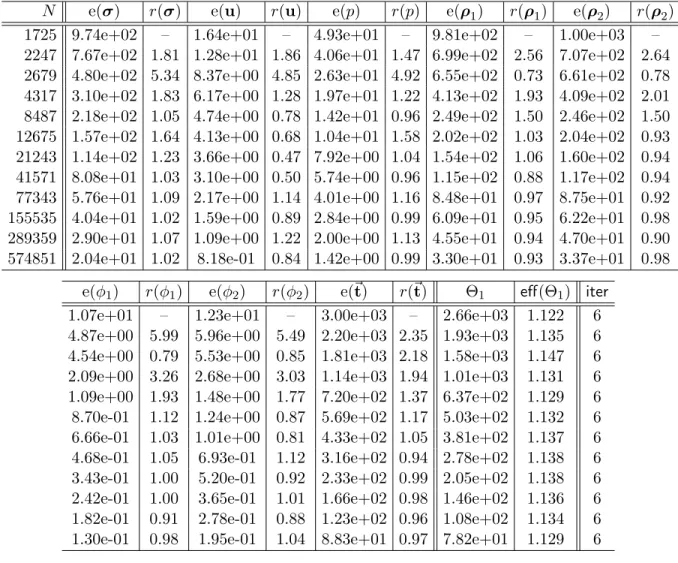
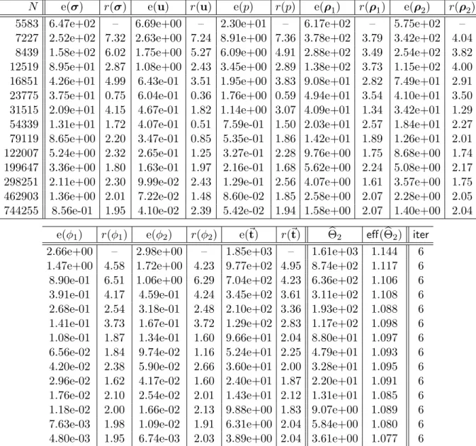
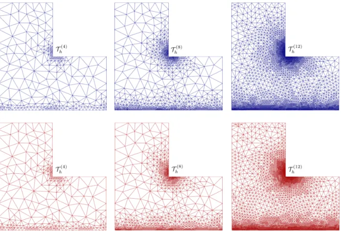
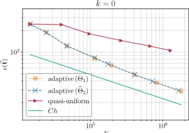
More precisely, in each case we derive a global quantity Θ that is expressed in terms of calculable local indicators Θ_T defined on each element T of a given triangulation T. This information can be afterwards used to localize sources of error and construct an algorithm to efficiently adapt the mesh.

In this way, the estimator Θ is said to be efficient (resp. reliable) if there exists a positive constant C_eff (resp. C_rel), independent of the meshsizes, such that

C_effΘ + h.o.t. ≤ kerrork ≤ C_relΘ + h.o.t. ,

where h.o.t. is a generic expression denoting one or several terms of higher order. We observe that, up to our knowledge, the present work provides the firsta posteriorierror analyses of mixed finite element methods for the coupling of the stationary Brinkman–Forchheimer and double-diffusion equations.

This paper is organized as follows. The remainder of this section introduces some standard notations and functional spaces. In Section 2 we recall from [8] the model problem and its continuous and discrete augmented fully-mixed variational formulations. Next, in Section 3 we provide some preliminary results to be employed in the derivation and analysis of our a posteriori error estimator. The core of the present work is given by Section 4, where we develop the a posteriori error analysis. In Section 4.1 we employ the uniform ellipticity and inf-sup condition of the bilinear forms involved, suitable Helmholtz decompositions in Hilbert and Banach frameworks, the local approximation properties of the Cl´ement and Raviart–Thomas operators, and known estimates from [4] and [26], to derive a reliable residual-based a posteriori error estimator. Then, inverse inequalities, and the localization technique based on element-bubble and edge-bubble functions are utilized in Section 4.2 to prove the efficiency of the estimator. A second (also reliable and efficient) residual-based a posteriori error estimator is introduced and studied in Section 5, where the Helmholtz decomposition in a Hilbert framework is not employed in the corresponding proof of reliability. Finally, numerical results confirming the reliability and efficiency of thea posteriorierror estimators, and showing the good performance of the associated adaptive algorithms, are presented in Section 6.

1.1 Preliminary notations

Let Ω ⊂R^d, d∈ {2,3}, denote a bounded domain with polyhedral boundary Γ, and denote by n the outward unit normal vector on Γ. Standard notation will be adopted for Lebesgue spaces L^p(Ω) and Sobolev spaces W^s,p(Ω), with s ∈ R and p > 1, whose corresponding norms, either for the scalar, vector, or tensor case, are denoted by k · k_0,p;Ω and k · k_s,p;Ω, respectively. In particular, when p= 2, W^s,2(Ω) is also denoted by H^s(Ω), and the writing of its norm and seminorm are simplified tok · k_s,Ω and| · |_s,Ω, respectively. ByMandMwe will denote the corresponding vector and tensor counterparts of the generic scalar functional space M, andk · k, with no subscripts, will stand for the natural norm of either an element or an operator in any product functional space. In turn, for any vector field v = (v_i)_i=1,d, we let ∇v and div(v) be its gradient and divergence, respectively. Furthermore, given tensor fields τ = (τij)i,j=1,d and ζ = (ζij)i,j=1,d, we let div(τ) be the divergence operator div acting along the rows ofτ, and define the transpose, the trace, and the deviatoric tensor of τ, as well as the tensor inner product between τ and ζ, respectively, as

τ^t:= (τji)i,j=1,d, tr(τ) :=

Xd i=1

τii, τ^d:=τ− 1

dtr(τ)I, and τ :ζ :=

Xd i,j=1

τijζij,

where Iis the identity matrix in R^d×d. In what follows, when no confusion arises, | · |will denote the Euclidean norm in R^d or R^d×d. Additionally, given p > 1, we define the following tensor and vector

functional spaces (see [8, Section 2.2] for details):

H0(div; Ω) := n

τ ∈H(div; Ω) : Z

Ω

tr(τ) = 0o

(1.1) and

H(divp; Ω) := n

η∈L²(Ω) : div(η)∈L^p(Ω)o

, (1.2)

endowed with the norms

kτk²_div;Ω := kτk²_0,Ω+kdiv(τ)k²_0,Ω and kηk_divp;Ω := kηk_0,Ω+kdiv(η)k_0,p;Ω,

respectively. In addition, H^1/2(Γ) is the space of traces of functions of H¹(Ω) and H^−1/2(Γ) denotes its dual. Also, by h·,·i_Γ we will denote the corresponding product of duality between H^−1/2(Γ) (resp.

H^−1/2(Γ)) and H^1/2(Γ) (resp. H^1/2(Γ)).

2 The model problem and its variational formulation

In this section we recall from [8] the model problem of interest, its fully-mixed variational formulation, the associated Galerkin scheme, and the main results concerning the corresponding solvability analyses.

2.1 The coupling of the Brinkman–Forchheimer and double-diffusion equations In what follows we consider the model introduced in [29] (see also [8]), which is given by a steady double-diffusive convection system in a fluid saturated porous medium. More precisely, we focus on solving the coupling of the incompressible Brinkman–Forchheimer and double-diffusion equations, which reduces to finding a velocity fieldu, a pressure fieldp, a temperature fieldφ1and a concentration field φ₂, the latter two defining a vectorφ:= (φ₁, φ₂), such that

−ν∆u+K⁻¹u+F|u|u+∇p = f(φ) in Ω, div(u) = 0 in Ω,

−div(Q1∇φ₁) +R1u· ∇φ₁ = 0 in Ω,

−div(Q₂∇φ₂) +R2u· ∇φ₂ = 0 in Ω, u=uD, φ1 =φ1,D, and φ2 = φ2,D on Γ,

Z

Ω

p = 0,

(2.1)

with parameters ν :=Daµ/µe and F:=ϑDaR1, whereDa stands for the Darcy number,µethe viscosity, µ the effective viscosity, R₁ the thermal Rayleigh number, R₂ the solute Rayleigh number, and ϑis a real number that can be calculated experimentally. In addition, the Dirichlet boundary data is given by uD∈H^1/2(Γ),φ1,D∈H^1/2(Γ) and φ2,D∈H^1/2(Γ). Owing to the incompressibility of the fluid and the Dirichlet boundary condition for u, the datumu_Dmust satisfy the compatibility condition

Z

Γ

u_D·n = 0. (2.2)

In turn, the external force f is defined by

f(φ) := −(φ₁−φ_1,r)g+ 1

%(φ₂−φ_2,r)g,

with g representing the potential type gravitational acceleration,φ1,r the reference temperature,φ2,r

the reference concentration of a solute, both of them in L⁴(Ω), and%is another parameter experimen- tally valued that can be assumed to be greater than 1 (see [29, Section 2] for details). In turn, the permeability, thermal diffusion and concentration diffusion tensors are denoted, respectively, byK,Q1

and Q₂, all them lying inL^∞(Ω). Moreover,Kand the inverses of Q₁ andQ₂, are uniformly positive definite tensors, which means that there exist positive constants C_K,C_Q1, and C_Q2, such that

v·K(x)v ≥ C_K|v|² and v·Q⁻¹_j (x)v ≥ C_Qj|v|² ∀v∈Rⁿ,∀x∈Ω, j∈ {1,2}. (2.3) Next, in order to derive a fully-mixed formulation for (2.1), in which the Dirichlet boundary condi- tions become natural ones, we now proceed as in [8], and introduce the pseudostress tensor, and the pseudoheat and pseudodiffusive vectors as further unknowns, that is

σ := ν∇u−pI, ρ₁:=Q1∇φ₁−R1φ1u, ρ₂:=Q2∇φ₂−R2φ2u in Ω. (2.4) In this way, applying the trace operator to σ and utilizing the incompressibility condition div(u) = 0 in Ω, one arrives at

p=−1

dtr(σ) in Ω. (2.5)

Hence, replacing (2.5) back into the first equation of (2.4), we find that our model problem (2.1) can be rewritten, equivalently, as follows: Find (σ,u) and (ρ_j, φ_j), j ∈ {1,2}, in suitable spaces to be indicated below, such that

1

ν σ^d = ∇u in Ω,

−div(σ) +K⁻¹u+F|u|u = f(φ) in Ω, Q⁻¹_j ρ_j+R_jQ⁻¹_j φ_ju = ∇φ_j in Ω,

−div(ρ_j) = 0 in Ω, u=uD and φ = φ_D on Γ,

Z

Ω

tr(σ) = 0,

(2.6)

where the Dirichlet datum for φ is certainly given by φ_D := (φ1,D, φ2,D). At this point we stress that, as suggested by (2.5), pis eliminated from the present formulation and computed afterwards in terms of σ by using that identity. This fact justifies the last equation in (2.6), which ensures that the resulting psatisfies R

Ωp= 0.

2.2 The fully-mixed variational formulation

We begin by recalling from [8, Section 2.2] the augmented fully-mixed variational formulation for the coupling of the Brinkman–Forchheimer and double-diffusion equations (cf. (2.6)), which reads: Find (σ,u)∈H0(div; Ω)×H¹(Ω) and (ρ_j, φj)∈H(div_4/3; Ω)×L⁴(Ω),j ∈ {1,2}, such that

A((σ,u),(τ,v)) +B_u((σ,u),(τ,v)) = F_D(τ,v) +F_φ(τ,v), aj(ρ_j,η_j) +b(η_j, φj) +cj(u;φj,η_j) = Gj(η_j),

b(ρ_j, ψ_j) = 0,

(2.7)

for all (τ,v)∈H0(div; Ω)×H¹(Ω) and for all (η_j, ψj)∈H(div_4/3; Ω)×L⁴(Ω), where, givenw∈H¹(Ω), A, B_w, a_j, b, andc_j(w;·,·) are the forms defined, respectively, as

A((σ,u),(τ,v)) := 1 ν

Z

Ω

σ^d :τ^d+ Z

Ω

Kdiv(σ)·div(τ) +κ₁ Z

Ω

∇u−1 νσ^d

:∇v+κ₂ Z

Γ

u·v, (2.8) B_w((σ,u),(τ,v)) := −F

Z

Ω

K|w|u·div(τ), (2.9) and

a_j(ρ_j,η_j) :=

Z

Ω

Q⁻¹_j ρ_j·η_j, b(η_j, ψ_j) :=

Z

Ω

ψ_jdiv(η_j), (2.10) cj(w;ψj,η_j) := Rj

Z

Ω

Q⁻¹_j ψjw·η_j, (2.11)

for all (σ,u),(τ,v) ∈ H0(div; Ω)×H¹(Ω) and for all (ρ_j, φ_j),(η_j, ψ_j) ∈ H(div_4/3; Ω)×L⁴(Ω). In turn, given ϕ:= (ϕ1, ϕ2)∈L⁴(Ω),FD, Fϕ, and Gj are the bounded linear functionals defined by

FD(τ,v) := hτn,uDi_Γ+κ2

Z

Γ

uD·v, Fϕ(τ,v) := − Z

Ω

K f(ϕ)·div(τ), (2.12) for all (τ,v)∈H0(div; Ω)×H¹(Ω) and

Gj(η_j) :=

η_j·n, φj,D

Γ, (2.13)

for all η_j ∈H(div_4/3; Ω). Notice thatκ₁ andκ₂ are positive parameters that can be taken as (see [8, Lemma 3.2 and eq. (3.36)] for details):

κ1=ν and κ2 = ν

2. (2.14)

These particular values will be used later on for the computational implementation of the Galerkin scheme associated with (2.7). Next, we recall from [8] that u ∈ Wr :=

w∈H¹(Ω) : kwk_1,Ω≤r , where r∈(0, r₀), withr₀:= min{r₁, r₂} and

r₁ := α_A

2FkKk∞ki₄k², r₂:= min{r₂¹, r₂²}, r₂^j := γ_j

2RjkQ⁻¹_j k_∞ki₄k, (2.15) where i4 is the injection ofH¹(Ω) into L⁴(Ω), whereas α_A and γj are positive constants establishing ellipticity and a global inf-sup condition, respectively, of A and the bilinear form A_j that arises after adding the left hand sides of the last two equations of (2.7), but excludingcj (cf. [8, eqns. (3.23) and (3.28)]). According to [8, eq. (3.25)], and using the fact that u∈Wr, we have that the bilinear form A+B_u is uniformly elliptic onHBF:=H0(div; Ω)×H¹(Ω) with positive constantα_A/2 independent of h. This implies that

sup

06=(τ,v)∈H^BF

(A+Bu)((ζ,z),(τ,v))

k(τ,v)k ≥ α_A

2 k(ζ,z)k, (2.16)

for all (ζ,z)∈HBF. In turn, we recall from [8, eq. (3.33)] the following inf-sup condition sup

06=(η_j,ψj)∈HD

a_j(χ_j,η_j) +b(η_j, ϕ_j) +b(χ_j, ψ_j) +c_j(u;ϕ_j,η_j) k(η_j, ψj)k ≥ γ_j

2 k(χ_j, ϕj)k, (2.17)

for all (χ_j, ϕj) ∈ HD := H(div_4/3; Ω)×L⁴(Ω). Further details yielding the solvability of (2.7) were developed in [8, Theorem 3.9]. In particular, we recall for later use the following a prioriestimates

k(σ,u)k ≤ cT

n

ku_Dk_0,Γ+ku_Dk_1/2,Γ+kgk_0,4;Ω kφ_Dk_1/2,Γ+kφ_rk_0,4;Ωo

(2.18)

and X2

j=1

k(ρ_j, φ_j)k ≤ c

eSkφ_Dk_1/2,Γ, (2.19)

where c_T := c_S max

1, cSe , and c_S and c

Se are positive constants defined in [8, eqns. (3.21) and (3.29)].

2.3 The fully-mixed finite element method

We denote byT_h a regular partition of Ω made up of trianglesT (whend= 2) or tetrahedralT (when d= 3) of diameter h_T, and meshsize h := max

h_T : T ∈ T_h . In addition, for each T ∈ T_h, we let RTk(T) be the local Raviart–Thomas space of orderk≥0, i.e.,

RT_k(T) := P_k(T)⊕P_k(T)x,

where P_k(T) is the space of polynomials defined on T of degree ≤ k, P_k(T) stands for its vector version (as indicated in Section 1.1), and x:= (x1, . . . , xd)^t is a generic vector of R^d. Next, we recall from [8, Section 4.3] the finite element spaces

H^σ_h := n

τ_h∈H0(div; Ω) : c^tτ_h|_T ∈RT_k(T) ∀c∈R^d, ∀T ∈ T_ho , H^u_h := n

v_h ∈C(Ω) : v_h|_T ∈P_k+1(T) ∀T ∈ T_ho , H^ρ_h := n

η_h ∈H(div_4/3; Ω) : η_h|_T ∈RT_k(T) ∀T ∈ T_ho , H^φ_h := n

ψ_h∈L⁴(Ω) : ψ_h|_T ∈Pk(T) ∀T ∈ T_ho ,

(2.20)

and set φ_h := (φ_1,h, φ_2,h) ∈H^φ_h := H^φ_h×H^φ_h. Then the Galerkin scheme associated with (2.7) reads:

Find (σ_h,u_h)∈H^σ_h ×H^u_h and (ρ_j,h, φ_j,h)∈H^ρ_h×H^φ_h,j∈ {1,2}, such that

A((σ_h,u_h),(τ_h,v_h)) +Bu_h((σ_h,u_h),(τ_h,v_h)) = F_D(τ_h,v_h) +F_φh(τ_h,v_h), a_j(ρ_j,h,η_j,h) +b(η_j,h, φ_j,h) +c_j(u_h;φ_j,h,η_j,h) = G_j(η_j,h),

b(ρ_j,h, ψ_j,h) = 0,

(2.21)

for all (τ_h,v_h) ∈ H^σ_h ×H^u_h and (η_j,h, ψ_j,h) ∈ H^ρ_h ×H^φ_h. The solvability analysis and a priori error bounds for (2.21) are established in [8, Theorems 4.7, 5.4 and 5.6]. In particular, we recall thea priori estimates

k(σ_h,u_h)k ≤ c_Th n

ku_Dk_0,Γ+ku_Dk_1/2,Γ+kgk_0,4;Ω kφ_Dk_1/2,Γ+kφ_rk_0,4;Ωo

(2.22)

and X2

j=1

k(ρ_j,h, φj,h)k ≤ c

Sehkφ_Dk_1/2,Γ, (2.23)

where c_Th := c_S max

1, cSe_h and c

Se_h is a positive constant, independent of h, defined in [8, eq.

(4.15)].

3 Preliminaries for the a posteriori error analysis

We start by introducing a few useful notations for describing local information on elements and edges or faces depending on wether d= 2 ord= 3, respectively. Let E_h be the set of edges or faces of T_h, whose corresponding diameters are denoted byh_e, and define

E_h(Ω) :=

e∈ E_h : e⊆Ω and E_h(Γ) :=

e∈ E_h : e⊆Γ . For each T ∈ T_h,we let E_h,T be the set of edges or faces of T, and denote

E_h,T(Ω) =

e⊆∂T : e∈ E_h(Ω) and E_h,T(Γ) =

e⊆∂T : e∈ E_h(Γ) . We also define the unit normal vector ne on each edge or face by

ne := (n1, . . . , nd)^t ∀e∈ E_h. Hence, when d= 2 we can define the tangential vector se by

se := (−n2, n1)^t ∀e∈ E_h.

However, when no confusion arises, we will simply write n and s instead ofne and se, respectively.

The usual jump operator [[·]] across internal edges or faces is defined for piecewise continuous matrix, vector, or scalar-valued functions ζ, by

[[ζ]] = (ζ

T+)

e − (ζ

T−)

e with e = ∂T₊∩∂T−,

where T₊ and T− are the elements ofT_h having e as a common edge or face. Finally, for sufficiently smooth scalar ψ, vectorv:= (v₁, . . . , v_d)^t, and tensor fieldsτ := (τ_ij)_i,j=1,d, we let

curl(ψ) :=

− ∂ψ

∂x₂ , ∂ψ

∂x₁ t

, curl(v) :=

curl(v1)^t curl(v₂)^t

ford= 2,

curl(v) :=





∂v2

∂x₁ − ∂v1

∂x₂ , ford= 2,

∇ ×v , ford= 3,

curl(τ) =















curl(τ1) curl(τ₂)

, ford= 2,





curl(τ₁) curl(τ2) curl(τ₃)



 , ford= 3,

γ_∗(v) =





v·s , ford= 2, v×n , ford= 3,

and γ_∗(τ) =











τs , ford= 2,



τ1×n τ2×n τ₃×n



 , ford= 3, where τi is the i-th row of τ and the derivatives involved are taken in the distributional sense.

Now, let Π^k_h :H¹(Ω) → H^ρ_h (cf. (2.20)) be the Raviart–Thomas interpolation operator, which is characterized by the following identities

Z

e

(Π^k_h(v)·n)q = Z

e

(v·n)q ∀edge/facee∈ E_h, ∀q ∈P_k(e) whenk≥0, (3.1)

and Z

T

Π^k_h(v)·q = Z

T

v·q ∀T ∈ T_h, ∀q∈Pk−1(K) when k≥1, (3.2)

for all v∈H¹(Ω). As a consequence of (3.1) and (3.2), it is easy to show that (see [20, Lemma 3.7]) div(Π^k_h(v)) =P_h^k(div(v)),

where P_h^k is the L²(Ω)-orthogonal projector onto the picewise polynomials of degree ≤ k on Ω. A tensor version of Π^k_h, say Π^k_h : H¹(Ω) → H^σ_h, which is defined row-wise by Π^k_h, and a vector version of P_h^k, say P^k_h, which is the L²(Ω)-orthogonal projector onto the piecewise polynomial vectors of degree ≤k, might also be required. The local approximation properties of Π^k_h (and hence of Π^k_h) are established in what follows. For the corresponding proofs we refer to [20, Lemma 3.16] and [4, Lemma 4.2] (see also [3]).

Lemma 3.1 Let p >1. Then, there exist positive constantsc₁,c₂, independent of h, such that for all v∈H¹(Ω) there hold

kv−Π^k_h(v)k0,T ≤ c1hT kvk_1,T ∀T ∈ T_h, and

kv·n−Π^k_h(v)·nk_0,p;e ≤ c₂h^1−1/p_e kvk_1,p;Te ∀e∈ E_h, where T_e is a triangle of T_h containing the edge eon its boundary.

In turn, letI_h: H¹(Ω)→H¹_h(Ω) be the Cl´ement interpolation operator, where H¹_h(Ω) :=n

v∈ C(Ω) : v|_T ∈P₁(T) ∀T ∈ T_ho .

The local approximation properties of this operator are established in the following lemma (see [12]).

Lemma 3.2 There exist positive constants c₃,c₄, independent of h, such that for allv ∈H¹(Ω)there holds

kv−I_h(v)k0,T ≤ c3hT kvk_1,∆(T) ∀T ∈ T_h, and

kv−I_h(v)k_0,e ≤ c₄h^1/2_e kvk_1,∆(e) ∀e∈ E_h, where

∆(T) :=∪n

T⁰ ∈ T_h : T⁰∩T 6=∅o

and ∆(e) :=∪n

T⁰ ∈ T_h: T⁰∩e6=∅o .

In what follows, a vector version of I_h, say I_h :H¹(Ω)→H¹_h(Ω), which is defined component-wise by Ih, will be needed as well. For the forthcoming analysis we will also utilize a couple of results providing stable Helmholtz decompositions for H0(div; Ω) and H(divp; Ω) (cf. (1.1), (1.2)). More precisely, we have the following lemmas.

Lemma 3.3 For each τ ∈H(div; Ω) there exist

a) z∈H²(Ω) and χ∈H¹(Ω) such thatτ =∇z+curl(χ) when d= 2, b) z∈H²(Ω) and χ∈H¹(Ω) such thatτ =∇z+curl(χ) when d= 3.

In addition, in both cases,

kzk_2;Ω+kχk_1,Ω ≤ C_Helkτk_div;Ω,

where C_Hel is a positive constant independent of all the foregoing variables.

Proof. For the proof ofa) andb) we refer to [28, Lemma 3.7] and [21, Theorem 3.1], respectively. We

omit further details.

Lemma 3.4 Let 1< p≤2 when d= 2 and 6/5≤p≤2 when d= 3. Then, for eachη∈H(divp; Ω) there exist

a) ξ ∈W^1,p(Ω)and w∈H¹(Ω)such that η=ξ+ curl(w) when d= 2, b) ξ ∈W^1,p(Ω)and w∈H¹(Ω)such that η=ξ+ curl(w) whend= 3.

In addition, we have that

kξk_1,p;Ω+kwk_1,Ω ≤ C_Helkηk_divp;Ω and kξk_1,p;Ω+kwk_1,Ω ≤ C_Helkηk_divp;Ω,

for d= 2 and d= 3, respectively, where C_Hel is a positive constant independent of all the foregoing variables.

Proof. See [4, Lemma 4.4].

4 First residual-based a posteriori error estimator

In this section we derive a reliable and efficient residual based a posteriori error estimator for the Galerkin scheme (2.21). To this end, in what follows we assume the hypotheses from [8, Theorems 3.9 and 4.7], which guarantee the existence of unique solutions (σ,u,ρ_j, φj) ∈H0(div; Ω)×H¹(Ω)× H(div_4/3; Ω)×L⁴(Ω) and (σh,uh,ρ_j,h, φj,h) ∈H^σ_h ×H^u_h×H^ρ_h×H^φ_h,j∈ {1,2}of the continuous and discrete problems (2.7) and (2.21), respectively. Then, the first global a posteriori error estimator is defined by:

Θ₁ :=



 X

T∈Th

Θ²_BF,T + X2 j=1

Θ²_D,j,T

!



1/2

+



 X

T∈Th

X2 j=1

kdiv(ρ_j,h)k^4/3_0,4/3;T





3/4

, (4.1)

where, for each T ∈ T_h, the local error indicators Θ²_BF,T and Θ²_D,j,T are defined as follows:

Θ²_BF,T := f(φ_h) +div(σ_h)−K⁻¹u_h−F|u_h|u_h²

0,T + ∇u_h− 1 ν σ^d_h

²

0,T

+h²_T curl

1 ν σ^d_h

2

0,T

+ X

e∈E_h,T(Ω)

h_e

γ_∗

1

ν σ^d_h

2

0,e

+ X

e∈E_h,T(Γ)

ku_D−u_hk²_0,e + X

e∈E_h,T(Γ)

he

γ_∗

1

νσ^d_h− ∇u_D

2

0,e

(4.2)

and

Θ²_D,j,T :=h^2−d/2_T

∇φ_j,h−Q⁻¹_j ρ_j,h+Rjφ_j,hu_h²

0,T +h²_T curl

Q⁻¹_j ρ_j,h+Rjφ_j,hu_h²

0,T

+ X

e∈E_h,T(Ω)

h_e hh

γ_∗

Q⁻¹_j ρ_j,h+Rjφ_j,hu_hii²

0,e + X

e∈E_h,T(Γ)

h^1/2_e kφ_j,D−φ_j,hk²_0,4;e

+ X

e∈E_h,T(Γ)

h_e γ_∗

Q⁻¹_j ρ_j,h+Rjφ_j,hu_h

− ∇φ_j,D²

0,e .

(4.3)

Notice that the last term of Θ²_BF,T requires γ_∗(∇uD)

e ∈ L²(e) for all e∈ E_h(Γ), which is overcome below (cf. Lemma 4.4) by simply assuming that u_D∈H¹(Γ). Similarly, the last two terms of Θ²_D,j,T are well defined if we assume that φ_j,D∈H¹(Γ)∩L⁴(Γ) for eachj∈ {1,2}.

The main goal of the present section is to establish, under suitable assumptions, the existence of positive constants C_eff and C_rel, independent of the meshsizes and the continuous and discrete solutions, such that

CeffΘ1+ h.o.t. ≤ k(σ,u)−(σh,uh)k+ X2 j=1

k(ρ_j, φj)−(ρ_j,h, φj,h)k ≤ CrelΘ1, (4.4) where h.o.t. is a generic expression denoting one or several terms of higher order. The upper and lower bounds in (4.4), which are known as the reliability and efficiency of Θ1, are derived below in Sections 4.1 and 4.2, respectively.

4.1 Reliability of the a posteriori error estimator The main result of this section is stated in the following theorem.

Theorem 4.1 Assume that the data uD,φ_D and φ_r satisfy cT_h

r₀ n

ku_Dk_0,Γ+ku_Dk_1/2,Γ+kgk_0,4;Ω 2kφ_Dk_1/2,Γ+kφ_rk_0,4;Ωo

≤ 1

2, (4.5)

with r0 := min{r1, r2}, and r1, r2 are defined in (2.15). Then, there exists a positive constant Crel, independent of h, such that

k(σ,u)−(σh,uh)k+ X2 j=1

k(ρ_j, φj)−(ρ_j,h, φj,h)k ≤ CrelΘ1. (4.6) We begin the derivation of (4.6) with a preliminary lemma, for which we first recall that

HBF:=H0(div; Ω)×H¹(Ω) and H_D :=H(div_4/3; Ω)×L⁴(Ω).

Lemma 4.2 Assume that the datauD,φ_Dandφ_r satisfy (4.5). Then, there exists a positive constant C, independent of h, such that

k(σ,u)−(σ_h,u_h)k+ X2 j=1

k(ρ_j, φj)−(ρ_j,h, φ_j,h)k

≤ C sup

06=(τ,v)∈H^BF

|R^BF(τ,v)|

k(τ,v)k + X2 j=1

sup

06=(η_j,ψj)∈HD

|R^D_j(η_j, ψj)|

k(η_j, ψ_j)k

! ,

(4.7)

where R^BF:HBF→R and R^D_j :HD →R are the residual functionals given by

R^BF(τ,v) =F_D(τ,v) +F_φh(τ,v)−A((σ_h,u_h),(τ,v))−B_uh((σ_h,u_h),(τ,v)) for all (τ,v)∈HBF, and

R^D_j(η_j, ψj) =Gj(η_j)−aj(ρ_j,h,η_j)−b(η_j, φj,h)−b(ρ_j,h, ψj)−cj(uh;φj,h,η_j) for all (η_j, ψ_j)∈H_D.

Proof. First, applying the inf-sup condition (2.16) to the error (ζ,z) = (σ−σh,u−uh), adding and substractingB_uh((σ_h,u_h),(τ,v)) andF_φh(τ,v), and using the first equation of (2.7), we deduce that

αA

2 k(σ−σ_h,u−u_h)k ≤ sup

06=(τ,v)∈H^BF

R^BF(τ,v) k(τ,v)k

+ sup

06=(τ,v)∈H^BF

B_u−uh((σ_h,u_h),(τ,v))

k(τ,v)k + sup

06=(τ,v)∈H^BF

F_φ−φ

h(τ,v) k(τ,v)k .

(4.8)

In turn, the continuities of B_w (cf. (2.9)) and F_ϕ (cf. (2.12)) establish (cf. [8, eqns. (3.4), (3.9)]) Bu−u_h((σh,uh),(τ,v))≤FkKk∞ki₄k²ku_hk_1,Ωku−uhk_1,Ωkτk_div;Ω,

F_φ−φ

h(τ,v)≤ kKk_∞kgk_0,4;Ωkφ−φ_hk_0,4;Ωkτk_div;Ω, which, replaced back into (4.8), yields

k(σ−σ_h,u−u_h)k

≤ 2

α_A sup

06=(τ,v)∈HBF

R^BF(τ,v) k(τ,v)k + 1

r₁ku_hk_1,Ωku−u_hk_1,Ω+C_Skgk_0,4;Ωkφ−φ_hk_0,4;Ω,

(4.9)

whereC_S := 2kKk_∞/α_A(cf. [8, eq. (3.40)]) andr₁is defined in (2.15). Similarly, applying the inf-sup condition (2.17) to (χ_j, ϕj) = (ρ_j −ρ_j,h, φj−φj,h), making use of the second and third equations of (2.7), adding and substracting cj(u_h;φ_j,h,η_j), and using the continuity of cj, which states that (cf.

[8, eq. (3.7)]) cj(w;ψ,η) ≤ RjkQ⁻¹_j k ki₄k kwk_1,Ωkψk_0,4;Ωkηk_div4/3;Ω, we deduce that

γ_j

2 k(ρ_j−ρ_j,h, φj−φj,h)k ≤ sup

06=(η_j,ψj)∈HD

R^D_j(η_j, ψ_j)

k(η_j, ψj)k + sup

06=(η_j,ψj)∈HD

c_j(u−u_h;φ_j,h,η_j) kη_jk_div4/3;Ω

≤ sup

06=(η_j,ψj)∈HD

R^D_j(η_j, ψj)

k(η_j, ψ_j)k +R_jkQ⁻¹_j k ki₄k kφ_j,hk_0,4;Ωku−u_hk_1,Ω.

Thus, summing up over j ∈ {1,2}, recalling the definition of r2 in (2.15) and using (2.23) to bound kφ_hk_0,4;Ω :=kφ_1,hk_0,4;Ω+kφ_2,hk_0,4;Ω, we obtain

X2 j=1

k(ρ_j −ρ_j,h, φ_j−φ_j,h)k ≤ X2 j=1

2

γ_j sup

06=(η_j,ψj)∈HD

R^D_j(η_j, ψj) k(η_j, ψ_j)k +c_eS

h

r₂ kφ_Dk_1/2,Γku−u_hk_1,Ω, (4.10) withc

eSh >0 defined in [8, eq. (4.15)]. Then, using the estimate (4.10) to bound the last term in (4.9), recalling the definition of r₀ in (2.15), using (2.22) to bound ku_hk_1,Ω, and recalling thatC_S and c

eSh, as well as 1/r₁ and 1/r₂, are bounded by c_Th and 1/r₀ (cf. [8, eq. (3.43)]), respectively, we deduce that

k(σ−σh,u−uh)k

≤ C1 sup

06=(τ,v)∈HBF

|R^BF(τ,v)|

k(τ,v)k + C2

X2 j=1

sup

06=(η_j,ψj)∈HD

|R^D_j(η_j, ψ_j)|

k(η_j, ψj)k +cT_h

r₀ n

ku_Dk_0,Γ+ku_Dk_1/2,Γ+kgk_0,4;Ω 2kφ_Dk_1/2,Γ+kφ_rk_0,4;Ωo

ku−uhk_1,Ω,

(4.11)

with C1, C2 >0, independent of h. Thus, according to the assumption (4.5), (4.11) yields k(σ−σh,u−uh)k ≤ Cb1 sup

06=(τ,v)∈HBF

|R^BF(τ,v)|

k(τ,v)k + Cb2

X2 j=1

sup

06=(η_j,ψj)∈HD

|R^D_j(η_j, ψ_j)|

k(η_j, ψj)k , (4.12) withCb₁,Cb₂ >0, independent ofh. Next, using (4.12) to bound the last term in (4.10), we easily find that

X2 j=1

k(ρ_j −ρ_j,h, φ_j−φ_j,h)k ≤ Cb₃ sup

06=(τ,v)∈H^BF

|R^BF(τ,v)|

k(τ,v)k + Cb₄ X2 j=1

sup

06=(η_j,ψj)∈HD

|R^D_j(η_j, ψj)|

k(η_j, ψ_j)k , (4.13) with Cb3,Cb4 >0, independent of h. In this way, estimate (4.7) follows from (4.12) and (4.13).

We now aim to bound the suprema in (4.7). Indeed, in virtue of the definitions of the forms A, Bw, aj, b and cj (cf. (2.8)–(2.11)), we find that, for any (τ,v) ∈ H0(div; Ω) ×H¹(Ω) and (η_j, ψj)∈H(div_4/3; Ω)×L⁴(Ω),j ∈ {1,2}, there holds

R^BF(τ,v) =R^BF₁ (τ) +R^BF₂ (v) and R^D_j(η_j, ψ_j) =R^D_j,1(η_j) +R^D_j,2(ψ_j), where

R^BF₁ (τ) = hτn,uDi_Γ− 1 ν

Z

Ω

σ^d_h:τ^d− Z

Ω

u_h·div(τ)

− Z

Ω

K f(φ_h) +div(σ_h)−K⁻¹u_h−F|u_h|u_h

·div(τ),

(4.14)

R^BF₂ (v) = κ2

Z

Γ

(uD−uh)·v−κ1

Z

Ω

∇u_h−1 νσ^d_h

:∇v, (4.15)

R^D_j,1(η_j) =

η_j·n, φ_j,D

Γ− Z

Ω

Q⁻¹_j ρ_j,h+Rjφ_j,hu_h

·η_j − Z

Ω

φ_j,hdiv(η_j), (4.16) and

R^D_j,2(ψ_j) = − Z

Ω

ψ_jdiv(ρ_j,h). (4.17)

Notice that for convenience of the subsequent analysis we have added and subtracted the term given by R

Ωu_h·div(τ) in (4.14). Then, the supremum in (4.7) can be bounded in terms of R^BF₁ ,R^BF₂ ,R^D_j,1, and R^D_j,2 as follows

k(σ,u)−(σ_h,u_h)k+ X2 j=1

k(ρ_j, φj)−(ρ_j,h, φ_j,h)k

≤ C n

kR^BF₁ k_H0(div;Ω)⁰ +kR^BF₂ k_H1(Ω)⁰ + X2 j=1

kR^D_j,1k_H(div

4/3;Ω)⁰+kR^D_j,2k_L4(Ω)⁰

o ,

(4.18)

and hence our next purpose is to derive suitable upper bounds for each one of the terms on the right hand side of (4.18). We begin by establishing the corresponding estimates for R^BF₂ and R^D_j,2 (cf.

(4.15) and (4.17)), which follow from a straightforward application of the Cauchy–Schwarz and H¨older inequalities.

Lemma 4.3 There exist positive constants C1, C2, independent of h, such that

kR^BF₂ k_H1(Ω)⁰ ≤ C1



 X

T∈T_h

∇u_h− 1 νσ^d_h

²

0,T + X

e∈E_h,T(Γ)

ku_D−uhk²_0,e

!



1/2

and

X2 j=1

kR^D_j,2k_L4(Ω)⁰ ≤ C₂



 X

T∈Th

X2 j=1

kdiv(ρ_j,h)k^4/3_0,4/3;T





3/4

.

We now bound the termkR^BF₁ k_H0(div;Ω)0. To this end, we first observe that integrating by parts the expression R

Ωuh·div(τ) in (4.14), the functional R^BF₁ can be rewritten as follows R^BF₁ (τ) =hτn,uD−uhi_Γ+

Z

Ω

∇u_h− 1 ν σ^d_h

:τ

− Z

Ω

K f(φ_h) +div(σ_h)−K⁻¹u_h−F|u_h|u_h

·div(τ).

(4.19)

For simplicity, we prove the aforementioned result for the two-dimensional case. The three dimensional one proceeds analogously. Givenτ ∈H0(div; Ω), it follows from Lemma 3.3 that there existz∈H²(Ω) and χ∈H¹(Ω), such that τ =∇z+curl(χ) in Ω, and

kzk_2,Ω+kχk_1,Ω ≤ CHelkτk_div;Ω. (4.20) Then, we set τ_h := Π^k_h(∇z) +curl(Ih(χ)) +c₀I, wherec₀ ∈ R is chosen so that R

Ωtr(τh) = 0. In addition, bearing in mind the definition of R^BF₁ (cf. (4.14)), and employing the first equation of the Galerkin scheme (2.21) and the compatibility condition (2.2), we deduce that R^BF₁ (τ_h) = 0, whence

R^BF₁ (τ) = R^BF₁ (τ−τ_h) = R^BF₁ (∇z−Π^k_h(∇z)) +R^BF₁ (curl(χ−I_h(χ))). (4.21) The following lemma establishes the estimate for R^BF₁ .

Lemma 4.4 Assume that u_D ∈H¹(Γ). Then, there exists a positive constant C, independent of h, such that

kR^BF₁ k_H0(div;Ω)0 ≤ C ( X

T∈T_h

Θ²_BF,T )1/2

, where

Θ²_BF,T := f(φ_h) +div(σ_h)−K⁻¹u_h−F|u_h|u_h²

0,T + h²_T

∇u_h− 1 ν σ^d_h

²_0,T +h²_T

curl

1 ν σ^d_h

2

0,T

+ X

e∈E_h,T(Ω)

he

γ_∗

1

ν σ^d_h

2

0,e

+ X

e∈E_h,T(Γ)

he

γ_∗

1

ν σ^d_h− ∇u_D

2

0,e

+ X

e∈E_h,T(Γ)

heku_D−u_hk²_0,e.

(4.22)