Tracking the Best Quantizer

(1)

Tracking the Best Quantizer

András György Tamás Linder Gábor Lugosi IEEE Transactions on Information Theory

Submitted: September 15, 2006

Abstract

An algorithm is presented for online prediction that allows to track the best expert efficiently even when the number of experts is exponentially large, provided that the set of experts has a certain additive structure. As an example we work out the case where each expert is represented by a path in a directed graph and the loss of each expert is the sum of the weights over the edges in the path. These results are then used to construct universal limited-delay schemes for lossy coding of individual sequences. In particular, we consider the problem of tracking the best scalar quantizer that is adaptively matched to the source sequence with piecewise different behavior. A randomized algorithm is presented which can perform, on any source sequence, asymptotically as well as the best scalar quantization algorithm that is matched to the sequence and is allowed to change the employed quantizer for a given number of times. The complexity of the algorithm is quadratic in the sequence length, but at the price of some deterioration in performance, the complexity can be made linear. Analogous results are obtained for sequential multiresolution and multiple description scalar quantization of individual sequences.

Index Terms: Algorithmic efficiency, individual sequences, lossy source coding, multiple description quantization, multiresolution coding, non-stationary sources, sequential prediction, sequential coding, scalar quantization.

A. Gy¨orgy is with the Machine Learning Research Group, Computer and Automation Research In- stitute of the Hungarian Academy of Sciences, Kende u. 13-17, Budapest, Hungary, H-1111 (email:

[email protected]). T. Linder is with the Department of Mathematics and Statistics, Queen’s University, Kingston, Ontario, Canada K7L 3N6 (email: [email protected]). G. Lugosi is with ICREA and the Department of Economics, Pompeu Fabra University, Ramon Trias Fargas 25-27, 08005 Barcelona, Spain (email: [email protected]).

This research was supported in part by the Natural Sciences and Engineering Research Council (NSERC) of Canada, the NATO Science Fellowship of Canada, the J´anos Bolyai Research Scholarship of the Hungarian Academy of Sciences, the Mobile Innovation Center of Hungary, Spanish Ministry of Science and Technology and FEDER, grant BMF2003-03324, and by the PASCAL Network of Excellence under EC grant no. 506778.

(2)

1 Introduction

In this paper we consider limited-delay lossy coding schemes for individual sequences.

Our goal is to provide a universal coding method which can dynamically adapt to the changes in the source behavior, with particular emphasis on the situation where the source’s behavior can change a given number of times (which is a function of the sequence length). We concentrate on low-complexity methods that perform uniformly well with respect to a given reference coder class on every individual (deterministic) sequence.

In this individual-sequence setting no probabilistic assumptions are made on the source sequence, which provides a natural model for situations where very little is known about the source to be encoded.

Consider the widely used model for fixed-rate lossy source coding at rate R where an infinite sequence of real-valued source symbols x1, x2, . . . is transformed into a sequence of channel symbolsb1, b2, . . .taking values from the finite channel alphabet {1,2, . . . , M}, M = 2^R. These channel symbols are losslessly transmitted and then used to produce the reproduction sequence ˆx1,xˆ2, . . .. The scheme is said to have delay δ if the reproduction symbol ˆxn can be decoded at most δ time instants after xn was available at the encoder.

A general model for this situation is that each channel symbol bn depends only on the source symbols x1, . . . , xn+δ, and the reproduction ˆxn for the source symbol xn depends only on the channel symbolsb1, . . . , bn. Thus, the encoder produces bn as soon asxn+δ is available, and the decoder can produce ˆxn whenbn is received.

The performance of a scheme is measured with respect to a reference class of coding schemes, and the goal is to perform, on any source sequence, asymptotically as well as the best scheme in the reference class. Thus, the performance is measured by the distortion redundancy defined as the maximum, over all source sequences of length n, of the difference of the normalized cumulative distortion of our scheme and the normalized cumulative distortion of the best scheme in the reference class.

In the initial study of zero-delay coding for individual sequences [1], the reference class was the class of all scalar quantizers, and a coding scheme was provided (using com- mon randomization at the encoder and the decoder) whose distortion redundancy was O(n^−1/5logn) for bounded sequences of length n. The results in [1] were improved and generalized by Weissman and Merhav [2] who constructed schemes that can compete with any finite set of limited-delay finite-memory coding schemes without requiring that the decoder have access to the randomization sequence. The resulting scheme has distortion redundancy O(n^−1/3log^2/3N), where N is the size of the reference coder class. To our knowledge, this is the best known redundancy bound for this problem. In the special case where the reference class is the (infinite) set of scalar quantizers, anO(n^−1/3logn) distortion redundancy can be achieved by approximating the reference class by an appropriately

(3)

chosen finite set of quantizers.

The coding schemes of [1] and [2] are based on the theory of prediction using expert advice. The basic theoretical results were established by Hannan [3] and Blackwell [4]

in the 1950’s and brought to the center of attention in learning theory in the 1990’s by Vovk [5], Littlestone and Warmuth [6], Cesa-Bianchi et al. [7]; see also Cesa-Bianchi and Lugosi [8] for a comprehensive treatment. These results show that it is possible to construct algorithms for online prediction that predict an arbitrary sequence of outcomes almost as well as the best ofN experts in the sense that the cumulative loss of the predictor is at most as large as that of the best expert plus a term proportional to p

lnN/n for any bounded loss function, where n is the number of rounds in the prediction game. The logarithmic dependence on the number of experts makes it possible to obtain meaningful bounds even when the pool of experts is very large.

Unfortunately, the basic prediction algorithms, such as the exponentially weighted average predictor, which was applied both in [1] and [2], have computational complexity which is proportional to the number of experts and are therefore infeasible when this number is very large. Thus, although the coding schemes of [1] and [2] have the attractive property of performing uniformly well on individual sequences, they are computationally inefficient. For example, for the reference class of scalar quantizers, these methods use about n^c²^R quantizers as “experts” where c= 1/5 for the scheme in [1] and c = 1/3 for the scheme in [2] andRis the rate of the scheme, resulting in a computational complexity that is polynomial in n with degree that is proportional to M = 2^R. This complexity comes from the fact that, in order to approximate the performance of the best scalar quantizer, these methods have to calculate and store the cumulative distortion of each of the approximately n^c²^R quantizers. Clearly, even for moderate values of the encoding rate, this complexity becomes prohibitive.

For more general finite reference classes, the method of [2] has to maintain a weight for each of the N reference codes. This results in a computational complexity of order nN, which only allows the use of small reference classes. When the reference class is an infinite set of codes, the method is applied to a finite approximation of the reference class, which can result in a prohibitively large N if the approximation is to be close.

Fortunately, in many applications the set of experts has a certain structure that may be exploited in the construction of efficient prediction algorithms. Examples of structured classes of experts for which efficient algorithms have been constructed include prunings of decision trees (Helmbold and Schapire [9], Pereira and Singer [10]), and planar decision graphs (Mohri [11] and Takimoto and Warmuth [12],[13]). These algorithms are all based on efficient implementations of the exponentially weighted average predictor.

Using a similar approach which exploits the special structure of scalar quantizers, in [14]

(4)

we provided an efficient implementation of the algorithm of [2] for the reference class of scalar quantizers. In this algorithm, the encoding complexity is reduced toO(n^4/3) while maintaining the O(n^−1/3logn) distortion redundancy. Moreover, the complexity can be made linear in the sequence length at the price of increasing the distortion redundancy toO(n^−1/4√

logn).

In the prediction context, a different approach was taken by Kalai and Vempala [15]

who considered Hannan’s original predictor [3] and showed that it may be used to obtain efficient algorithms for a large class of problems that they call “geometric experts.” Based on this method, a zero-delay quantization algorithm with linear encoding complexity was given in [16] which is conceptually simpler than the coding method of [14], and has only a slightly larger distortion redundancy O(n^−1/4logn). Recently Matloub and Weissman [17] extended the general coding scheme of [2] and the method of efficient implementation of [16] to zero-delay joint source-channel coding of individual sequences.

As suggested in [2], it is an interesting open problem to find an algorithm of low complexity that is able to approximate the performance of the best scheme from a larger reference class. However, it seems that to date no low-complexity algorithms have been devised which work for more powerful reference classes than the class of scalar quantizers.

In this paper we consider a more general reference class in which each reference scheme partitions the input sequence into contiguous segments and for each segment a different delay-δ code from a finite base reference classF may be employed. If a combined scheme can change the applied codemtimes for an input sequence of lengthn, then the number of such schemes isPm

j=0 n j

|F|(|F| −1)^j. If one has to maintain a weight for each reference code, the implementation is infeasible even for a very small F, as the straightforward implementation requires O((n+m)^m|F|^m) computations. However, as we will show in this paper, the structure of the reference codes provides a possibility to overcome this problem.

In the probabilistic setting, the somewhat related problem of efficient sequential lossless coding of piecewise stationary memoryless sources has been studied by Willems [18], Shamir and Merhav [19] and Shamir and Costello [20], and some of the algorithms we develop in this paper are close in spirit to that of Willems.

The corresponding prediction problem for individual sequences, known as the problem of tracking the best expert, is perhaps the best known example of a structured reference class. In this problem, a small number of “base” experts is given and the goal of the predictor is to predict as well as the best “meta” expert that is formed by certain allowable sequences of base experts. A sequence is allowable if it consists of at most m+ 1 blocks such that in each block the meta expert predicts according to a fixed base expert. If there are N base experts and the length of the prediction game is n, then the total number

(5)

of meta experts is Pm j=0

n j

N(N − 1)^j. For this problem Herbster and Warmuth [21]

exhibited computationally efficient algorithms that predict almost as well as the best of the meta experts and have regret bounds that depend on the logarithm of the number of the (meta) experts. See also Auer and Warmuth [22], Bousquet and Warmuth [23], and Herbster and Warmuth [24] for various extensions and powerful variants of the problem.

However, these methods become computationally too expensive if the “base” reference class is very large.

In this paper we develop efficient algorithms to track the best expert in the case when the class of “base” experts is already very large, but has a certain structure. Thus, in a sense, we consider a combination of the two types of structured experts described above. Our approach is based on a suitable modification of the original tracking algorithm of Herbster and Warmuth [21] that can handle large, structured expert classes. This modification is described in Section 2. In Section 3 we use the modified tracking predictor algorithm combined with the coding method of Weissman and Merhav [2] to obtain codes which can track any finite class of limited-delay finite-memory codes efficiently. The proposed method has computational complexity of order n|F|, significantly less than the O((n+m)^m|F|^m) complexity of the algorithm in [2] when applied to this problem, and has basically the same distortion redundancy. In Section 4 we illustrate our new prediction method on a problem in which a base expert is associated with a path in a directed graph and the loss of a base expert is the sum of the weights over the path (which may change in every round of the prediction game). The special structure of the experts allows efficient implementation of tracking. This graph representation of the experts is used in Section 5 to obtain efficient coding algorithms to track the best scalar quantizer (i.e., to code asymptotically as well as the best combined coding scheme from scalar quantizers). Finally, in Section 6 we consider two network quantization versions of this problem: tracking the best multiple description scalar quantizer and tracking the best multiresolution scalar quantizer (among quantizers with interval cells). The encoding and decoding complexity of each of these algorithms can be made linear in the sequence length at the price of some performance deterioration.

2 Tracking the best expert: a variation

In this section we present a modification of a prediction algorithm by Herbster and War- muth [21] for tracking the best expert. This modification will facilitate efficient implementation if the number of experts is very large.

The online decision problem we consider is described as follows. Suppose we want to use a sequential decision scheme to make predictions concerning the outcomes of a

(6)

sequence y1, y2, . . . taking values in a setY. We assume that the (randomized) predictor has access to a sequence of independent random variables U1, U2, . . . which are uniformly distributed over the interval [0,1]. At each time instantt = 1,2, . . ., the predictor observes Ut, and based on Ut and the past input values y^t−1 = (y1, . . . , yt−1) produces an “action”

ˆ

yt∈Yˆ, where ˆY is the set of predictor actions that may not be the same asY. Then the predictor can observe the next input symbolyt and calculate its loss `(yt,yˆt) with respect to some bounded loss function `:Y ×Y →b [0, B], where B >0.

Formally, the prediction game is defined as follows:

Parameters: number N of base experts, outcome space Y, action space ˆY, loss function `:Y ×Y →ˆ [0, B], numberT of rounds.

For each round t= 1, . . . , T,

(1) each (base) expert forms its prediction ˆy_t⁽ⁱ⁾ ∈Yˆ, i= 1, . . . , N;

(2) the predictor observes the predictions of the base experts and the random variable U_t, and chooses an estimate ˆy_t∈Yˆ;

(3) the environment reveals the next outcomeyt ∈ Y.

The cumulative loss of the sequential scheme at timeT is given by LT =

XT t=1

`(yt,yˆt).

One of the most popular algorithms for the on-line prediction game described above is the exponentially weighted average predictor (see [5], [6], [7]) which is defined as follows:

let η > 0 be a parameter and to each i = 1, . . . , N assign the initial weight w1,i = 1/N.

At time instants t = 1,2, . . . , T, let v⁽ⁱ⁾_t = wt,i/Wt where Wt = PN

i=1wt,i and predict ˆyt

randomly according to the distributionP{yˆt= ˆy⁽ⁱ⁾_t }=v_t⁽ⁱ⁾. After observingyt, update the weights bywt+1,i =wt,ie^−η`(y^t^,ˆ^y^t⁽ⁱ⁾⁾. This yieldsv_t⁽ⁱ⁾ =e^−η^P^t−1^t⁰⁼¹^`(y^t^,ˆ^y⁽ⁱ⁾^t ⁾/PN

j=1e^−η^P^t−1^t⁰⁼¹^`(y^t^,ˆ^y^t⁽ⁱ⁾⁾, that is, v_t⁽ⁱ⁾ is proportional to the “exponential” cumulative performance of expert i up to time t−1. It is well known that the expected cumulative regret of the exponentially weighted average predictor may be bounded, for all possible sequences generated by the environment, by

E LT − min

i=1,...,N

XT t=1

`(yt,yˆ⁽ⁱ⁾_t )

!

≤B

lnN η +nη

8

,

(7)

where the expectation is understood with respect to the randomization sequenceU1, . . . , UT

of the predictor. In particular, ifη=Bp

8 lnN/T is chosen to optimize the upper bound, then the bound becomes Bp

(T /2) lnN. (For various versions and more discussion on the performance of this algorithm, we refer the reader to [8].)

The exponentially weighted average algorithm is thus guaranteed to perform, on the average, almost as well as the expert with the smallest cumulative loss. A more ambitious goal of the predictor is to achieve a cumulative loss (almost) as small as the best tracking of the N base experts. More precisely, to describe the loss the predictor is compared to, consider the following “m-partition” prediction scheme: The sequence of examples y1, . . . , yT is partitioned intom+ 1 contiguous segments, and on each segment the scheme assigns exactly one of the N base experts. Formally, an m-partition P(T, m,t,e) of the first T samples is given by anm-tuplet= (t1, . . . , tm) such thatt0 = 0< t1 <· · ·< tm <

T = tm+1, and an (m+ 1)-vector e = (e0, . . . , em) where ei ∈ {1, . . . , N}. At each time instant t, ti < t≤ti+1, expert ei is used to predict yt. The cumulative loss of a partition P(T, m,t,e) is

L(P(T, m,t,e)) = Xm

i=0 ti+1

X

t=ti+1

`(yt,yˆ_t^(eⁱ⁾) = Xm

i=0

L((ti, ti+1], ei) where for any time interval I, L(I, i) = P

t∈I`(yt,yˆ⁽ⁱ⁾_t ) denotes the cumulative loss of expert i in I. Here and later in the paper we adopt the convention that in case the summation is over an empty index set, the sum is defined to be zero (e.g., for a > b, L([a, b], i) = 0).

The goal of the predictor is to perform nearly as well as the best partition, that is, to keep the normalized regret

1 T

LT −min

t,e L(P(T, m,t,e))

as small as possible (with high probability) for all possible outcome sequences. A slightly different goal is to keep the normalized expected regret

1 TE

LT −min

t,e L(P(T, m,t,e))

as small as possible, where the expectation is taken with respect to the randomizing sequence U^T = (U1, . . . , UT).

Herbster and Warmuth [21] constructed a so-called “fixed-share” share update algorithm for the tracking prediction problem. Below we present a slightly modified version of this algorithm. While this modification was also introduced by Bousquet and Warmuth [23], the performance bounds provided there are insufficient for our purposes.

(8)

Algorithm 1 Fix the positive numbers η and α < 1, and initialize weights w^s_1,i = 1/N fori= 1, . . . , N. At time instantst = 1,2, . . . , T letv⁽ⁱ⁾_t =w_t,i^s /Wt

where Wt=PN

i=1w^s_t,i, and predict yˆt randomly according to the distribution P{yˆt= ˆy⁽ⁱ⁾_t }=v_t⁽ⁱ⁾. (1) After observing yt, for all i= 1, . . . , N, let

w_t,i^m =w^s_t,ie^−η`(y^t^,ˆ^y⁽ⁱ⁾^t ⁾ (2) and

w^s_t+1,i= αWt+1

N + (1−α)w^m_t,i (3)

where Wt+1 =PN i=1w_t,i^m. Observe thatPN

i=1w^s_t+1,i =PN

i=1w_t,i^m =Wt+1; thus there is no ambiguity in the definition ofWt+1. Note that equation (3) is slightly changed compared to the original algorithm of [21].

The following theorem bounds the loss of the algorithm. The proof is quite similar to that in [21] and therefore it is deferred to the appendix.

Theorem 1 For all positive integersm, T withT ≥m+1, real numbers0< α <1, η >0, and 0< p <1, and for any sequence y₁, . . . , y_T and loss function ` :Y ×Y →ˆ [0, B], with probability at least 1−p, the regret of Algorithm 1 can be bounded as

LT −min

t,e L(P(T, m,t,e))

≤ 1 ηln

N^m+1 α^m(1−α)^T^−m−1

+T ηB² 8 +B

rT ln(1/p)

2 (4)

and the expected regret can be bounded as E

LT −min

t,e L(P(T, m,t,e))

≤ 1 η ln

N^m+1 α^m(1−α)^T^−m−1

+ T ηB²

8 . (5)

In particular, if α = _T^m₋₁ <1 and η is chosen to minimize the above bound as

η= vu ut8 ln

N^m+1 α^m(1−α)^T−m−1

T B² (6)

we have

LT −min

t,e L(P(T, m,t,e))

≤ T^1/2 B

√2 r

(m+ 1) lnN+mlnT −1

m +m+B

rTln(1/p)

2 (7)

(9)

and

E

LT −min

t,e L(P(T, m,t,e))

≤ T^1/2 B

√2 r

(m+ 1) lnN +mlnT −1

m +m . (8)

Remark. If the number of experts N is proportional to T^γ for some γ > 0, then the bound in (8) is of order p

(mT) lnT, and so the normalized expected regret is 1

TE

L_T −min

t,e L(P(T, m,t,e))

=Op

(m/T) lnT .

That is, the rate of convergence is the same (up to a constant factor) as if we competed with the best static expert on a segment of average length T /m.

2.1 Implementation of Algorithm 1

If the number of expertsN is large, for example,N =T^γfor some largeγ >1, then the implementation of Algorithm 1 may become computationally prohibitive. The main message of this section is the nontrivial observation that if the standard exponentially weighted prediction algorithm can be efficiently implemented, then one can also efficiently imple- ment Algorithm 1. The main step toward demonstrating this is the following alternative expression for the weights in Algorithm 1.

Lemma 1 For any t= 2, . . . , T, the probability v_t⁽ⁱ⁾ and the corresponding normalization factor Wt in Algorithm 1 can be obtained as

v_t⁽ⁱ⁾ = (1−α)^t−1 N Wt

e−ηL([1,t−1],i)+ α N Wt

Xt−1 t⁰=2

(1−α)^t−t⁰Wt⁰e^−ηL([t⁰^,t−1],i)+ α

N (9)

Wt = α N

Xt−1 t⁰=2

(1−α)^t−1−t⁰Wt⁰Zt⁰,t−1+ (1−α)^t−2

N Z1,t−1 (10)

where Zt⁰,t−1 = PN

i=1e^−ηL([t⁰^,t−1],i) is the sum of the (unnormalized) weights assigned to the experts by the exponentially weighted prediction method for the input samples (yt⁰, . . . , yt−1).

Proof. The expressions in the lemma follow directly from the recursive definition of the weights{w_t,i^s }. First we show that for t= 1, . . . , T,

w_t,i^m = α N

Xt

(1−α)^t−t⁰Wt⁰e^−ηL([t⁰^,t],i)+(1−α)^t−1

N e−ηL([1,t],i) (11)

(10)

w_t+1,i^s = α

NW_t+1+ α N

Xt t⁰=2

(1−α)^t+1−t⁰W_t⁰e^−ηL([t⁰^,t],i)+ (1−α)^t

N e−ηL([1,t],i). (12) Clearly, for a given t, (11) implies (12) by the definition (3). Since w_1,i^s = 1/N for every expert i, (11) and (12) hold for t= 1 and t = 2 (for t= 1 the summations are 0 in both equations). Now assume that they hold for somet≥2. We show that then (11) holds for t+ 1. By definition,

w_t+1,i^m = w^s_t+1,ie^−η`(y^t+1^,ˆ^y⁽ⁱ⁾^t+1⁾

= α

NW_t+1e^−η`(y^t+1^,ˆ^y⁽ⁱ⁾^t+1⁾+ α N

Xt t⁰=2

(1−α)^t+1−t⁰W_t⁰e^−ηL([t⁰^,t+1],i) +(1−α)^t

N e−ηL([1,t+1],i)

= α

N Xt+1 t⁰=2

(1−α)^t+1−t⁰Wt⁰e^−ηL([t⁰^,t+1],i)+(1−α)^t

N e−ηL([1,t+1],i)

thus (11) and (12) hold for all t = 1, . . . , T. Now (9) follows from (12) by normalization for t= 2, . . . , T + 1. Finally, (10) can easily be proved from (11), as for anyt= 2, . . . , T,

Wt = XN

i=1

w_t−1,i^m

= XN

i=1

α N

Xt−1 t⁰=2

(1−α)^t−1−t⁰W_t⁰e^−ηL([t⁰^,t−1],i)+ (1−α)^t−2

N e−ηL([1,t−1],i)

!

= α

N Xt−1 t⁰=2

(1−α)^t−1−t⁰Wt⁰

XN i=1

e^−ηL([t⁰^,t−1],i)+(1−α)^t−2 N

XN i=1

e−ηL([1,t−1],i)

= α

N Xt−1 t⁰=2

(1−α)^t−1−t⁰Wt⁰Zt⁰,t−1+(1−α)^t−2

N Z1,t−1.

Examining formula (9), one can see that the t⁰-th term in the summation (including the first and last individual terms for t⁰ = 1 and t⁰ =t, respectively) is some multiple of e^−ηL([t⁰^,t−1],i). Recall that the normalized version ofe^−ηL([t⁰^,t−1],i) is the weight assigned to expertiby the exponentially weighted prediction method for the lastt−t⁰ input samples (yt⁰, . . . , yt−1) (the last term in the summation corresponds to the case where no previous samples of the sequence are taken into consideration). Therefore, for t ≥ 2, the random choice of a predictor (1) can be performed in two steps. First we choose a random timeτt, which specifies how many of the most recent samples we are going to use for the prediction.

Then we choose the predictor according to the exponentially weighted prediction for these

(11)

samples. Thus, P{τt=t⁰}is the sum of the t⁰-th terms with respect to the index iin the expressions for v_t⁽ⁱ⁾, and given τt=t⁰, the probability that ˆyt= ˆy_t⁽ⁱ⁾ is just the probability assigned to expert i using the exponentially weighted average prediction based on the samples (yt⁰, . . . , yt−1). Hence we obtain the following algorithm.

Algorithm 2 For t = 1, choose yˆ1 uniformly from the set {yˆ₁⁽¹⁾, . . . ,yˆ₁^(N)}. For t≥2, choose τt randomly according to the distribution

P{τt=t⁰}=





(1−α)^t−1Z1,t−1

N Wt for t⁰ = 1

α(1−α)^t−t⁰W_t0Z_t0,t−1

N Wt for t⁰ = 2, . . . , t (13) where we define Zt,t−1 = N. Given τt = t⁰, choose yˆt randomly according to the conditional probabilities

P{yˆt= ˆy_t⁽ⁱ⁾|τt =t⁰}=





e^−ηL([t⁰^,t−1],i)

Z_t0,t−1 for t⁰ = 1, . . . , t−1

1

N for t⁰ =t, (14)

We note here that the algorithm is somewhat similar to that of Willems [18]. His second, so called ”linear-complexity coding method” for the lossless compression of a probabilistic source with piecewise independent and identical distribution is a mixture code witht component codes corresponding to the hypotheses that the last change in the source statistics occurred at time t⁰ fort⁰ = 1, . . . , t. The conditional probability assigned for the t-th sample by such a component code depends only on the lastt−t⁰ samples of the source sequence, similarly to our Algorithm 2.

The discussion preceding Algorithm 2 shows that it provides an alternative implementation of Algorithm 1.

Theorem 2 Algorithm 1 and Algorithm 2 are equivalent in the sense that the predictor sequences generated by the two randomized algorithms have the same distribution. In particular, the distribution of the sequence (ˆy1, . . . ,yˆT) generated by Algorithm 2 satisfies P{yˆ1 = ˆy⁽ⁱ⁾₁ }=v₁⁽ⁱ⁾ and

Pt−1{yˆt = ˆy_t⁽ⁱ⁾}=v⁽ⁱ⁾_t (15) for all t = 2, . . . , T and i= 1, . . . , N, where Pt−1 denotes conditional probability given the input sequence y1, . . . , yt−1 and expert predictions{yˆ⁽ⁱ⁾₁ }^Ni=1, . . . ,{yˆ_t−1⁽ⁱ⁾ }^Ni=1 up to time t−1, and the v⁽ⁱ⁾_t are the normalized weights generated by Algorithm 1

(12)

In some special, but important problems efficient algorithms are known to imple- ment the exponentially weighted average prediction for the samples (yt⁰, . . . , yt−1) for any t⁰ < t. Generally, as a byproduct, these algorithms can also compute the corresponding probabilities P{yˆt = ˆy_t⁽ⁱ⁾|τt = t⁰} and normalization factors Zt⁰,t−1 efficiently. Then Wt

can be obtained via the recursion formula (10), and so Algorithm 2 can be implemented efficiently.

In the following sections we apply the prediction method of Algorithm 2 to obtain efficient adaptive quantization schemes.

3 Tracking the best finite-delay finite-memory source code

In this section we consider the problem of coding an individual sequence with a fixed- rate limited-delay and finite-memory source coding scheme as defined by Weissman and Merhav [2]. Our goal is to construct an algorithm that performs as well as the best combined coding scheme which is allowed, several times during the coding procedure, to choose a new code from a finite reference class of limited-delay finite-memory source codes.

A fixed-rate delay-δsequential source code of rateR= logM is defined by an encoder- decoder pair connected via a discrete noiseless channel of capacity R. (Here δ is a nonnegative integer, M is a positive integer and log denotes base-2 logarithm.) The input to the encoder is a sequence x1, x2, . . . taking values in some source alphabet X. At each time instant i = 1,2, . . ., the encoder observes xi and based on the source sequence x^i+δ = (x1, . . . , xi+δ), the encoder produces a channel symbol bi ∈ {1,2, . . . , M} which is then noiselessly transmitted to the decoder. After receiving bi, the decoder outputs the reconstruction ˆxi (taking value in a reconstruction alphabet ˆX) based on the channel symbols bⁱ = (b1, . . . , bi) received so far.

Formally, the code is given by a sequence of encoder-decoder functions (f, g) = {fi, gi}^∞i=1, where

fi :X^i+δ → {1,2, . . . , M} and

gi :{1,2, . . . , M}ⁱ →Xˆ

so thatbi =fi(x^i+δ) and ˆxi =gi(bⁱ),i= 1,2, . . .. Note that the total delay of the encoding and decoding process is δ. Although we require the decoder to operate with zero delay, this requirement introduces no loss in generality, as any finite-delay coding system with

(13)

δ1 encoding andδ2 decoding delay can be equivalently represented in this way withδ1+δ2

encoding and zero decoding delay [2].

The normalized cumulative distortion of the sequential scheme after reproducing the first n symbols is given by

1 n

Xn i=1

d(xi,xˆi)

whered:X ×X →ˆ [0,1] is some distortion measure. (All results may be extended trivially to arbitrary bounded distortion measures.)

The decoder {gi}^∞i=1 is said to be of finite memory s ≥ 0 if gi(bⁱ) = gi(ˆbⁱ) for all i and bⁱ,ˆbⁱ ∈ {1, . . . , M}ⁱ such that bⁱ_i−s = ˆbⁱ_i−s, where bⁱ_i−s = (bi−s, bi−s+1, . . . , bi) and ˆbⁱ_i−s = (ˆbi−s,ˆbi−s+1, . . . ,ˆbi). In order to emphasize that the output depends only on bⁱ_i−s, sometimes we will write gi(bⁱ_i−s) instead of gi(bⁱ) for such decoders. Let F^d denote the collection of all delay-δ sequential source codes of rateR, and let Fs^δ denote the class of codes in F^δ with memory s.¹

Let F ⊂ Fs^δ be a finite class of reference codes. Our goal is to construct a delay-δ scheme which, for every sequencexⁿ, performs “nearly” as well as the best coding scheme which employs codes fromF and is allowed to change the codem times. Formally, a code in this class Fm,n against which our scheme competes is given by integers 1 ≤i1 < i2 <

. . . < im < n and codes {(f_i^(j), g^(j)_i }^∞i=1, j = 0, . . . , m such that {(f_i^(j), g_i^(j)}^∞i=1 ∈ F for all j and bi = f_i^(j)(x^i+δ) for ij < i ≤ ij+1, where i0 = 0 and im+1 = n. The “idealized”

minimum normalized cumulative distortion achievable by such schemes fornreproduction values is

D_F,m,n^∗ (x) = 1

n min

1≤i1<···<im<n

Xm j=0

(f,g)∈Fmin

ij+1

X

i=ij+1

d x_i, g_i f_i−s(x^i+δ−s), . . . , f_i(x^i+δ)

(16) where x = (x₁, x₂, . . .) denotes the entire input sequence. Note that to find the best scheme achieving this minimum one has to know the sequencex^n+δ in advance. Also, the minimum above is idealized in the sense that when the code is changed, any realizable coding system having delayshas to waitssymbols before starting to decode. In contrast, in the formula above we assume that the decoder can operate correctly immediately after the change. Note that the assumption of the idealized scheme is pessimistic since our goal is to compete against such schemes.

1In [2], the codes inF^δ andFs^δ were allowed to use randomization. Since the applications we consider in Sections 5 and 6 are for non-randomized reference classes, we use a slightly less general definition.

However, all results in this section remain valid for randomized reference classes.

(14)

3.1 A general scheme

In this section we construct a general scheme for tracking a finite set of limited-delay finite- memory source codes. Low-complexity implementations for various scalar quantization scenarios will be discussed in the subsequent sections. The following general method is a combination of the coding scheme of Weissman and Merhav [2] and our modification of the prediction scheme of Herbster and Warmuth [21] described in Section 2.

The scheme works as follows. Divide the source sequence xⁿ into non-overlapping blocks of length l (for simplicity assume that l divides n). At the beginning of the kth block, that is, at time instants t = (k −1)l+ 1, k = 1, . . . , n/l, a coding scheme (f^(k), g^(k)) = {f_i^(k), g_i^(k)}^∞i=1 is chosen randomly from the finite reference class F ⊂ Fs^δ. The exact distribution for the random choice of (f^(k), g^(k)) will be specified later based on the results in Section 2 (see (20) and (21)). The encoder uses the first d_R¹ log|F|e time instants of the block to describe the selected coding scheme (f^(k), g^(k)) to the receiver (dxe denotes the smallest integer greater than or equal to x). More precisely, for time instants

i= (k−1)l+ 1, . . . ,(k−1)l+ 1

Rlog|F|

an index uniquely identifying (f^(k), g^(k)) is transmitted. In the rest of the block, that is, for time instants

i= (k−1)l+ 1

Rlog|F|

+ 1, . . . , kl

the encoder uses f_i^(k) to produce and transmit bi =f_i^(k)(x^i+δ) to the receiver. In the first h=

1

Rlog|F|

+s

time instants of thekth block, that is, while the index of the coding scheme (f^(k), g^(k)) is communicated and the firsts correct channel symbols are received, the decoder emits an arbitrary reproduction symbol ˆxi = ˆx with distortion at most

dˆ= sup

x∈X

d(x,x)ˆ ≤1.

In the remainder of the block, the decoder uses g_i^(k) to decode the transmitted channel symbols as

ˆ

xi =g_i^(k)(bⁱ) =g_i^(k)(bⁱ_i−s)

where bⁱ_i−s = (bi−s, bi−s+1, . . . , bi) (recall that the decoder g^(k) has finite memory s).

Now except for the distortion induced by communicating the quantizer index and the first s correct code symbols at the beginning of each block, the above scheme can easily be fitted in the sequential decision framework. We want to make a sequence of

(15)

decisions concerning the sequence{yk}with yk = (x(k−1)l+h+1, . . . , xkl) for k = 1, . . . , n/l.

We consider any (f, g)∈ F an expert whose prediction is ˆy^(f,g)_k = (ˆx^(f,g)_(k−1)l+h+1, . . . ,xˆ^(f,g)_kl ) where ˆx^(f,g)_i =gi(fi−s(x^i−s+δ), . . . , fi(x^i+δ)). Thus (f, g) incurs loss `(yk,yˆ^(f,g)_k ), where

`(y,y) =ˆ Xl−h

j=1

d(x(j),x(jˆ )) (17)

for y= (x(1), . . . , x(l−h)) and ˆy= (ˆx(1), . . . ,x(lˆ −h)). Then Xn

i=1

d(xi,xˆi)≤ Xn/l

k=1

`(yk,yˆ_k^(f,g)) + nhdˆ

l (18)

where the second term comes from the fact that in each block the distortion at each of the firsth time instants is at most ˆd.

Using the notation of Section 2, we have N = |F|, T = n/l, and B =l−h. For any (f, g)∈ F and all integers 1≤k⁰ ≤k≤n/l, let

L([k⁰, k],(f, g)) = Xk j=k⁰

Xjl i=(j−1)l+h+1

d(xi,xˆ^(f,g)_i ). (19) Choose η >0 and 0< α <1, and define

Zk⁰,k = X

(f,g)∈F

e^−ηL([k⁰^,k],(f,g)).

LetW1 = 1, and for k = 2, . . . , n/l, Wk+1= α

|F|

Xk k⁰=2

(1−α)^k−k⁰Wk⁰Zk⁰,k+ (1−α)^k−1

|F| Z1,k.

Finally, using {Z_k⁰_,k}and {W_k}, define the probability distribution of (f^(k), g^(k)), according to Algorithm 2, as

P{τk =k⁰}=





(1−α)^k−1Z_1,k−1

|F |Wk for k⁰ = 1

α(1−α)^k−k⁰W_k0Z_k0,k−1

|F |Wk for k⁰ = 2, . . . , k (20) and

P

(f^(k), g^(k)) = (f, g)τ_k=k⁰ =





e^−ηL([k⁰,k−1],(f,g))

Z_k0,k−1 for k⁰ = 1, . . . , k−1

1

|F | for k⁰ =k. (21)

From Theorem 1 we obtain the following performance bound for the above scheme.

(16)

Theorem 3 Let F ⊂ Fs^δ be a finite class of delay-δ memory-s codes. Assume that m, n, l, M and s are positive integers such that h=dlog|F|/logMe+s ≤l, n/l≥m+ 1, and l divides n, and let 0 < α < 1, η >0. Then the difference of the normalized cumulative distortion of the constructed randomized, delay-δ coding scheme and that of the idealized scheme in (16) can be bounded for any sequence x∈ X^∞ as

E

"

1 n

Xn i=1

d(x_i,xˆ_i)

#

−D_F,m,n^∗ (x)

≤ hdˆ l + 1

ηnln

|F|^m+1 α^m(1−α)^n/l−m−1

+η(l−h)²

8l +m(l−1)

n . (22)

Proof. The proof follows from applying Theorem 1 to the transformed “prediction problem” described in (17)–(21). The last term on the right-hand side of (22) is due to the fact that the idealized scheme achieving D^∗_F,m,n(x) can switch its base code not only at the segment boundaries but also inside the segments. Thus, the minimum loss of any algorithm that is restricted to changes at the segment boundaries may exceed D^∗_F,m,n by at most l−1 for each occasion the change in the optimal idealized scheme occurs inside

the segment.

Remark. To optimize the bound in Theorem 3, first we chooseη optimally according to (6) as

η =

s 8l n(l−h)² ln

|F|^m+1 α^m(1−α)^n/l−m−1

.

Assuming m < n/l−1 and lettingα =m/(n/l−1), similarly to the derivation of (8) in the proof of Theorem 1, we obtain that the distortion redundancy can be bounded as

E

"

1 n

Xn i=1

d(xi,xˆi)

#

−D^∗_F,m,n(x)

≤ C1

log|F|

l +C2

rlm

n logn|F|

lm + m(l−1)

n . (23)

From here it is easy to see that the best possible rate for the normalized distortion redundancy is achieved by setting l = c1(nlog²|F|/m)^1/3 for some positive constant c1, yielding

E

"

1 n

Xn i=1

d(xi,xˆi)

#

−D^∗_F,m,n(x) = O m n

¹₃

log^1/3|F|+ r

logn|F|

m

!!

.

A straightforward implementation of the above general coding scheme can be done via Algorithm 1, but this is efficient only if F is quite small, which severely limits the best

(17)

achievable performance. If F is a large class of codes, Algorithm 2 provides an efficient implementation if the codes in F posses a certain structure. In the remainder of the paper we will show this to be the case if F is a set of scalar quantizers, scalar multiple description, and multiresolution quantizers, respectively.

Tracking the best (traditional) scalar quantizer can be efficiently implemented by combining Algorithm 2 with the efficient implementation of the exponentially weighted prediction tailored to zero-delay quantization in [14]. To provide a framework for efficient implementations that work for traditional, as well as multiresolution and multiple description scalar quantization, we first present a general, efficient method for tracking the minimum-weight path in an acyclic weighted directed graph. We then demonstrate that this model provides a unified approach for the above mentioned three fixed-rate scalar quantization problems. The idea of posing optimal scalar quantizer design in terms of dynamic programming or as a problem of finding a minimum-weight path in an acyclic weighted directed graph is well known; see, e.g., [25], [26]. For network quantization, a similar approach is taken by Muresan and Effros [27] who consider (offline) design of entropy-constrained multiple description and multiresolution scalar quantizers. However, instead of an offline design we consider an online problem, and the differences in the details necessitate a detailed description of these models.

4 Minimum-weight path in a directed graph

In this section we consider the problem of tracking the minimum-weight path in an acyclic weighted directed graph. The method presented here is a combination of the efficient implementation (Algorithm 2) of the tracking algorithm of Herbster and Warmuth [21]

and the weight pushing algorithm of [11, 12, 13] which enables efficient computation of the constants{Zk⁰,k}. The slightly different problem of tracking the minimum-weight path of a given length was considered in [28].

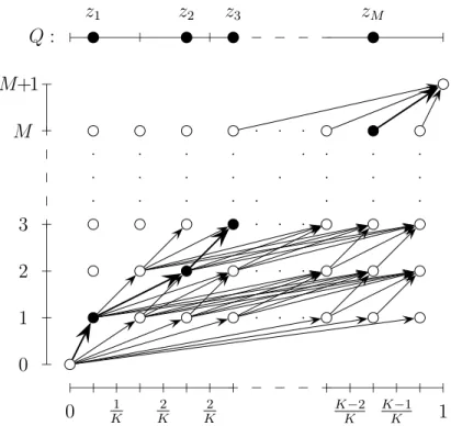
Consider an acyclic directed graph (V,E), where V and E denote the set of vertices and edges, respectively. Given a fixed pair of vertices s and u, let R denote the set of all directed paths from s tou, and assume that Ris not empty. We also assume that for all z 6=u,z ∈ V, there is an edge starting from z. (Otherwise vertex z is of no use in finding a path froms tou, and all such vertices can be removed iteratively from the graph at the beginning of the algorithm inO(|V|) +O(|E|) time.) Finally, we assume that the vertices are labeled by the integers 1,2, . . . ,|V|such thats = 1,u=|V|, and ifz1 < z2, then there is no edge from z2 to z1 (such an ordered labeling can be found in O(|E|) time since the graph is acyclic). At time t= 1,2, . . . the predictor picks a path ˆyt∈ R. The cost of this path is the sum of the weights δt(a) on the edges a of the path (the weights are assumed

(18)

to be nonnegative real numbers), which are revealed for each a ∈ E only after the path has been chosen. To use our previous definition for prediction in Section 2, we may define yt={δt(a)}a∈E, and the loss function

`(yt,yˆt) = X

a∈yˆt

δt(a)

for each pair (yt,yˆt). The cumulative loss at timeT is given by LT =

XT t=1

`(yt,yˆt).

Our goal is to perform as well as the best combination of paths (experts) which is allowed to change the pathmtimes during the time intervalt= 1, . . . , T. As in the prediction context, such a combination is given by an m-partition P(T, m,t,e), wheret = (t1, . . . , tm) such that t0 = 0 < t1 < · · ·< tm < tm+1 =T, and e = (e0, . . . , em), where ei ∈ R (that is, expert e∈ R predicts ˆy_t^(e)=e). The cumulative loss of a partition P(T, m,t,e) is

L(P(T, m,t,e)) = Xm

i=0 ti+1

X

t=ti+1

`(y_t, e_i) = Xm

i=0 ti+1

X

t=ti+1

X

a∈ei

δ_t(a).

Now Algorithms 1 and 2 can be used to choose the path ˆytrandomly at each time instant t= 1, . . . , T, and the regret

LT −min

t,e L(P(T, m,t,e))

can be bounded by Theorem 1. In this setup, with the aid of the weight pushing algorithm [11, 12, 13], we can compute efficiently a path based on the exponentially weighted prediction method and the constants Zt⁰,t, and thus prove the following theorem.

Theorem 4 For the minimum-weight path problem described in this section, Algorithm 2 can be implemented in O(T²|E|) +O(T³) time. Moreover, let N denote the number of different paths from vertexsto vertexu, and assume thatα= _T^m₋₁ <1,δt(a)< B/(|V|−1) for all t and edges a ∈ E, and η is chosen according to (6). Then for any p∈ (0,1), the regret of the algorithm can be bounded from above, with probability at least 1−p, as

LT −min

t,e L(P(T, m,t,e))

≤ T^1/2 B

√2 r

(m+ 1) lnN +mlnT −1

m +m+B

rT ln(1/p)

2 .

The expected regret of the algorithm can be bounded as EL_T −min

t,e L(P(T, m,t,e))

≤ T^1/2 B

√2 r

(m+ 1) lnN +mlnT −1 m +m.

(19)

Proof. The performance bound in the theorem follows trivially from the optimized bound (7) in Theorem 1. All we need to show is that the algorithm can be implemented in O(T²|E|) +O(T³) time. To do this, we first revisit the weight pushing algorithm [11, 12, 13] via a modification of the algorithm of [14] for choosing a path ˆyt randomly based on (yt⁰, yt⁰+1, . . . , yt−1). That is, based on the weights {δi(a)}a∈E, i ∈ [t⁰, t−1], we have to choose a path ˆyt according to the probabilities

P{yˆt=r}= e^−η^P^a∈r^∆^t⁰^,t−1^(a) P

r⁰∈Re^−η^P^a∈r⁰^∆^t⁰^,t−1^(a) (24)

where ∆t⁰,t−1(a) = Pt−1

i=t⁰δi(a), and compute Zt⁰,t−1 =X

r∈R

e^−η^P^a∈r^∆^t⁰^,t−1^(a).

Using the constants Z1,t−1, . . . , Zt−1,t−1 and W1, . . . , Wt−1, we can compute Wt, and perform the random choice of τt via Algorithm 2. In what follows we show how these steps can be done efficiently.

For any z ∈ V, let Rz denote the set of paths from z to u (we define Ru = ∅), and let Gt⁰,t(z) denote the sum of the exponential cumulative losses in the interval [t⁰, t] of all paths in Rz. Formally, if Rz is empty then we define Gt⁰,t(z) = 1, otherwise

G_t⁰_,t(z) = X

r∈Rz

e^−η^P^a∈r^∆^t⁰^,t^(a). (25) ThenZ_t⁰_,t=G_t⁰_,t(s), andG_t⁰_,t(z) can be computed recursively forz =u−1, u−2, . . . , s= 1, as G_t⁰_,t(u) = 1,

G_t⁰_,t(z) = X

ˆ z:(z,ˆz)∈E

e^−η∆^t⁰^,t^((z,ˆ^z))G_t⁰_,t(ˆz). (26) Note that since ˆz > z if (z,z)ˆ ∈ E, Gt⁰,t(ˆz) is already available when it is needed in the above formula. In the recursion each edge is taken into consideration exactly once.

Therefore, calculating Gt⁰,t(z) for all z ∈ V requires O(|E|) computations for any fixed 1≤ t⁰ ≤ t, provided the cumulative weights ∆t⁰,t(a) are known for all edges a ∈ E. Now for a given t, as t⁰ is decreased fromt to 1, if we store the cumulative weights ∆t⁰,t(a) for each edge a, then only O(|E|) computations are needed to update the cumulative weights at the edges for each t⁰. Therefore, for a given t, calculating Gt⁰,t(z) for all z ∈ V and 1≤t⁰ ≤t requires O(t|E|) computations.

The function Gt⁰,t−1 offers an efficient way of drawing ˆyt randomly for a givenτt=t⁰: For any z∈ V \ {u}, let E^z ={zˆ: (z,z)ˆ ∈ E} and

p_t⁰_,t(ˆz|z) =e^−η∆^t⁰^,t−1^((z,ˆ^z))G_t⁰_,t−1(ˆz)

G (z), zˆ∈ Ez.

(20)

For fixed z, pt⁰,t(ˆz|z) is a probability distribution onEz since by (25) X

ˆ z∈Ez

pt⁰,t(ˆz|z) = 1.

Denote the kth vertex along a path r ∈ R by zr,k for k = 0,1, . . . ,|r|, where |r| is the length of the path r (zr,0 =s and zr,|r|=u). Then,

Y|r|

k=1

pt⁰,t(zk,r|zk−1,r) = Y|r|

k=1

e^−η∆^t⁰^,t−1^((z^k−1,r^,z^k,r⁾⁾ Gt⁰,t−1(zk,r) Gt⁰,t−1(zk−1,r)

= e^−η^P^|r|^k=1^∆^t⁰^,t−1^((z^k−1,r^,z^k,r⁾⁾Gt⁰,t−1(u) Gt⁰,t−1(s)

= P{yˆt =r} (27)

by (24) sinceGt⁰,t−1(u) = 1 andGt⁰,t−1(s) =P

r⁰∈Re^−η^P^a∈r⁰^∆^t⁰^,t^(a). Thus ˆyt can be drawn randomly in a sequential manner: Starting fromzyˆt,0 =s, in each stepk = 1,2, . . .choose z =zyˆt,k randomly fromE^zyt,kˆ −1 with probabilitypt⁰,t(z|zyˆt,k−1). The procedure stops when zyˆt,k =u. Thus ˆyt can be computed inO(|V|) steps ifτt=t⁰ and the functions ∆t⁰,t−1 and Gt⁰,t−1 are given, as any path from s to r is of length at most |V| −1.

It remains to show that τt can be chosen efficiently. As we have seen before, Gt⁰,t(z) can be computed in O(t|E|) time for all z and 1 ≤ t⁰ ≤ t; hence finding Zt⁰,t = Gt⁰,t(s) requires O(t|E|) computations. Then, given Wt⁰ for t⁰ = 1, . . . , t, Wt+1 can be computed by (10) in O(t) steps, and so for all t⁰ = 1, . . . , t, the computational time of Wt⁰ and Zt⁰,t is O(t|E|) +O(t²). Therefore, τt can be chosen randomly according to (13) in the same computational time. Finally, as we have seen in the preceding paragraph, given τt=t⁰ and the function Gt⁰,t, ˆyt can be computed in O(|V|) steps. Thus, the overall time complexity of computing ˆyt for a givent isO(t|E|) +O(t²) +O(|V|) = O(t|E|) +O(t²) (as

|E| ≥ |V| −1). Thus, Algorithm 2 can be performed in O(T²|E|) +O(T³) time.

5 Online scalar quantization

In this section we apply the results of Sections 3 and 4 to construct efficient zero-delay sequential source codes. Our goal is to find efficiently implementable zero-delay coding schemes which perform asymptotically as well as the best scalar quantization scheme which is allowed to change the employed quantizer a certain number of times.

We assume that the source and reconstruction symbols belong to the interval [0,1].

Then a zero-delay scheme using encoder randomization is given formally by the encoder- decoder functions{fi, gi}^∞i=1, where

fi : [0,1]ⁱ×[0,1]ⁱ → {1,2, . . . , M}