Universidad Católica San Pablo: Unsupervised anomaly detection in 2D radiographs using generative models

(1)

Unsupervised anomaly detection in 2D radiographs using generative models

Laura Jovani Estacio Cerqu´ın

Advisor: PhD. Rensso Mora Colque Co-Advisor: PhD. Hans Lamecker

Committee Members:

PhD. David Menotti – Universidade Federal do Paran´a, Brazil PhD. Javier Montoya Zegarra – ETH-Zurich, Switzerland

PhD. Guillermo Cámara Chávez – Universidade Federal do Ouro Preto, Brazil PhD. José Eduardo Ochoa-Luna – Universidad Católica San Pablo, Peru

Thesis submitted to the Department of Computer Science

in partial fulfillment of the requirements for the degree of Master in Computer Science.

Universidad Cat´olica San Pablo – UCSP June of 2022 - Arequipa – Peru

(2)

(3)

To God for guiding my life.

To my parents, Catalina and Jose, who support and encourage me to accomplish my dreams.

(4)

Abbreviations

2D Two-dimensional

3D Three-dimensional

AAE Adversarial Autoencoder

AE Autoencoder

ANODE09 Automatic Nodule Detection 2009

AP Anteroposterior

AUC Area Under the Curve

BPNN Backpropagation Neural Network

BRATS Multimodal Brain Tumor Image Segmentation Benchmark

CNN Convolutional Neural Network

CDC Centers for Disease Control and Prevention

CT Computed Tomography

DCGAN Deep Convolutional Generative Adversarial Network

DCNN Deep Convolutional Neural Network

III

(5)

DICOM The Digital Imaging and Communications in Medicine

DRRs Digitally reconstructed radiographs

ED Emergency Department

f-AnoGAN Fast AnoGAN

FCN Fully Convolutional Network

FD Fr´echet Inception Distance

FROC Free-response Receiver Operating Characteristic Curve

GAN Generative Adversarial Network

HU Hounsfield Unit

ICAC Carotid Artery Calcification

ISBI International Symposium on Biomedical Imaging

ISLES Ischemic Lesion

KL Kullback-Leibler

KNN K-Nearest Neighbors

LDCT Low Dose Computed Tomography

MAE Mean Absolute Error

MICCAI Medical Image Computing and Computer Assisted Intervention

(6)

MRI Magnetic Resonance Imaging

MSE Mean Squared Error

OCT Optical Coherence Tomography

PCA Principal Component Analysis

PDF Probability Density Function

PSNR Peak Signal-to-Noise Ratio

RF Random Forest

ROC Receiver Operating Characteristics

SAGAN Sharpness-aware generative adversarial network

SGD Stochastic Gradient Descent

SSD Sum of Squared Differences

SSIM Structural Similarity Index

SWI Susceptibility-weighted Imaging

SSM Statistical Shape Model

TB Tuberculosis

VAE Variatonal Autoencoder

WGAN Wasserstein GAN

Master Program in Computer Science - UCSP V

(7)

(8)

Acknowledgments

First of all, I wish to thank PhD. Rensso Mora and PhD. Hans Lamecker, my advisors who introduced me in the research field of machine learning to solve real problems in the medical field. Their constant support made this work possible. I am truly grateful with PhD. Moritz Ehlke; his support providing me with suggestions and sharing his knowledge have been an inspiration for me.

I wish to thank PhD. Stefan Zachow for his valuable feedback and support in this research work. I am grateful with PhD. Alexander Tack for his support verifying the code and giving me recommendations to solve some errors. This work has been supported by helpful reviews from colleagues in the scientific community, to whom I owe my gratitude for appraising my work critically. I am also grateful with PhD.

Eveling Castro, head of the CiTeSoft-UNSA for the database access.

I would like to thank in a special way the National Council for Science, Technology and Technological Innovation (CONCYTEC-PERU) and the National Fund for Scientific and Technological Development and Technological Innovation (FONDECYT-CIENCIACTIVA), which through the Management Agreement 234-2015-FONDECYT have allowed the grant and financing of my studies in the Master Program in Computer Science at Universidad Cat´olica San Pablo (UCSP).

VII

(9)

(10)

Abstract

We present a method based on a generative model for detection of anomalies such as prosthesis, implants, screws, zippers, and metals in Two-dimensional (2D) radiographs. The generative model is trained following an unsupervised fashion using clinical radiographs as well as simulated data neither of them containing anomalies. Our approach employs a reconstruction loss and a latent space consistency loss which have the benefit of identifying similarities which forced to reconstruct X-rays without anomalies.

In order to detect images with anomalies, an anomaly score is also computed employing the reconstruction loss and the latent space consistency loss. Additionally, the Fr´echet distance is introduced as part of the reconstruction loss. These losses are computed between an input X-ray and the one reconstructed by the proposed generative model. Validation was performed using clinical pelvis radiographs. We achieved an Area Under the Curve (AUC) of 0.77 and 0.83 with clinical and synthetic data, respectively. The results demonstrated a good accuracy of the proposed method for detecting outliers as well as the advantage of utilizing synthetic data for the training stage.

keywords: Anomaly Detection, Unsupervised Learning, Generative Adversarial Networks, Pelvic radiographs.

IX

(11)

(12)

Resumen

Presentamos un método basado en un modelo generativo para la detección de anomal´ıas tales como prótesis, implantes, tornillos, cremalleras y metales en radiograf´ıas en 2D. El modelo generativo se entrena de forma no supervisada utilizando radiograf´ıas cl´ınicas as´ı como datos simulados que no contienen anomal´ıas. Nuestro enfoque emplea una pérdida de reconstrucción y una pérdida de consistencia del espacio latente que tienen la ventaja de identificar similitudes que obligan a reconstruir radiograf´ıas sin anomal´ıas.

Con la finalidad de detectar imágenes con anomal´ıas, también se calcula una puntuación de anomal´ıas utilizando la pérdida de reconstrucción y la pérdida de consistencia del espacio latente. Adicionalmente, se introduce la distancia Fréchet como parte de la pérdida de reconstrucción.

Estas pérdidas se calculan entre una radiograf´ıa de entrada y la radiograf´ıa reconstruida por el modelo generativo propuesto. La validación se realizó utilizando radiograf´ıas cl´ınicas de la pelvis. Se alcanzó un AUC de 0,77 y 0,83 con datos cl´ınicos y sintéticos, respectivamente. Los resultados demostraron una buena precisión del método propuesto para detectar anomal´ıas, as´ı como la ventaja de utilizar datos sintéticos para la etapa de entrenamiento.

Palabras clave: Detecci´on de anomal´ıas, Aprendizaje no supervisado, Redes generativas adversarias, radiograf´ıas p´elvicas.

XI

(13)

(14)

List of Tables

3.1 Publications based on hand-crafted features. . . 39

3.2 Publications based on supervised learning. . . 42

3.3 Publications based on unsupervised learning: Autoencoders and Variational Autoencoders. . . 45

3.4 Publications based on unsupervised learning: Generative Adversarial Networks. . . 49

5.1 AUC scores. All methods are trained on clinical data . . . 66

5.2 AUC scores. All methods are trained on synthetic data. . . 67

5.3 AUC scores. Experiment using clinical data. . . 67

5.4 AUC scores. Experiment using synthetic data. . . 67

XVII

(19)

LIST OF TABLES

(20)

List of Figures

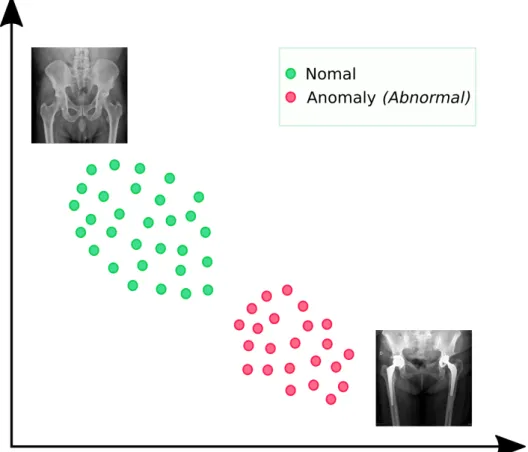
1.1 Latent space representation. X-ray imaging is encoded into a latent space. Green circles represent normal X-rays and pink circles represent X-rays with anomalies. In an ideal case, normal X-rays and abnormal X-rays can be mapped separated in the latent space; however, this does not happen in real applications. . . 4 1.2 General Overview. The main contribution of our work is presented

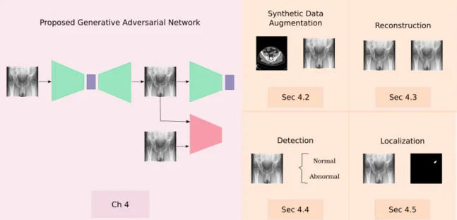
in Chapter 4. The method was designed for the application of medical images with the objective of detecting anomalies following an unsupervised learning approach. . . 5 1.3 Overview of the reconstruction pipeline. Steps 2 and 3 are based on

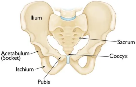
adjusting the Statistical Shape Model (SSM), whereas step 4 is based on an unsupervised Generative Adversarial Network (GAN). . . 6 2.1 Pelvic structure anatomy. Source: Britannica(2011). . . 10 2.2 Foreign body ingestion. This kind of anomaly in adults is typically

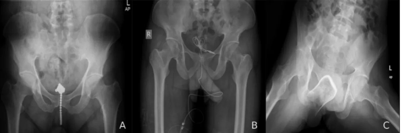
accidental. However, the image demonstrates numerous thumb tacks ingested in a suicide attempt. Source: Image courtesy of Lars Grimm, MD, MHS. . . 12 2.3 Pelvic X-ray in anteroposterior view. . . 13 2.4 Examples of foreign objects in the pelvis. A) Plain radiograph of the

pelvis showing a dense metallic foreign body that was composed of many small magnetic balls in the pelvic region, of which one part was a cloddy body in the bladder and the other part was a long-striped body in the posterior urethra (Li et al.,2018). B) Plain radiograph that shows an ear phone cable within the bladder. This is a clear X-ray example depicting radiopaque foreign body within bladder (Hegde et al., 2018). C) Plain radiograph showing a glass bottle at the beginning of the upper-middle region of the rectum and extending to the anal verge, and its open edge was directed to the bottom, and its base was proximal, on standing (Ozbilgin et al., 2015). . . 14

XIX

(21)

LIST OF FIGURES 2.5 Anomaly types. A) Point anomaly: represented by A₁, A₂, A₃; these

points are outside from the normal clusters N₁ and N₂. B) Contextual anomaly: represented by the low value of temperature. This pattern is anomalous because it differs from the periodic context. C) Collective anomaly: represented by the horizontal pattern half way along the graph.

This pattern is anomalous when compared to previous normal patterns.

Source: Image reproduced from (Araya,2016). . . 17

2.6 Supervised anomaly detection illustration. . . 18

2.7 Semi-supervised anomaly detection illustration. . . 19

2.8 Unsupervised anomaly detection illustration. . . 19

2.9 Anomalies in the pelvis. Anomalies in the pelvic bone have variable shapes and appearances. For instance, only paying attention to the nails they have variable length, location and silhouette. Moreover, nails lose their shape when they are overlapping with other structures such as implants. . . 20

2.10 The Kullback-Leibler (KL) divergence is asymmetric. Suppose we have a distributionp(x) and wish to approximate it with another distribution q(x). Therefore, we have the choice of minimising either D_KL(p||q) or D_KL(q||p). (Left) The effect of minimisingD_KL(p||q). (Right) The effect of minimising D_KL(q||p). Source: Image extracted from (Goodfellow et al., 2016). . . 23

2.11 The normal distribution (Goodfellow et al., 2016). The normal distribution N(x;µ, σ²) exhibits a classic “bell curve” shape, with the x coordinate of its central peak given by µ, and the width of its peak controlled byσ. In this example, thestandard normal distribution, with µ= 0 andσ = 1. . . 23

2.12 Autoencoder model. . . 25

2.13 The graphical model involved in a variational autoencoder. Solid lines denote the generative distribution pθ(.) and dashed lines denote the distribution q_ϕ(z|x) to approximate the intractable posterior p_θ(z|x). . 26

2.14 Illustration of the variational autoencoder architecture. . . 27

2.15 Illustration of generative adversarial network architecture. . . 29

2.16 Illustration of adversarial autoencoder architecture. . . 31 2.17 Area under the curve. The Receiver Operating Characteristics (ROC)

curves of two score classifiers are shown. The AUC for classifier B is shown as a dark gray-filled area. The AUC for classifier A corresponds to the light gray-filled area plus the dark gray-filled area (Melo,2013) . 35

(22)

LIST OF FIGURES

3.1 Anomaly detection framework. Both steps of model training, generative adversarial training (yields a trained generator and discriminator) and encoder training (yields a trained encoder), are performed on normal (healthy) data and anomaly detection is performed on both unseen healthy cases and anomalous data (Schlegl et al., 2019). . . 47

4.1 Flowchart of the anomaly detection process. It consists of four stages:

synthetic data augmentation, reconstruction, detection and localization. 54 4.2 Illustration of the difference between visualising a Three-dimensional

(3D) data volume and a DRR rendered from a 3D data volume using a ray casting method. a) illustrates a ray casting method for rendering a surface from a 3D volume, b) illustrates a ray casting method for rendering a DRR from 3D volume data, (c) illustrates an example of a surface rendered from volume data (Ehlke et al.,2013), and d) illustrates an example of a DRR. . . 56 4.3 Proposed GAN architecture for detecting anomalies. x_i and ˆx_i represent

the input image and the reconstructed image, whereasz_iand ˆz_irepresent the latent space of the input and the reconstructed image, respectively.

G_E, D and E are convolutional networks and G_D is a deconvolutional network. . . 57 4.4 Detection of anomalies in X-rays. Given a new image in the testing

stage, it is passed through the generator and the encoder in order to obtain the losses for the anomaly score function. . . 59 4.5 General overview of the anomaly localization process. A simple

subtraction between the input X-ray image x_j and the reconstructed X-ray image ˆx_j is applied to get the anomaly localization.. . . 60

5.1 Kinds of anomalies in the pelvis.. . . 64 5.2 Receiver operating characteristics for the clinical experiment. . . 68 5.3 Receiver operating characteristics for the synthetic experiment.. . . 68 5.4 Reconstruction of clinical pelvic X-rays. The methods were trained using

clinical data. The first two rows are pelvic X-rays with anomalies and the last two rows are pelvic X-rays without anomalies. . . 69 5.5 Reconstruction of clinical pelvic X-rays. The methods were trained using

synthetic data. The first two rows are pelvic X-rays with anomalies and the last two rows are pelvic X-rays without anomalies. . . 70

Master Program in Computer Science - UCSP XXI

(23)

LIST OF FIGURES 5.6 Pixel-level localization of anomalies in clinical pelvic X-rays. The

methods were trained using clinical data. The first two rows are pelvic X-rays with anomalies and the last two rows are pelvic X-rays without anomalies. . . 71 5.7 Pixel-level localization of anomalies in clinical pelvic X-rays. The

methods were trained using synthetic data. The first two rows are pelvic X-rays with anomalies and the last two rows are pelvic X-rays without anomalies. . . 72 5.8 Reconstruction comparison. Green lines represent the distance of the

input X-ray at different positions. Red lines represent faulty distances of the different methods. Finally, green ellipses are just to note the border (white lines) in this region. . . 74 5.9 Example of region of interest of anomalies in clinical pelvic X-rays. The

first row represents the ground-truth localization. The second and third rows represent the output of our method. . . 75 6.1 3D reconstruction example from two X-ray images. The reconstructed

anatomy is obtained from anteroposterior view and lateral view X-ray images (Ehlke et al., 2013) . . . 79

(24)

Chapter 1 Introduction

1.1 Motivation

Anomaly detection is the process of finding abnormal patterns from a given dataset (Hawkins, 1980; Chandola et al., 2009). These patterns belong to data with large deviations due to being previously absent or overlooked. This area has been of increasing importance as a result of the need to efficiently detect these abnormal patterns to support decision-making systems (Chalapathy and Chawla, 2019).

Consequently, anomaly detection plays an important role in the development of many applications in several fields of study such as video surveillance (Feng et al., 2017), manufacturing damage detection (Liu et al., 2018), detection of fraudulent usage of credit cards (Tran et al., 2018), detection of failures in cyber-security (Goh et al., 2017), and disease detection (Baur et al., 2018).

The anomaly detection task in the medical field involves identifying abnormal patterns that are different from the bone structures or soft tissues inherent to the human body. In this regard, foreign object detection in X-ray imaging is an ongoing research problem of high impact due to it being a common cause of visits to emergency departments (Tseng et al., 2015). Foreign objects can gain entry to the human body through a variety of methods, including ingestion, aspiration and surgical interventions (Hunter and Taljanovic,2003; Cinar et al., 2018). Therefore, depending on the foreign object, they can produce infections or neoplasms and serious complications causing morbidity or mortality (Boppana et al., 2014; Kasotakis et al., 2012). Furthermore, these anomalies hinder the performance of applications focused on the automated processing of X-rays from the screening process to disease detection (Zohora and Santosh,2016).

In previous work, machine learning approaches have been proposed as the solution to anomaly detection tasks in X-ray imaging(Agrawal and Agrawal, 2015).

1

(25)

1.1. Motivation These approaches are mainly divided into two categories, supervised learning and unsupervised learning (Hodge and Austin,2004;Ukil et al.,2016). Supervised learning requires a large set of labelled training dataset to build a discriminate model that classifies X-ray imaging into normal and abnormal. However, it is not always possible to get labels or annotations for all kinds of anomalies since some of them are very rare in shape and texture, and can occur spontaneously as novelties during the test phase (Ahmed et al., 2016; Schlegl et al., 2017). In other words, these methods suffer some deficiencies: (1) a restricted number of labeled or annotated training datasets due to their acquisition being tedious, prone to error and a time-consuming task, (2) they require training datasets of normal and abnormal samples, and (3) they are limited to known shapes and textures of foreign objects. All these factors make the learning process difficult to be representative for all possible scenarios.

Hence, supervised learning methods can produce faulty outputs when they receive an unexpected input. This imprecise output can affect the decision-making process leading to wrong conclusions being made when using automated tools for detection or diagnosis decision purposes.

On the other hand, a more consistent solution has been proposed to tackle these drawbacks based on unsupervised learning methods. Contrary to supervised learning, unsupervised learning is able to identify unexpected shapes or textures in datasets, which differ from the data distribution (intrinsic properties from normal X-ray imaging dataset) over which they were trained on; and most important, they do not require labeled or annotated datasets of normal and abnormal samples (Schlegl et al., 2017; Goldstein and Uchida, 2016). Although unsupervised anomaly detection can in principle also be applied to other anatomies and medical imaging modalities, we focus on foreign object detection in pelvic X-rays of Anteroposterior (AP) view due to their valuable importance in automated processing applications (Zohora and Santosh,2016) such as reporting critical findings in emergency interventions (Xue et al., 2015;Welton et al.,2018;Tseng et al.,2015) and 3D anatomy reconstruction from X-rays(Vikas and Ravi,2014; Ehlke et al., 2013).

These applications require identifying important features in the images. Hence, in case the features are not visible due to the presence of foreign objects such as implants or due to the absence of a part of the anatomy in the images, the 3D reconstruction could be inaccurate (Melhem et al., 2016; Yu et al., 2016). In such cases, generating images without these anomalies or identifying them could be helpful for segmentation and registration tasks required to develop biomedical applications.

However, in spite of its importance, it possesses some challenging problems to address.

First, foreign objects (anomalies) have variable and unknown shape and texture because of several factors such as silhouette, material and location (Tseng et al., 2015). Second, the dynamic nature of anomalies makes it challenging to have labels or annotations (Schlegl et al., 2017; Akcay et al., 2018). Third, since the X-ray imaging lacks high resolution they have variable levels of contrast, which make the anomalies identification difficult (Tseng et al.,2015;Xue et al.,2015).

Therefore, the fundamental hypothesis pursued in this thesis, is that all of these

(26)

CHAPTER 1. Introduction

problems can be solved using generative models in order to detect abnormal patterns present on the X-ray images taking into account a training dataset of normal X-rays. In other words, this strategy is based on the learning of the prior distribution of normal X-ray images. To this purpose, we focus on generative models such as GAN that have two main components: (1) a generative model which generates new samples based on a reduced number of high level features known as latent space, and (2) a discriminative model which discriminates between different kinds of data instances.

We believe this model is able to reconstruct normal X-rays and it has limitations to reconstruct abnormal ones since they were unseen by the model in the training phase.

1.2 Problem

Despite the success ofGAN in many applications, one of the major concerns is the fact that GAN-based anomaly detection has two main challenges in the medical field: (1) there is not a large dataset for the training stage that covers all variabilities in the data, and (2) there is no anomaly score which also computes the visual quality of the images to determine the presence or absence of an anomaly. These two drawbacks prevent the learning of high-level representative features that ensure adequate reconstruction and detection, on which we focus our interest.

1.3 Goals

To address the aforementioned problems, our research work pursues the following goals:

Overall Goal

• Detect anomalies in 2D pelvic X-ray images of anteroposterior view following an unsupervised approach based on generative adversarial networks.

Specific Goals

• To propose a strategy for synthetic data generation that allows to overcome the inaccurate reconstruction of X-ray images due to a small amount of data for the training stage.

• To propose an unsupervised learning method based on generative adversarial networks which allows to reconstruct realistic samples without anomalies to facilitate the anomaly detection process.

• To introduce a different loss function into the anomaly score which facilitates the detection and localization of anomalies based on the reconstruction quality, Master Program in Computer Science - UCSP 3

(27)

1.4. Method the consistency in the high level features, and the visual quality of the generated samples.

• To analyze the results of the proposed unsupervised anomaly detection method in2Dpelvic X-ray imaging of anteroposterior view comparing its performance to related work approaches.

1.4 Method

Recently, unsupervised anomaly detection is addressed using generative models such as adversarial autoencoders or generative adversarial networks. These methods propose to learn the data distribution from normal images in the training stage, and then to be able to discriminate images that do not have the same data distribution in the testing stage (see Figure 1.1).

Figure 1.1: Latent space representation. X-ray imaging is encoded into a latent space.

Green circles represent normal X-rays and pink circles represent X-rays with anomalies.

In an ideal case, normal X-rays and abnormal X-rays can be mapped separated in the latent space; however, this does not happen in real applications.

The anomaly detection task using generative adversarial neural networks can be addressed from two perspectives. The first one is focused on the generative aspect, which tries to identify the structure of the training samples in order to generate new

(28)

similar samples. The second one is focused on the discriminative aspect which uses the discriminator network to learn the distribution of normal samples with the aim to identify anomalies.

Our proposal considers the two aspects merged into one. The generative aspect relies on the strength of GANs to reconstruct images similar to the training samples.

Then, in the discriminative aspect, we use an anomaly score based on the reconstruction loss, consistency of the high level features and visual quality of the generated samples to identify an X-ray as normal or abnormal. In this regard, the discriminator information is just used as a regularizer to generate realistic samples, thus depending on the discriminator network loss, the generated X-rays will be of high-quality (normal X-rays) or poor-quality (abnormal X-rays). The use of the generative aspect in our proposal is made by the assumption that X-rays with anomalies will be reconstructed as normal ones such that we can roughly localize the anomalies applying a simple subtraction between the original X-ray and the reconstructed X-ray. A general overview of the proposed method is shown inFigure 1.2.

Figure 1.2: General Overview. The main contribution of our work is presented in Chapter 4. The method was designed for the application of medical images with the objective of detecting anomalies following an unsupervised learning approach.

Master Program in Computer Science - UCSP 5

(29)

1.5. Contributions

1.5 Contributions

The main contributions of this work are presented as follows:

• Unsupervised Anomaly Detection: We propose an unsupervised method which only requires exemplary data of expected inputs in the training stage to detect unexpected inputs as anomalies in the testing stage. It demonstrates superior results against current GAN-based and traditional autoencoder-based approaches.

• Synthetic Data Augmentation: We present a strategy for synthetic data generation using Digitally reconstructed radiographs (DRRs) to cover an even larger population with the aim to improve the prediction accuracy in our experiments.

• Anomaly Score: We introduce a score of anomalies detection based on the reconstruction and the contextual loss that allows improving the prediction accuracy.

• Research Contribution as Author: The proposed method was accepted and presented in the IEEE International Symposium on Biomedical Imaging (ISBI) 2021, which is the second most important conference in the medical field.

• Research Contribution as Co-Author: The proposed method was also validated as post-processing stage in the Medical Image Computing and Computer Assisted Intervention (MICCAI) 2020 Cranial Implant Design Challenge to remove smaller, localized defects in volumes of the skull (see Figure 1.3). In this regard, we obtained the best paper award in the MICCAI challenge. Subsequently, an extension of the paper was published in the IEEE Transactions on Medical Imaging journal.

Figure 1.3: Overview of the reconstruction pipeline. Steps 2 and 3 are based on adjusting the SSM, whereas step 4 is based on an unsupervisedGAN.

(30)

1.6 Outline

This research work is structured as follows: InChapter 2we presented the background information on X-ray imaging of pelvic structure, generative models and generative adversarial networks that help to a better understanding of the topic. InChapter 3 we introduced the related work about several unsupervised anomaly detection methods in the medical field. We discussed their performance and limitations according to their proposed approaches.

Chapter 4 presents our methodology to address unsupervised anomaly detection in 2D radiographs of the pelvic bone. Here, the generative adversarial network architecture and the stages to detect anomalies are explained in detail. The experiments are presented in Chapter 5, we describe the reconstruction and the anomaly detection results based on a qualitative analysis. Moreover, we discussed the quantitative results based on theAUC for the detection stage. Finally, Chapter 6 exposes the conclusions and future work based on our proposed goals.

(31)

1.6. Outline

(32)

Chapter 2 Background

The anomaly detection task in medical imaging involves different areas of study from the medical to the computing fields. From the medical point of view, it is important to know the anatomy of the bone or soft tissue analysed using radiological modalities to find anomalies in them. On the other hand, from the computational point of view, the anomaly detection task requires the confluence of several methods from related areas such as deep learning or machine learning. Moreover, once an anomaly is detected using these methods, a crucial step is to evaluate their performance using some metrics focused on this task. Therefore, this chapter is devoted to detailing some background knowledge of critical related areas for a better understanding of the whole research work.

Section 2.1 describes biomedical concepts about the pelvic structure, the main anomalies associated with it, and the radiological modalities to analyse these anomalies.

Section 2.2 introduces the anomaly detection problem and the approaches to solve it.

The most promising methods for unsupervised anomaly detection are explained in Section 2.3. Finally, a general description of metrics for evaluating the final results are presented in Section 2.4.

2.1 Biomedical Concepts

The biomedical concepts section is the starting point to understand the anatomical structure that this research work is focused on. First, the anatomy of the pelvic bone is presented to know its importance and function in the human body. Then, the most common anomalies in the pelvis are described. Even though the term anomaly in the medical field is more related to pathologies, it also refers to foreign objects as we mentioned in the first chapter. Finally, the radiological modalities such as Magnetic Resonance Imaging (MRI), Computed Tomography (CT), and X-rays are presented.

It is important to mention that we extended the background that is more useful for us.

For instance, we emphasise the review of pelvic anomalies and radiological modalities 9

(33)

2.1. Biomedical Concepts in terms of foreign objects and X-rays respectively.

2.1.1 Pelvic Structure Anatomy

The pelvis consists of paired hipbones, connected in front of the back pubic symphysis by the sacrum (see Figure 2.1). Each pair is made up of three bones: (1) the blade-shaped ilium, above and to either side, which accounts for the width of the hips. (2) The ischium, behind and below, on which the weight falls on sitting. (3) The pubis, in front. All three unite in early adulthood at a triangular suture in the acetabulum, the cup-shaped socket that forms the hip joint with the head of the femur (thighbone). The ring made by the pelvis functions as the birth canal in females.

The pelvis provides attachment for muscles that balance and support the trunk and move the legs, the hips, and the trunk. In the human infant, the pelvis is narrow and non-supportive. As the child begins walking, the pelvis broadens and tilts, the sacrum descends deeper into its articulation with the ilia, and the lumbar curve of the lower back develops (Moore and Dalley, 2009).

Sex differences in the pelvis are marked and reflect the necessity in the female for providing an adequate birth canal for a large-headed fetus. In comparison with the male pelvis, the female basin is broader and shallower. The birth canal is rounded and capacious. The sciatic notch wide and U-shaped. The pubic symphysis short, with the pubic bones forming a broad angle with each other. The sacrum short, broad, and only moderately curved. The coccyx movable, and the acetabulum further apart. Those differences reach their adult proportions only at puberty (Latarjet and Liard, 2006).

Figure 2.1: Pelvic structure anatomy. Source: Britannica(2011).

(34)

CHAPTER 2. Background

2.1.2 Anomalies in the Pelvic Structure

The pelvic bone is prone to suffering from different anomalies as an effect of the accidents or the patient’s age. The main anomalies that affect the pelvis are related to pelvic trauma, tumours or foreign objects that obstruct the proper analysis of this structure. We describe these kinds of anomalies, highlighting the foreign objects because they are the case of study in this research work.

Trauma.- It constitutes one of the most complex problems of bone structures and occurs in 3% of skeletal injuries (Coccolini et al., 2017). According to the Centers for Disease Control and Prevention (CDC), trauma injuries kill more people between the ages of 1 and 44 than any other disease. Localised fractures in the pelvic structure are of high incidence (S´anchez, 2014) and are often caused by traffic accidents, falls or sports accidents. Moreover, they occur together with multiple injuries in other bodily locations associated with high mortality and disability rates (Cai et al., 2017;

Karadimas et al., 2011). The mortality rate being 8.6% to 50% (Wu et al., 2012).

Tumours.- Patients with pelvic tumours are usually elderly, and their tumours are larger relative to patients with tumours in extremities. The majority of tumours in the pelvis are malignant, while those in the extremities (proximal femur) are in their majority benign (Bloem and Reidsma, 2012). Soft tissue masses in the thigh in the elderly are typically sarcomas without tumour specific signs. Common tumour-like lesions occurring in the hip and pelvis that can mimic neoplasm are: infections (including tuberculosis), insufficiency/avulsion fractures, cysts, fibrous dysplasia, aneurysmal bone cyst, Langerhans cell histiocytosis, and Paget’s disease (Scheitza et al., 2016). Clinically, the main difference is that pelvic tumours are located deep in the body, while tumours located in the extremities are relatively superficial. Typically, pelvic tumours are detected several years later compared to the same tumour type located in the extremities (Park et al., 2017).

Foreign Objects.- Foreign objects or foreign bodies are a common cause of visits to the Emergency Department (ED), and can gain entry to the human body through a variety of methods, including ingestion, aspiration, and purposeful insertion (Tseng et al., 2015). They can produce infections or neoplasms and serious complications causing morbidity or mortality (Boppana et al., 2014). Foreign body ingestions or insertions are seen in four broad categories of patients: (1) children, (2) mentally handicapped or mentally retarded people, (3) adults with unusual sexual behaviour, and (4) “normal” adults or children with predisposing factors or injurious situational problems. This latter group includes individuals who may abuse drugs or alcohol, engage in criminal activities, engage in extreme sporting activities, or may be subject to child or spousal abuse. Mentally handicapped or mentally retarded individuals are often repeat offenders and will present unusual injuries and foreign body insertions and ingestions multiple times (Hunter and Taljanovic,2003). A foreign body ingestion Master Program in Computer Science - UCSP 11

(35)

2.1. Biomedical Concepts example is shown in Figure 2.2.

The rectal foreign bodies are the most common objects found in the pelvis due to several factors such as insertion, swallowing or high impact accidents (Tseng et al., 2015). Common clinical manifestations of rectal foreign bodies include anorectal pain, anorectal bleeding, abdominal or pelvic pain, obstruction, incontinence, and, sometimes, acute abdomen in the setting of perforation (Ayantunde, 2013; Coskun et al., 2013; Kasotakis et al., 2012). The objects documented include light-bulbs, sex toys, toothbrushes, drugs, cell phones, fruits, vegetables, and in one incidence a frozen pig’s tail (Shaban et al.,2019; Gayer et al., 2011; Cinar et al., 2018).

Figure 2.2: Foreign body ingestion. This kind of anomaly in adults is typically accidental. However, the image demonstrates numerous thumb tacks ingested in a suicide attempt. Source: Image courtesy of Lars Grimm, MD, MHS.

2.1.3 Radiological Modalities

In order to understand the nature of foreign objects in the pelvis, clinicians use many radiological modalities that give information about the appearance and the location of these anomalies. The most common modalities are MRI, CT and X-rays. In general, X-ray imaging techniques are based on the fact that the electromagnetic X-radiation could penetrate through the skin and soft tissues to illuminate the inner structure of the body. In an X-ray image, regions such as bones and metal will show up as solid white. Tissues and fat appear as a light white or gray colour, and air (like inside the lungs) shows up black (Withers, 1987).

Computed Tomography (CT).- This modality is a concatenation of X-ray slices at varying depths of the body producing a volumetric image containing both bones and soft tissues. It provides a good bone contrast and uses a standardised Hounsfield Unit (HU), a quantitative scale for describing radio-density. Different tissue types are assigned different HU values, i.e., bone structures have high values and air has

(36)

low values. This is useful for orthopaedics for visualising an image, as images can be thresholded to only show bone tissues. In spite of the good quality of CT scanners, they acquire images using harmful ionising radiation. This can be alarming when a patient needs to undergo theCTscan multiple times as the amount of received radiation compounds.

Magnetic Resonance Imaging (MRI).- An MRI scan is harmless and good at capturing the soft tissue contrast. An obvious solution to less harmful medical imaging may seem to replace CT scans with MRI, but it is not that simple. MRI does not provide specific contrast for bony structures as CT does. Therefore, an MRI scan by itself cannot replace a CT scan; the intensity values are not quantitative and it cannot be thresholded for easy bone segmentation like it is possible for CT. This non-quantitative nature ofMRI imaging challenges generalisation of analysis methods over scanners from different vendors, field strengths and imaging centres.

X-ray.- Despite their drawbacks (low resolution, change of contrast) in comparison with the aforementioned modalities, radiographs are the major workhorse used in initial and follow-up imaging of foreign objects (Tseng et al.,2015), trauma diagnoses (Siebenrock et al.,2003;Tannast et al.,2006), and post-operative evaluations (Murray, 1993; Hassan et al., 1995). The standard projection of pelvic radiographs is the plain or AP view projection (see Figure 2.3), which demonstrates the pelvis in the natural anatomical position, and it gives important information for detection, diagnosis or treatment purposes (Jamali et al., 2007). According to Welton et al. (2018), a true anteroposterior view of the pelvis is acquired with the patient in the supine or standing position, with a tube-to-image distance of 120cm and a photon beam centered midway between the pubic symphysis and the top of the iliac crests. The craniocaudal angle of the beam is standardised such that the sacrococcygeal joint is 1cm to 3cmfrom the superior aspect of the pubic symphysis.

Figure 2.3: Pelvic X-ray in anteroposterior view.

(37)

2.1. Biomedical Concepts Radiographs used to evaluate foreign objects have two important concepts to recognise: radiopacity and radiographic visibility. Radiopacity is an intrinsic feature of an object that depends on its ability to absorb (attenuate) or scatter X-ray photons (Halverson and Servaes, 2013). Radiographic visibility depends on the X-ray attenuation features of the object, its surrounding structures, and the overlying and underlying structures that X-ray photons have to pass through to reach the detector.

In other words, a foreign object that is radiographically visible in the airway may not be visible when it is embedded in soft tissue. A foreign object that is radiographically visible in the foot may not be visible when it is embedded in the abdomen where soft tissue thickness is greater. Therefore, radiographic visibility of an object can depend not only on its size and radiopacity but also on its anatomic location, the patient’s body habits, and the surrounding anatomic structures (Tseng et al., 2015).

In clinical practice, an object is described as radiopaque when it is relatively clearer than the surrounding tissue and radiolucently darker than the surrounding tissue (see Figure 2.4). Although plastic and organic foreign bodies (such as wood) are generally radiolucent on radiographs, stone foreign bodies are usually radiopaque.

A common misconception held by physicians about glass foreign bodies is that only leaded glass is radiopaque on radiographs (Lincourt et al., 2007; Kaiser et al., 1997).

In fact, the radiodensity of glass does not depend on lead content, but rather on its density (Jarraya et al., 2014). Therefore, all glass foreign bodies are radiopaque, but with various degree of radiodensity. Metal foreign bodies are almost always radiopaque, with the exception of thin aluminium metal, which has a lower radiodensity and a lower sensitivity for detection on radiographs (Valente et al., 2005).

Figure 2.4: Examples of foreign objects in the pelvis. A) Plain radiograph of the pelvis showing a dense metallic foreign body that was composed of many small magnetic balls in the pelvic region, of which one part was a cloddy body in the bladder and the other part was a long-striped body in the posterior urethra (Li et al.,2018). B) Plain radiograph that shows an ear phone cable within the bladder. This is a clear X-ray example depicting radiopaque foreign body within bladder (Hegde et al., 2018). C) Plain radiograph showing a glass bottle at the beginning of the upper-middle region of the rectum and extending to the anal verge, and its open edge was directed to the bottom, and its base was proximal, on standing (Ozbilgin et al.,2015).

(38)

Digitally Reconstructed Radiographs.- Digitally Reconstructed Radiographs DRRs are computed images from CT data. These radiographs play an important role as reference images for image-guided therapy and for 2D−3D image registration. On the other hand, the Beer-Lambert law is designed for monochromatic light and its absorption increases with decrease in radiation wavelength. According to (Sherouse et al., 1990), the features of the DRRs implementation include three main factors:

(1) methods for interslice interpolation; (2) a method for approximating photoelectric and Compton linear attenuation coefficients from Hounsfield units; and (3) selectable pixel size and “film size” of the computed image. Additionally, DRRs have to consider other relevant factors: (a) projection of anatomic contours extracted from CT scans;

(b) projection of collimator edges, custom blocks, and crosshairs; (c) the ability to produce images with an arbitrary ratio of Compton to photoelectric interactions.

The Beer-Lambert law is considered a fundamental principle in the DRRs generation. According to the Beer-Lambert law, absorption of radiation depends on:

(1) intensity of the incident beam; (2) path length; (3) concentration of absorbing species; and (4) extinction coefficient. To compute the absorption of radiation, the following mathematical formulation is considered Equation 2.1:

A =εlc (2.1)

where:

• A is the absorbance

• ε is the molar attenuation coefficient or absorptivity of the attenuating species

• l is the optical path length in cm

• c is the concentration of the attenuating species

2.2 Anomaly Detection Preliminaries

How can the anomalies in the pelvic structure be detected automatically? What is the difference between normal and anomalous pelvic structure? From the computational point of view, we can detect anomalies in an automatic fashion identifying unusual patterns that do not conform to an expected behaviour in the dataset. The field that studies dataset behaviour is known as anomaly detection. Therefore, in this section, we provide a brief introduction of anomalies, their types and the approaches to detect them.

(39)

2.2. Anomaly Detection Preliminaries

2.2.1 Anomaly Detection Problem

There are a number of challenges that make the anomaly detection problem increasingly obscure. To begin with, the borderline between normal and anomalous behaviour is often imprecise. Also, in a certain domain such as intrusion detection, the normal behaviour is constantly evolving in such a manner that those changes might be mistakenly identified as outliers. On the other hand, the anomaly detection techniques need to be adapted to the different application domains. Moreover, the scarcity of labelled data for training and validation imposes limitations on the results and conclusions reached.

In anomaly detection, depending on the domain, several important points must be considered, including input data, type of anomalies, availability of data labels, and anomaly detection output (Chandola et al.,2009). The nature of the input data is one of the essential features of any anomaly detection process. How is the data represented and how are the data types of these representations determined? An input refers to a collection of data instances or observations, each of which each can be described using a set of features (attributes). Moreover, the features can be of binary, categorical, or continuous type. Binary features are represented by two possible values, categorical and continuous features. Categorical features are represented by a categorical number of possible values. For instance, a gender feature may be categorical, with the set of values male and female. By contrast, continuous features are represented by a continuous range of possible values.

In this regard, it is fundamental to figure out some theory regarding the anomalies.

Even though an anomaly is defined in different ways depending on its application, one widely accepted definition was proposed by Hawkins (1980):

Anomaly.- An anomaly is an observation which deviates so much from other observations as to arouse suspicions that it was generated by a different mechanism.

Anomalies can be the result of errors in the data but sometimes they are indicative of a new, previously unknown or underlying process. These anomalies reveal behaviour patterns of the data and convey valuable information that is considered vital in several decision-making systems (Chalapathy and Chawla,2019,?). Another important aspect is the type of anomaly under consideration.

Anomaly Types.- Depending on the nature of the anomaly, it can be broadly classified into three categories: point anomalies, contextual anomalies, and collective anomalies. Figure 2.5 presents the different types of anomalies.

The point anomalies are when single data records deviate from the remainder of the datasets. The contextual anomalies are when the record has behavioural as well as contextual attributes. The same behavioural attributes could be considered normal in a given context and anomalous in another. Finally, collective anomalies refer to

(40)

Figure 2.5: Anomaly types. A) Point anomaly: represented byA₁,A₂,A₃; these points are outside from the normal clusters N₁ and N₂. B) Contextual anomaly: represented by the low value of temperature. This pattern is anomalous because it differs from the periodic context. C) Collective anomaly: represented by the horizontal pattern half way along the graph. This pattern is anomalous when compared to previous normal patterns. Source: Image reproduced from (Araya, 2016).

a group of similar data that are deviating from the remainder of the dataset. This can only occur in datasets where the records are related to each other. Moreover, contextual anomalies can be converted into point anomalies by aggregating over the context (Hodge and Austin,2004; Gogoi et al., 2011).

(41)

2.2. Anomaly Detection Preliminaries Finally, taking into account the anomaly definition and the anomaly types, the anomaly detection task could be understood as follows:

Anomaly Detection.- Data analysis task with the aim to detect anomalous or abnormal data from a given dataset. It finds patterns in data that were previously absent or overlooked with the aim to provide valuable information that supports the decision-making process (Chandola et al., 2009; Ahmed et al.,2016).

2.2.2 Anomaly Detection Approaches

The availability of data labels is an important feature to address the anomaly detection problem. It refers to the availability of labels referring to each observation as either normal or abnormal. Depending on the availability of data labels, the anomaly detection system can usesupervised,semi-supervised orunsupervised anomaly detection techniques (Hodge and Austin, 2004).

Supervised Anomaly Detection.- It describes the setup where the data comprises fully labeled training datasets (see Figure 2.6). An ordinary classifier can be trained first and applied afterwards. This scenario is very similar to traditional pattern recognition with the exception that classes could be typically strongly unbalanced.

However, this setup is practically not very relevant due to the assumption that anomalies are known and labeled correctly. For many applications, anomalies are not known in advance or may occur spontaneously as novelties during the test phase.

Figure 2.6: Supervised anomaly detection illustration.

Semi-supervised Anomaly Detection.- It assumes the existence of a small amount of labeled data with a large amount of unlabelled data during the training stage (see Figure 2.7). The basic idea is that a model learns to identify normal from abnormal data taking into account the features from a labelled dataset.

(42)

Figure 2.7: Semi-supervised anomaly detection illustration.

Unsupervised Anomaly Detection.- It is the most flexible setup which does not require any labels (seeFigure 2.8). The idea is that an unsupervised anomaly detection algorithm scores the data solely based on intrinsic properties of the dataset. Typically, distances or densities are used to give an estimation about what is normal and what is an outlier.

Figure 2.8: Unsupervised anomaly detection illustration.

Labelling each observation in a biomedical dataset is a difficult and time-consuming process. Moreover, the dynamic nature of anomalies makes it difficult to label this biomedical dataset. For instance, in the case of foreign objects in the pelvic bone, the shape and appearance of these anomalies are variables due to several factors such as silhouette, material and location of the object (seeFigure 2.9). In this regard, the labelling task is challenging and in many cases impossible to make if it demands the experience from clinicians or radiologists to have accurate labelling.

The anomaly detection output plays an important role to classify an observation as normal or not. Normally, the output could be of two types: labels andscores. Labels indicate whether an instance is an anomaly or not, and they are a common output of supervised learning. On the other hand, semi-supervised learning and unsupervised learning have as an output the scores, which represent a confident value indicating the degree of abnormality (Goldstein and Uchida, 2016). Finally, taking into account that our dataset does not have any kind of labels we are focused on unsupervised learning to address the anomaly detection problem. This section satisfies most of the stated background. However, it does not cover all the information about unsupervised learning methods that will be addressed thoroughly in the next section.

(43)

2.3. Unsupervised Learning for Anomaly Detection

Figure 2.9: Anomalies in the pelvis. Anomalies in the pelvic bone have variable shapes and appearances. For instance, only paying attention to the nails they have variable length, location and silhouette. Moreover, nails lose their shape when they are overlapping with other structures such as implants.

2.3 Unsupervised Learning for Anomaly Detection

A challenging problem which arises in the anomaly detection domain is when datasets do not have labels, which makes it an even more difficult problem to handle. In spite of this obstacle, a number of works have shown that this problem can be overcome by using unsupervised learning methods. Consequently, this section introduces the main generative models that follow an unsupervised learning fashion to detect anomalies in datasets without labels.

First, we introduce basic statistic notions and concepts which play a central role in the methods of this work. Then, we present vanilla autoencoders, variational autoencoders and generative adversarial neural networks, which allow incorporating fundamental knowledge so as to understand our proposal described in the next chapter.

2.3.1 Preliminary Concepts

Before explaining generative models, we present the most used definitions into their explanation such as probabilities, expectation of a random variable X and Kullback–Leibler divergence based on Goodfellow et al.(2016).

Probability Density Function.- It is a description of how likely a random variable is to take on each of its possible states. To be a Probability Density Function (PDF), a function p must satisfy the following properties: (1) The domain of p must be the set of all possible states of x. (2)∀x∈X, p(x)≥0. Note that it does not requirep(x)≤1.

(3) R

p(x)dx= 1.

Conditional Probability.- It is the probability of some event, given that some other event has happened. We denote the conditional probability that y given x as p(y|x).

This conditional probability can be computed by using Equation 2.2:

(44)

p(y|x) = p(x, y)

p(x) (2.2)

where the conditional probability is only defined when p(x)>0.

Expectation.- The expectation or expected value of some functionf(x) with respect to a probability distribution p(x) is the average or mean value that f takes on when x is drawn from p. For discrete variables this can be computed with a summation as shown inEquation 2.3:

E^x∼p[f(x)] =X

x

p(x)f(x) (2.3)

while for continuous variables, it is computed with an integral following Equation 2.4:

E^x∼p[f(x)] = Z

p(x)f(x)dx (2.4)

Variance.- It gives a measure of how much the values of a function of a random variable x vary as we sample different values of x from its probability distribution.

Equation 2.5 defines the variance as follows:

V ar(f(x)) =E[(f(x)−E[f(x)])²] (2.5) when the variance is low, the values of f(x) cluster near their expected value. The square root of the variance is known as thestandard deviation.

Covariance.- It gives some sense of how much two values are linearly related to each other, as well as the scale of these variables. Covariance is defined in Equation 2.6:

Cov(f(x), g(y)) =E[(f(x)−E[f(x)])(g(y)−E[g(y)])] (2.6) High absolute values of the covariance mean that the values change very much and are both far from their respective means at the same time. If the sign of the covariance is positive, then both variables tend to take on relatively high values simultaneously. If the sign of the covariance is negative, then one variable tends to take on a relatively high value at the times that the other takes on a relatively low value and vice versa.

Other measures such ascorrelationnormalize the contribution of each variable in order to measure only how much the variables are related, rather than also being affected by the scale of the separate variables.

(45)

2.3. Unsupervised Learning for Anomaly Detection Bayes’ Theorem.- We often find ourselves in a situation where we know p(y|x) and need to know p(x|y). Fortunately, if we also know p(x), we can compute the desired quantity using Bayes’ rule as shown in Equation 2.7:

p(x|y) = p(y|x)p(x)

p(y) (2.7)

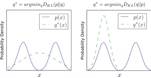
where p(x) is the prior probability, andp(x|y) represents the posterior probability.

Kullback-Leibler Divergence.- If we have two separate probability distributionsP(x) and Q(x) over the same random variable x, we can measure how different these two distributions are using the KLdivergence:

D_KL(P||Q) = E^x∼P

logP(x) Q(x)

applying logarithmic properties, the KLdivergence is defined as follows:

D_KL(P||Q) =E^x∼P[logP(x)−logQ(x)] (2.8) The KL divergence has many useful properties: (1) KL(P||Q) ≥ 0. (2) KL(P||Q) ̸= KL(Q||P). Note that the most notable is that the KL divergence is not negative (see Figure 2.10).

The KL divergence is 0 if and only if P and Q are the same distribution in the case of discrete variables, or equal “almost everywhere” in the case of continuous variables. Because the KL divergence is non-negative and measures the difference between the two distributions, it is often conceptualised as measuring some sort of distance between these distributions. However, it is not a true distance measure because it is not symmetric: DKL(P||Q) ̸= DKL(Q||P) for some P and Q. This asymmetry means that there are important consequences to the choice of whether to useD_KL(P||Q) or D_KL(Q||P).

(46)

Figure 2.10: The KL divergence is asymmetric. Suppose we have a distribution p(x) and wish to approximate it with another distribution q(x). Therefore, we have the choice of minimising either D_KL(p||q) or D_KL(q||p). (Left) The effect of minimising D_KL(p||q). (Right) The effect of minimising D_KL(q||p). Source: Image extracted from (Goodfellow et al., 2016).

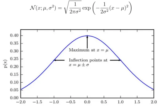
Gaussian Distribution.- The most commonly used distribution over real numbers is the normal distribution, also known as the Gaussian distribution:

N(x;µ, σ²) = r 1

2πσ²exp

− 1

2σ²(x−µ)²

(2.9)

Figure 2.11: The normal distribution (Goodfellow et al., 2016). The normal distribution N(x;µ, σ²) exhibits a classic “bell curve” shape, with the x coordinate of its central peak given by µ, and the width of its peak controlled by σ. In this example, thestandard normal distribution, withµ= 0 andσ = 1.

The two parameters µ ∈ R and σ ∈ (0,∞) control the normal distribution. The parameter µ gives the coordinate of the central peak. This is also the mean of the Master Program in Computer Science - UCSP 23

(47)

2.3. Unsupervised Learning for Anomaly Detection distribution: E[x] = µ. The standard deviation of the distribution is given by σ, and the variance by σ². Figure 2.11 illustrates the normal distribution.

When we evaluate the PDF, we need to square and invert σ. When we need to frequently evaluate the PDF with different parameter values, a more efficient way of parametrizing the distribution is to use a parameterβ ∈(0,∞) to control theprecision or inverse variance of the distribution:

N(x;µ, β⁻¹) = r β

2π exp

−1

2β(x−µ)²

(2.10) Normal distributions are a sensible choice for many applications. In the absence of prior knowledge about what form a distribution over the real numbers should take, the normal distribution would be a good default choice.

2.3.2 Vanilla Autoencoders

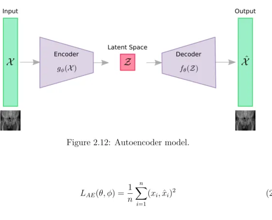
The Vanilla Autoencoder (AE) is a neural network designed to learn an identity function in an unsupervised way to reconstruct the original input while compressing the data in the process in order to discover a more efficient and compressed representation (Hinton and Zemel, 1994; Goodfellow et al., 2016). An autoencoder consists of two networks:

1. Encoder: It translates the original high-dimensional input into the latent space. The latent space is also known as latent low-dimensional code, hidden representation or hidden code. Therefore, the input size is larger than the output size.

2. Decoder: The decoder network recovers the data from the latent space to the original space with a similarly configured transformation.

Figure 2.12 presents an illustration of the autoencoder model. Given X ∈ R^d to be the model input. The encoder functiong(.) parameterized byϕ transformsX into the latent space Z ∈ R^d

′, where d^′ < d. Finally, the decoder function f(.) parameterized byθ reconstructed the input fromZ. Therefore, the reconstructed input is defined as:

Xˆ=f_θ(g_ϕ(X)) (2.11)

The parameters (θ, ϕ) are learned together to output a reconstructed data sample equal to the original input, X ∼ f_θ(g_ϕ(X)). In other words, to learn an identity function.

There are different metrics to minimize the reconstruction error, which is a measure of deviation of ˆX from the original input X, such as cross entropy, or as simple as Mean Squared Error (MSE) loss:

(48)

Figure 2.12: Autoencoder model.

L_AE(θ, ϕ) = 1 n

n

X

i=1

(x_i,xˆ_i)² (2.12)

wherenis the example number,x_i is thei-th example, and ˆx_iis thei-th reconstruction.

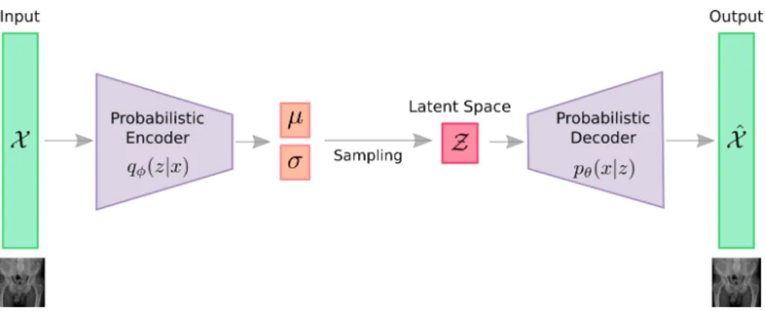
2.3.3 Variational Autoencoders

Variatonal Autoencoder (VAE) can be defined as being an autoencoder whose training is regularised to avoid overfitting and ensure that the latent space has adequate properties that enable a generative process. Just as a standard autoencoder, a VAE is an architecture composed of both an encoder and a decoder, and it is trained to minimize the reconstruction error between the encoded-decoded data and the initial data. However, in order to introduce some regularisation of the latent space, it has a slight modification of the encoding-decoding process: instead of encoding an input as a single point, it encodes the input as a distribution over the latent space (Kingma and Welling, 2014; Rezende et al., 2014).

VAE is deeply rooted in the methods of variational Bayesian inference and graphical model (see Figure 2.13). Given this distribution as p_θ, parameterized by θ. The relationship between the data input X and the latent space vector Z can be fully defined by: (1) priorp_θ(z), (2) likelihood p_θ(x|z), (3) posteriorp_θ(z|x). Assuming that the real parameter θ^∗ for this distribution is known, and in order to generate a sample that looks like a real data point x_i, we follow these steps: First, sample a z_i from a prior distribution p_θ^∗(z). Second, a value x_i is generated from a conditional distributionp_θ^∗(x|z =z_i).

The optimal parameterθ^∗ is the one that maximises the probability of generating Master Program in Computer Science - UCSP 25

(49)

2.3. Unsupervised Learning for Anomaly Detection

Figure 2.13: The graphical model involved in a variational autoencoder. Solid lines denote the generative distributionp_θ(.) and dashed lines denote the distributionq_ϕ(z|x) to approximate the intractable posterior p_θ(z|x).

real data samples:

θ^∗ = arg max

θ n

Y

i=1

p_θ(x_i) (2.13)

Commonly, we use the log probabilities to convert the product into a sum:

θ^∗ = arg max

θ n

X

i=1

logp_θ(x_i) (2.14)

On the other hand, the equation to better demonstrate the data generation process involves the encoding vector:

p_θ(x_i) = Z

p_θ(x_i|z)p_θ(z)dz (2.15)

Unfortunately, it is not easy to computep_θ(x_i) in this way, as it is very expensive to check all the possible values ofz and sum them up. To narrow down the value space to facilitate faster searching, a new approximation function to output is introduced. It is a likely code given an input x, q_ϕ(z|x) parameterized by ϕ. An illustration of VAE is shown in Figure 2.14

Now, the structure looks like an autoencoder:

1. The conditional probability p_θ(x|z) defines a generative model, similar to the decoder f_θ(Z) introduced above. p_θ(x|z) is also known as probabilistic decoder.

2. The approximation functionq_ϕ(z|x) is theprobabilistic encoder, playing a similar role as g_ϕ(X) above.

(50)

Figure 2.14: Illustration of the variational autoencoder architecture.

Loss Function: ELBO The estimated posterior q_ϕ(z|x) should be very close to the real onep_θ(z|x). In this regard, the Kullback-Leibler divergence is used to quantify the distance between these two distributions. KL divergence DKL(X||Y) measures how much information is lost if the distribution Y is used to represent X. In our case, we want to minimize D_KL(q_ϕ(z|x)||p_θ(z|x)) with respect to ϕ. Then, expanding the equation taking into account the preliminary concepts, the KL divergence estimation is defined as follows:

D_KL(q_ϕ(z|x)||p_θ(z|x)) = Z

q_ϕ(z|x) log q_ϕ(z|x) p_θ(z|x)dz

q_ϕ(z|x) log q_ϕ(z|x)p_θ(x) p_θ(z, x) dz

q_ϕ(z|x)

logp_θ(x) + log q_ϕ(z|x) p_θ(z, x)

dz

DKL(qϕ(z|x)||pθ(z|x)) = logpθ(x) + Z

qϕ(z|x) log qϕ(z|x) p_θ(z, x)dz

DKL(qϕ(z|x)||pθ(z|x)) = logpθ(x) + Z

qϕ(z|x) log qϕ(z|x) p_θ(z|x)p_θ(z)dz

D_KL(q_ϕ(z|x)||p_θ(z|x)) = logp_θ(x) +E^z∼qϕ(z|x)

logq_ϕ(z|x)