The suitability of the discrete scheme and associated a priori error estimates for the virtual element solution, as well as for its fully computable projection, are inferred. Furthermore, Strang-type estimates are applied to derive the a priori error estimates for the components of the virtual element solution, as well as for its fully computable projections and postprocessed pressure.
Introduction
To deal with the above nonlinearity, we follow [58] and introduce the velocity gradient as a new unknown. This includes the basic assumptions on the polygon mesh, the definition of the local virtual element space, and the projections and interpolants to be used along with their respective approximation properties.
The continuous problem
The model problem
The continuous formulation
Furthermore, using the Cauchy-Schwarz inequality and estimate (1.16) from (1.15), we conclude that A is Lipschitz-connected with the constant LA := max{1, κ, γ0,α1}, i.e. 1.18) Furthermore, we show below that A is also strongly monotone. Thanks to the Lipschitz continuity and strong monotonicity of the operator A, the proof is a direct application of [97, Theorem 25.B].
The mixed virtual element method
- Preliminaries
- The virtual element space and its approximation properties
- The discrete scheme
- Analysis of the discrete scheme
The Mixed Virtual Elements Method 17 We now introduce the interpolation operator ΠKk :H1(K)→HkK, which is defined for each τ ∈H1(K) as the unique ΠKk(τ)inHkK such that. In what follows we define the mixed virtual element scheme itself for our nonlinear problem (1.12).
The a priori error estimates
Computable approximations of σ, p and u
In this way, we are now able to provide the theoretical rates of convergence for σbh,ph, anduh. In addition, let σbh and (ph,uh) be the discrete approximations shown in (1.48) and (1.50), respectively.
A convergent approximation of σ in the broken H(div)-norm
Numerical results
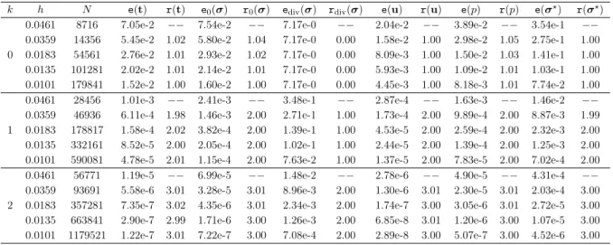
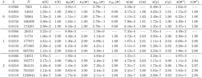
In Tables 1.1 to 1.6 we summarize the convergence history of the augmented mixed virtual element scheme (1.57) as applied to Examples 1 and 2. A fixed-point argument and the Babuška-Brezzi theory are applied there to derive the well-positioned of the resulting continuous formulation.
The Navier-Stokes equations
The model problem
Then, it is not difficult to see that (2.3) and the incompressibility condition div(u) = 0 in Ω, are equivalent to the pair of equations given by. 2.5) We emphasize here that we have eliminated the pressure from the original model (2.1). However, using the second equation in (2.4) we can recover with a post-processing formula in terms of σ and u.
The augmented mixed formulation
In particular, the third equation of (2.6) gives σ =σ0+cI, withσ0∈H0(div; Ω) and constantc given explicitly in terms ofu of. Up to minor changes caused by the present inhomogeneous Dirichlet boundary condition foru , the unique solvability of ( 2.11 ) was fundamentally derived in [ 35 ].
The virtual element subspaces
- Preliminaries
- The virtual element subspace of H 1 (Ω)
- The virtual element subspace of H 0 (div; Ω)
- L 2 -orthogonal projections
The virtual element subspace 42 which is the basis of the subspace of polynomials on K of degree exactly `−1 or. The virtual element subspaces 47 Then, as was noted in section 3.3 of [30], it is easy to see that diameterh.
The discrete forms
The discrete bilinear form A h
In what follows we refer in turn to Rhk,Pkh andPhk, the global counterparts of the projectionsRKk (cf. We end this section by noting that, after reviewing the definition of AKh (cf. 2.47 )), one might suspect the bilinear form SK,∇, which acts as a stabilizer of the term. A similar remark applies to AK,dh (cf. 2.42)) and the probability of multiplying its components AK,d and SK,d by the same constant.
The discrete trilinear form B h
But, as proved by (2.58), the constant that really matters is not the one that results from only a few terms of the whole expression defining Ah, but the definite one that gives the ellipticity of this bilinear form, namely α(Ω), which depends on several other constants and parameters. Nevertheless, this may well become just a theoretical exercise since some of the constants involved may not be explicitly known. On the other hand, the boundedness of the bilinear formBh is established in the following result.
The discrete linear form F h
Discrete forms 58, together with the Cauchy-Schwarz inequality and the fact that Phk(τd) = Phk(τ)d. On the other hand, adding and subtracting Pkh(z), using the Cauchy-Schwarz inequality and applying (2.9) and the estimate (2.40), we find that. Then, applying the Cauchy-Schwarz inequality in (2.59), and then using the limit of Phk, the Cauchy-Schwarz inequality, the limit of ic (cf.
The virtual element scheme
- The solvability analysis
- The a priori error analysis
- Computable approximations of σ, u, and p
- A convergent approximation of σ in the broken H (div; Ω)-norm
In this section we follow the approach from Section 3.2 in [34] and use a fixed-point strategy to analyze the solvability and stability of the Galerkin scheme (2.66). Virtual element scheme 68 Then, according to the second equation in (2.4) and the decomposition of σ given by (2.7) and (2.8), we suggest the following computable pressure approximation:. 2.101) The following lemma defines the corresponding a priori error estimate. It proceeds exactly as the proof of Lemma 5.3 in [31], and therefore we refer to that work and omit the details here.
Numerical Tests
Test 1
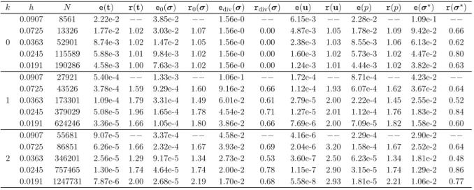
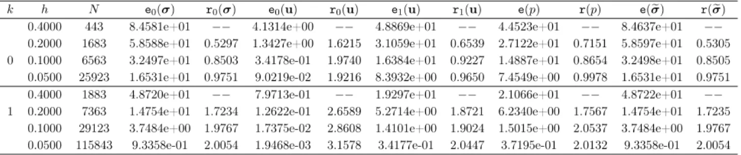
In Tables 2.1 to 2.3 we summarize the convergence history of our extended mixed virtual element scheme for the mesh in Figure 2.1. We also note that the convergence rate O(hk+1) is reached by all the errors, with the exception of ku−ukb 0,Ω, which converges with order k+ 2. Numerical tests 72 that our post-processed voltageσehim may not improve in one -satisfying order provided by the first approximation σbh with respect to the broken H(div) norm.
Test 2
In Tables 2.4 through 2.7, we summarize the convergence history of our extended mixed virtual element scheme. We observe the robustness of our method with respect to different values of the viscosity. In particular, it is interesting to observe that for the first triangular mesh using µ= 0.01 and k= 0, the method was not convergent (at least 50 iterations were used as a limit), in contrast to the results when we use distorted square meshes.

Test 3
Regarding the discrete problem, we have proposed the simultaneous use of virtual element subspaces for H1 and H(div) to approximate the velocity and the pseudovoltage respectively. Discontinuous piecewise polynomial functions of degree ≤k, together with Raviart-Thomas and Lagrange elements of order k+ 1, respectively, are used in [8] to approximate the strain rate, the vorticity, the normal heat flux, the pseudo stress, the velocity , and the temperature of the liquid. In fact, the pseudo stress and the velocity of the fluid are approximated by virtual element subspaces of H(div) and H1, respectively, while a virtual element subspace of H1 is used to approximate the temperature.
The model problem and its continuous formulation
The model problem and its continuous formulation 81, which together with (3.14) gave the H-ellipticity of the bilinear form A+B(z;·,·) for sufficiently small z, that is, for each z∈H1(Ω) such atkzk1,Ω≤ αA. On the other hand, the bounding of the bilinear form A follows (cf. 3.16) Moreover, given φ∈H10(Ω), it follows from the Cauchy-Schwarz inequality and the trace theorems inH(div; Ω) and H1(Ω) that . On the other hand, it follows from (3.9), the properties of the tensor K and the Poincaré inequality, that a is a bounded and H-elliptic bilinear form with the constants kKk∞,Ω and αa, respectively.
The virtual element subspaces
- The virtual subspace of H 1 (Ω)
- The virtual subspace of H 1 (Ω)
- The virtual subspaces of H 0 (div; Ω)
- The global virtual subspaces
- L 2 -orthogonal projections
The virtual element subspaces 84 It is well known that for each ψ∈ QKk the projection RKk (ψ)∈Pk+1(K) is fully computable using only degrees of freedom (3.25) (cf. [4,13]). The virtual element subspaces 85, whose local degrees of freedom, for a given τ ∈HkK, are given by. The virtual element subspaces 86 (APϕh) that existC >0, independently of h, such that for every integer∈[2, k+2] holds.
The discrete forms
In the following, for each k≥0, we denote by Pkh, Phk and PPhk the global counterparts of the projections PkK, PKk and PPKk, respectively, which were presented in section 3.3.5. On the other hand, since the local version aK :QKk × QHk →R is of the bilinear form a(cf. Also, from the first equation (3.49) and the properties of the tensor K, it is easy to see that there exists CK>0, depending only on K, so that 3.51) We can now introduce the locally discrete bilinear form aKh :QKk × QKk →R, which is defined by.
The virtual element scheme and its stability analysis
A priori error estimates
On the other hand, collecting and subtracting Phk+1(u), using the Cauchy-Schwarz and Holder inequalities, Lemma3.6 and the compact injection (3.13), we find that. Further, by adding and subtracting the appropriate terms, summing over all K∈ Th, and then taking the supremum over ψh ∈ Qhk, we derive the estimate (3.86) depending only on Kandc1. Also, collecting and subtracting suitable terms, we find that. 3.95) Moreover, using the limit of Bh (cf.
A convergent approximation of σ in the broken H (div; Ω)-norm
Numerical Examples
Introduction 109 The purpose of this chapter is to present the basic tools for developing post-failure analysis for mixed VEM. As usual in the VEM approach, we introduce fully computable approximations for the virtual approximation of the flow variable and establish its corresponding a priori error estimates. Upper bounds are shown for the scalar variable in the L2 norm, the VEM flux variable in the H(div) norm, its projection in the L2 norm, and postprocessing in the broken H(div) norm.
The model problem
The virtual element method
Virtual subspace and its approximation properties
Discrete formulation
To this end, we first note that the bilinear form b (cf. (4.5)) can be explicitly computed for all. In particular, to define SK, we can consider the bilinear form associated with the identity matrix in RnKk with respect to the local basis determined by degrees of freedom (4.10), and whereKk = dimHhK. The following two lemmas determine the properties of the bilinear formaKh and the consistency error between aKh and aK, respectively.
Computable approximations
Virtual subspace and its approximation properties 114 According to definition (4.14), the global discrete bilinear form ah :Hh×Hh → R can be defined by summing the local contribution (4.14), i.e. Furthermore, we have the following result on a priori error estimates for schemes (4.4) and (4.18). The result is a consequence of [28, Theorem 6.1] and the direct use of the approximation properties provided by (4.6) and Lemma 4.3.
A posteriori error analysis
- Preliminaries
- A posteriori error estimator
- Upper bound
- Lower bound
For this purpose, in the following we assume that the limit Γ is such that ΓN lies in a convex part of Ω. Assume that Ω is a connected field and that ΓN lies on the boundary of a convex part of Ω, that is, there exists a convex domain B such that Ω⊂ B and ΓN ⊆∂B. The upper bounds of the terms depending on the network parameter K and it will be derived next.
Numerical Tests
Test 1. Smooth solution: behaviour of the estimator under uniform refinement 127
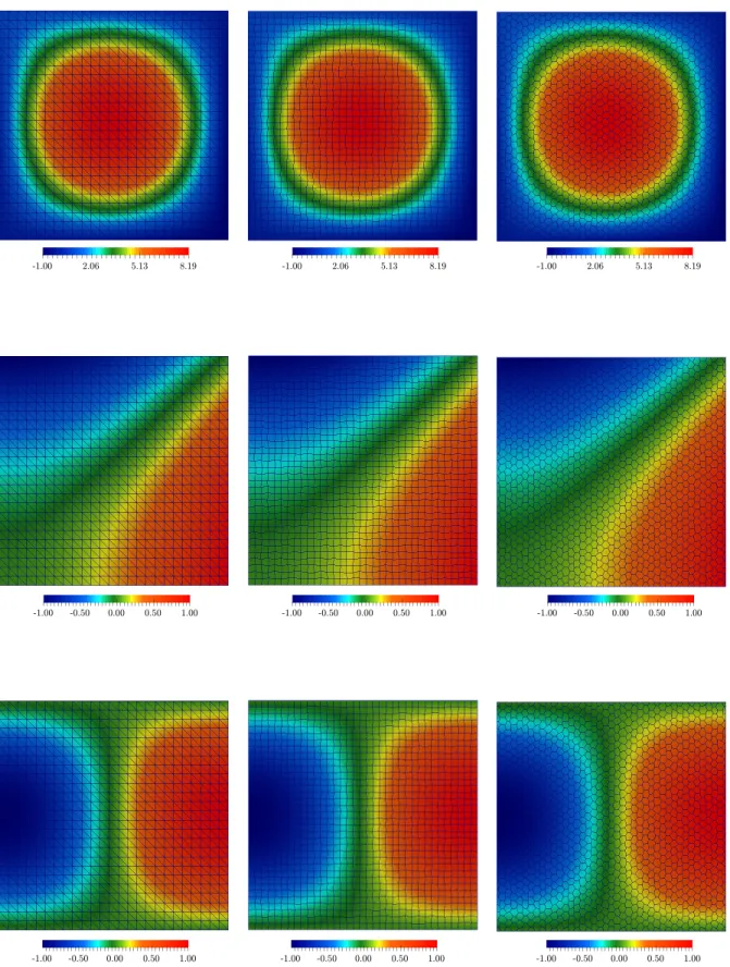
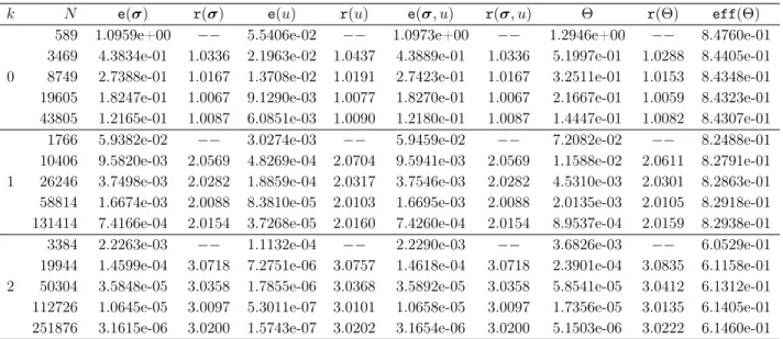
Table 4.1 shows the error convergence history for each variable and estimator on a sequence of uniformly refined hexagonal grids, showing that both converge to the optimal rate for the polynomial ratesk= 0,1,2. Furthermore, we see from Table 4.2 that each term of the error estimator converges to an optimal order k+ 1. Both such lines are outside Ω, but we expect regions of high gradients near the left boundary.
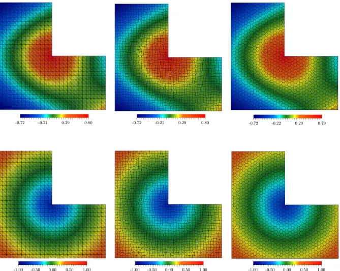
Test 3. L-shaped domain solution: adaptive refinement
This is clearly shown in Table 4.3, where the convergence rates of the global error and the estimator at each step of the adaptive algorithm are listed along with the performance index. Behavior of global error and estimator in adaptive refinement of hexagonal grids (cf. Figure 4.3). Convergence history of estimator components in adaptive refinement of hexagonal meshes (see Figure 4.3 below).

The nonlinear Brinkman model
The model problem and its continuous formulation
From the fourth and last equation (5.7), note that t and σ must belong to L2tr(Ω) (cf. Moreover, the analysis of the continuous formulation (5.9) is based on the results of the nonlinear analysis (cf. [68, Section 2.2] In this way, the regularity variational formulation (5.9) determined by the following theorem.
The mixed virtual element method
The Nonlinear Brinkman Model 140 We now introduce the interpolation operator ΠKk : H1(K) → HkK, which is defined for each τ ∈ H1(K) as the uniqueΠKk(τ)inHkK such that. Find (th,σh)∈Xkh×Hkh such that. 5.26) The inconsistency between A and Ah is established by the following result. Then there exists a unique (th,σh) ∈Xkh×Hkh solution of (5.26) and there exists a positive constant C, independent of h, such that.
A posteriori error analysis
Reliability
Then, using Id = 0, div(I) = 0, and the fact that hIν,gi = 0 (which is a consequence of the compatibility condition for the Dirichlet data g discussed in Section 5.2.1), we obtain. Furthermore, by similar arguments to the proof of Lemma 5.4 in [58, Section 5] (see also [40, Lemma 5.9]), together with Lemma 5.9, and the fact that the number of elements in ωe is bounded, the term|R(curl( ϕ−ϕh))|is bounded accordingly. Then, as a consequence of Lemmas 5.8 and 5.10, the triangle inequality and the lower bound in (5.24), we conclude that there exists C >0, independent of h, such that.
Efficiency
It follows from bounding the moduli of the two expressions on the right-hand side of (5.49). Next, the upper limits of the terms which depend on the mesh parameters hK and he will be derived below. To this end, we make use of the results and estimates proved in [40, Section 5.4], whose proofs use techniques based on bubble functions, expansion operators, and discrete tracking and inverse inequalities.
Numerical results
Example 1
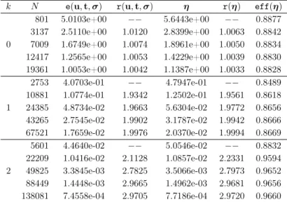
The purpose of this test is to verify the asymptotic behavior of the estimator with a smooth solution and under uniform refinements. Tables 5.1 to 5.3 show the convergence history of the errors and the estimator on the three order of uniformly refined meshes, indicating that all converge at the optimal rate for polynomial degrees k= 0,1,2. Convergence history of some terms using a uniformly generated series of meshes consisting of distorted squares.
Example 2
Example 3
Manzini, A posteriori residual error estimation for the virtual element method for elliptic problems, ESAIM Math. Gatica, A Mixed Virtual Element Method for the Pseudotension Velocity Formulation of the Stokes Problem, IMA J. Tierra, An Augmented Mixed Finite Element Method for the Navier-Stokes Equations with Variable Viscosity, SIAM J.

Example 1, history of convergence using triangles
Example 1, history of convergence using quadrilaterals
Example 1, history of convergence using hexagons
Example 2, history of convergence using triangles
Example 2, history of convergence using quadrilaterals
Example 2, history of convergence using hexagons
Example 3, history of convergence using triangles
Example 3, history of convergence using quadrilaterals
Example 3, history of convergence using hexagons
Test 1, history of convergence using triangular meshes
Test 1, history of convergence using distorted squares meshes
Test 1, history of convergence using hexagonal meshes
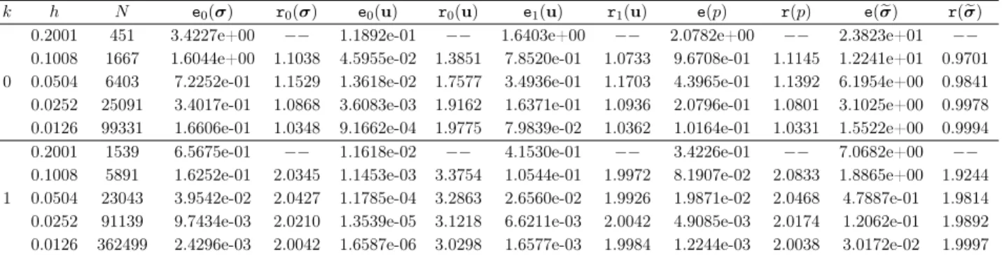
Test 2, history of convergence using triangular meshes (k = 0)
Test 2, history of convergence using triangular meshes (k = 1)
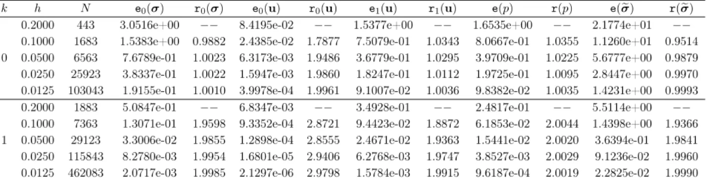
Test 2, history of convergence using distorted squares (k = 0)
Test 2, history of convergence using distorted squares (k = 1)
Example 1: Convergence history using distorted squares with k = 0
Example 2: Convergence history using triangles with k = 0