Computer Science and Artificial Intelligence Laboratory Technical Report
MIT-CSAIL-TR-2012-018 June 29, 2012
Integrated Robot Task and Motion Planning in the Now
Leslie Pack Kaelbling and Tomas Lozano-Perez
Integrated robot task and motion planning in the now
Leslie Pack Kaelbling and Tom´as Lozano-P´erez CSAIL, MIT, Cambridge, MA 02139
{lpk, tlp}@csail.mit.edu
Abstract
This paper provides an approach to integrating geometric motion planning with logical task planning for long-horizon tasks in domains with many objects. We propose a tight integration between the logical and geometric aspects of planning. We use a logical representation which includes entities that refer to poses, grasps, paths and regions, without the need for a priori discretization. Given this representation and some simple mechanisms for geometric inference, we characterize the pre-conditions and effects of robot actions in terms of these logical entities.
We then reason about the interaction of the geometric and non-geometric aspects of our domains using the general-purpose mechanism of goal regression (also known as pre-image backchaining).
We propose an aggressive mechanism for temporal hierarchical decomposition, which postpones the pre-conditions of actions to create an abstraction hierarchy that both limits the lengths of plans that need to be generated and limits the set of objects relevant to each plan.
We describe an implementation of this planning method and demonstrate it in a simulated kitchen environment in which it solves problems that require approximately 100 individual pick or place operations for moving multiple objects in a complex domain.
1 Introduction
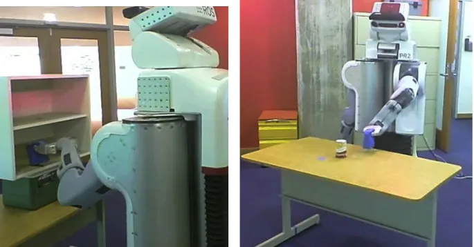
Robots act to achieve goals in the world: moving the paint sprayer to paint a car, opening a door to let someone in, moving the plates to empty the dishwasher, and so on. Consider a robot operating in a relatively simple home environment: there are a few rooms, some food items in the kitchen refrigerator, dishes and pans on the shelves, some tables and counter surfaces, a stove with two burners (in red) and a sink (in blue). A simulation of such an environment is shown in figure 1. The robot has the goal of serving food items on the kitchen table and then tidying up. Even ignoring the intricate manipulation required to open jars, cut food, actually cook the items or clean the dishes, achieving these simple goals requires a long sequence of actions: bringing the food items to the preparation area, getting the pans, bringing the food to the pan, cooking the items, serving them on plates and then cleaning up (putting everything back in the refrigerator, washing the pans and even picking up the dirty cup someone left in the living room). As part of this process, the robot must perform actions that were not explicitly mentioned in the goals; for example, moving items out of the refrigerator to reach the desired food items and then replacing them. Throughout, the robot must choose how to grasp the objects, where to stand so as to pick up and put down objects, where to place the objects in the regions, what paths to use for each motion, and so on.
The question we address in this paper is: How should we structure the computational process that controls the robot so that it can effectively achieve its goals?
1
Figure 1: Simulated apartment environment with pans, cups, sink, stove, and furniture.
We propose a strategy for combining symbolic and geometric planning, first introduced by Kael- bling and Lozano-P´erez [2011a], that enables the solution of very large mobile manipulation prob- lems. It sacrifices optimality as well as the ability to solve some highly intricate problems in order to be able to address many problem instances that are too large to solve by other means presently available. The solution concept could be applied to many other large domains, but here we focus on, and tailor the system to, the problem of mobile manipulation.
One strategy for designing such goal-achieving robots is to engineer, compute offline or learn a
2
Figure 2: PR2 robot manipulating objects
policythat directly encodes a mapping from world states or beliefs over world states into actions that ultimately achieve the goals. Such policies can vary in complexity, from a fixed sequence of actions independent of the world state, to a feedback loop based on one or more sensed values, to a complex state-machine. Although they can be derived from the engineer’s knowledge of the world dynamics and the goals, they would not explicitly represent or reason over the goals or world states.
This approach is critical for domains with significant time pressure and can be very successful for tasks with limited scope, such as spray painting cars and vacuuming carpets or controlling the robot while cutting vegetables. However, we expect that, for sufficiently complex tasks such as building a complete robot household assistant, where the action sequences have intricate dependencies on the initial state of the world, on extrinsic events, and on the outcomes of the robot’s actions, explicitly represented policies would need to be intractably large.
We pursue an alternative approach to designing robots for complex domains in which the robot chooses its actions based on explicit reasoning over goals and representations of world states. Note that the goals and states must refer to aspects of the world beyond the robot itself, for example, to the people in the household or the food in the refrigerator. Classical artificial intelligence planning [Ghallab et al., 2004] (often known in robotics as task planning) provides a paradigm for reasoning about fairly general goals and states to derive sequences of “abstract” actions. However, we must ultimately choose particular low-level robot motions, and classical task planning methods are not able to address the geometric and kinematic challenges of robot motion planning in high- dimensional continuous spaces.
The original conception, in Shakey [Nilsson, 1984], of the interaction between a task planner and a motion planner was that the task planner would construct “high-level” plans based on some weak geometric information (such as connectivity between rooms) and the steps of these plans would be achieved in the world by “intermediate-level” primitives, which would involve perception and
3
motion planning, and ultimately issue “low-level” controls. This conception has generally proved unworkable; in particular, a much tighter integration between task planning, geometric planning and execution is generally necessary [Cambon et al., 2009]. The need for tight integration of levels is even more pronounced in the presence of uncertainty and failure [Haigh and Veloso, 1998, Burgard et al., 1998]. An especially challenging case is when “high-level” actions may be motivated primarily by the need to acquire information about object placements.
It is clear that non-geometric goals affect geometric goals: for example, we need to properly place the pan on the stove to cook the food. But the converse is also true: the geometry can affect the structure of the non-geometric plan. For example, when planning to put away objects given some possible containers, the size and locations of the containers affect which object(s) can be placed in which containers. Therefore, we need an approach to planning that allows the non-geometric and geometric considerations to interact closely.
This paper describes a hierarchical approach to integrating task and motion planning that can scale to robot tasks requiring long sequences of actions in domains involving many objects, such as the one in figure 1. However, both task and motion planning are computationally intractable problems; we cannot hope to solve hard puzzles efficiently. Our method exploits structural decom- positions to give large improvements in computation time, in general, at some cost in suboptimality of execution, but without compromising completeness in many domains.
There is substantial uncertainty in any real mobile manipulation problem, such as the PR2 robot, shown in figure 2, that matches our simulated robot. This uncertainty stems both from the typical sources of sensor and motion error, but also from fundamental occlusions and uncertainties:
how is the robot to know what is in a particular kitchen drawer? Handling uncertainty is a critical problem. In this paper, we establish a planning and execution framework that will serve as a foundation for an approach that deals with deeper issues in non-determinism and partial observability [Kaelbling and Lozano-P´erez, 2011b, 2012].
1.1 Approach
The most successful robot motion planning methods to date have been based on searching from an initial geometric configuration using a sample-based method that is either bidirectional or guided toward the goal configuration. As the dimensionality of the problem increases (due to multiple movable objects) and the time horizon increases (due to the number of primitive actions that must be taken) direct search in the configuration space becomes very difficult. Ultimately, it cannot scale to problems of the size we are contemplating, nor does it provide a method for integrating non-geometric goals and constraints into the problem.
We propose a hierarchical approach to solving long-horizon problems, which performs a temporal decomposition by planning operations at multiple levels of abstraction. By performing a hierarchical decomposition, we can ensure that the problems to be addressed by the planner always have a reasonably short horizon, making planning feasible.
In order to plan with abstract operators, we must be able to characterize their preconditions and effects at various levels of abstraction. For reasons described above, even at abstract levels, geometric properties of the domain may be critical for planning; but if we plan using abstracted models of the operations, we will not be able to determine a detailed geometric configuration that results from performing an operation. To support our hierarchical planning strategy we, instead, plan backwards from the goal using the process known as goal regression[Ghallab et al., 2004] in task planning andpre-image backchainingin motion planning [Lozano-P´erez et al., 1984]. Starting
4
from the set of states that satisfies the goal condition, we work backward, constructing descriptions of pre-images of the goal under various abstract operations. The pre-image is the set of states such that, if the operation were executed, a goal state would result. The key observation is that, whereas the description of the detailed world state is an enormously complicated structure, the descriptions of the goal set, and of pre-images of the goal set, are often describable as simple conjunctions of a few logical requirements.
In a continuous space, pre-images might be characterized geometrically: if the goal is a circle of locations inx, y space, then the operation of moving one meter in x will have a pre-image that is also a circle of locations, but with thex coordinate displaced by a meter. In a logical, or combined logical and geometric space, the definition of pre-image is the same, but computing pre-images will require a combination of logical and geometric reasoning. We support abstract geometric reasoning by constructing and referring to salient geometric objects in the logical representation used by the planner. So, for example, we can say that a region of space must be clear of obstacles before an object can be placed in its goal location, without specifying a particular geometric arrangement of the obstacles in the domain. This approach allows a tight interplay between geometric and non-geometric aspects of the domain.
The complexity of planning depends both on the horizon and the branching factor. We use hierarchy to reduce the horizon, but the branching factor, in general, remains infinite: there are innumerable places to put an object, innumerable paths for the robot to follow from one configura- tion to another, and so on. We introduce the notion ofgeneratorsthat make use both of constraints from the goal and heuristic information from the starting state to make choices from these infinite domains that are likely to be successful; our approach can be extended to support sample-based backtracking over these choices if they fail. Because the value-generation process can depend on the goal and the initial state, the values are much more likely to be successful than ones chosen through an arbitrary sampling or discretization process.
Even when planning with a deterministic model of the effects of actions, we must acknowledge that there may be errors in execution. Such errors may render the successful execution of a very long sequence of actions highly unlikely. For this reason, we interleave planning with execution, so that all planning problems have short horizons and start from a current, known initial state. If an action has an unexpected effect, a new plan can be constructed at not too great a cost, and execution resumed. We refer to this overall approach ashpnfor “hierarchical planning in the now.”
In the rest of this section, we provide a more detailed overview of thehpn approach. We use a simple, one-dimensional environment to illustrate the key points.
1.1.1 Representing objects, relations and actions
Figure 3 shows three configurations of an environment in which there are two blocks, aand b, on a table. They are each 0.5 units wide, and their position is described by the (continuous) position of their left edges. The black line in the figure represents the table and the boxes beneath the line represent regions of one-dimensional space that are relevant to the planning process. The configuration space, then, consists of points inR2, with one dimension representing the left edge of aand the other representing the left edge ofb. However, some (la, lb) pairs represent configurations in which the blocks are in collision, so the free configuration space is R2 with the illegal locus of points{(la, lb)|la−lb<0.5}, which is a stripe along the diagonal, removed.
At the lowest level of abstraction, the domain is represented in complete detail, including shapes and locations of all objects and the full configuration of the robot. This representation is used to
5
a b goal
swept(a)
swept(b)
a b
goal
swept(a)
swept(b)
a b
goal
swept(a)
swept(b) Place(a, aLoc)
Place(b, bLoc)
aLoc bLoc
aLoc bLoc
aLoc bLoc
Figure 3: Simple one-dimensional environment: starting configuration, intermediate configuration after movingbout of the way, final configuration witha in the goal region.
support detailed motion planning.
At higher levels of abstraction, we use logical representations to characterize both geometric and non-geometric aspects of the world state. To describe our example domain, we use instances of the following logical assertions:
• In(o, r) indicates that object ois completely inside the region r;
• ObjLoc(o, l) indicates that the left edge of object o is at locationl; and,
• ClearX(r, x) indicates that no objects overlap regionr, except possibly for objects named in the set x.
Note that by “logical” representations, we mean representations that are made up of explicit references to entities in the domain (including objects, regions, paths, and poses), relations among these entities (including object in region, or pose near object) that have truth values in a given state, and Boolean combinations of these relations. We emphatically do not mean that these representations are free of numbers, as the examples above attest. The key benefit of logical representations is that they give us compact representations of large, possibly infinite, sets of world states and of the dynamic effects of actions on such large or infinite domains. Our key requirement on the representations will be that, given a logical description, we must be able to determine
6
whether a geometric world state satisfies that description. For example, we must be able to test whether In(A,goal) is true of a world state.
To complete a domain representation, we must also describe the available actions. We will use operators which are loosely modeled on the operators of classical task planning. An operator describes the preconditionsof an action and its effects. In our simple environment, we have three types of operators, each of which has as its effect one of the types of assertions mentioned above.
The first one actually causes a physical effect in the environment; the other two are essentially inference rules that reduce one logical condition to another.
• Place(o, ltarget) places objectoat a target locationltarget; the effect isObjLoc(o, ltarget). The preconditions are that the object be in some location,lstart, before the operation takes place and that the region “swept” by the object moving from lstart toltarget be clear except for o, that is,ClearX(sweptVol(o, lstart, ltarget),{o}).
• In(o, r): the effect isIn(o, r) ifObjLoc(o, l) is true for some location, such that the volume of objecto when located atl is contained in region r.
• Clear(r, x): the effect isClearX(r, x) if all objects in the universe except those in the set x do not overlap regionr; that is, that for all objectsonot inx,In(o,r), where ¯¯ r is the spatial complement ofr (that is, the spatial domain minus r).
1.1.2 Regression and generators
Inhpn, the goal of the system is to reach some element in a set of states of the world, described using a logical expression. So, for example, a goal might be for object ato be in the region goal, which would be writtenIn(a,goal). The planning algorithm proceeds by applying a formal description of the operations in the domain to find one that might achieve the goal condition, then adopting the preconditions of that operation as a new sub-goal. This process of goal-regression proceeds until all of the conditions in the subgoal are true in the current world state.
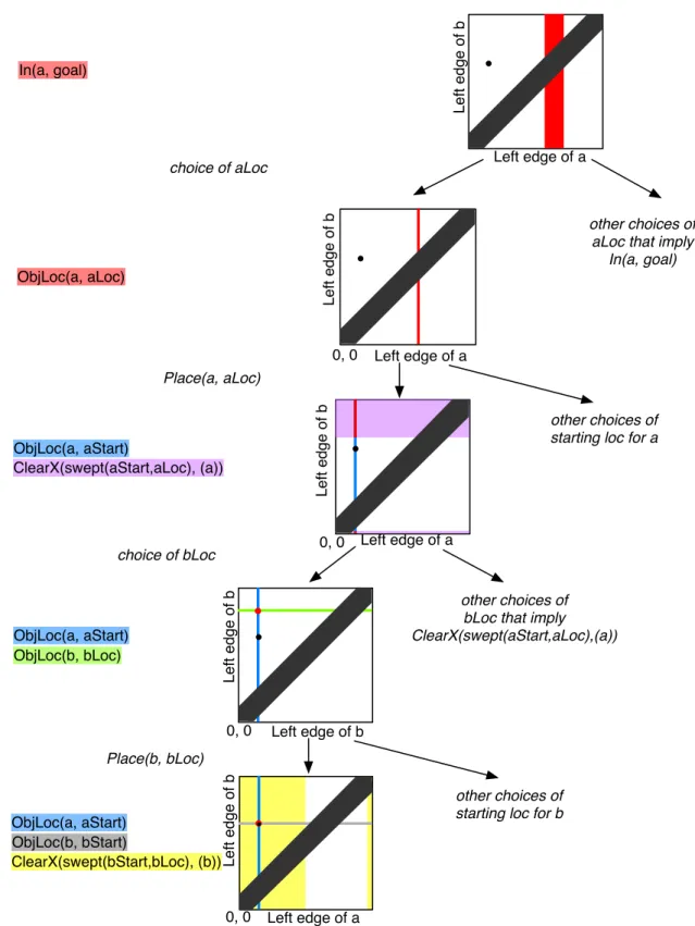
To illustrate regression and generation inhpn, we work through a very simple example in detail.
The goal of our simple planning problem is for blockato be in the goal region, which is indicated in orange. There is no explicit robot in this environment: to keep the space low-dimensional, we will simply consider motions of the objects along the one-dimensional table.
Figure 4 shows a path in the regression search tree through sets of configurations of the blocks.
Recall that the configuration space in this domain is the positions of the left edges of the two blocks, which isR2, minus the configurations along the diagonal in which the objects would be in collision with one another.
• The root of the tree is the starting state of the regression search. It is the goal condition In(a,goal). That logical condition corresponds to a region of configuration space illustrated in red. The goal does not specify the location ofb, so it can have any legal value; but the left edge ofais constrained to lie in an interval that will guarantee that the entire volume ofais in the goal region. For reference in all of the configuration-space pictures in this figure, the starting state, which is a specific position of both boxes, is shown as a black dot.
• The first choice in the search process is to choose a location for a that will cause it to be contained in the goal region. A generator will construct or sample possible locations for a;
we illustrate a specific choiceaLoc, shown in figure 3 as a short vertical blue line. The logical 7
Left edge of a
Left edge of b
Left edge of a
Left edge of b
0, 0
Left edge of a
Left edge of b
0, 0
Left edge of b
Left edge of b
0, 0
Left edge of a
Left edge of b
0, 0 In(a, goal)
ObjLoc(a, aLoc)
choice of aLoc
ObjLoc(a, aStart)
ClearX(swept(aStart,aLoc), (a))
ObjLoc(a, aStart)
ObjLoc(a, aStart) ObjLoc(b, bLoc)
ObjLoc(b, bStart)
ClearX(swept(bStart,bLoc), (b))
other choices of aLoc that imply
In(a, goal)
Place(a, aLoc)
Place(b, bLoc)
other choices of bLoc that imply ClearX(swept(aStart,aLoc),(a)) choice of bLoc
other choices of starting loc for a
other choices of starting loc for b
Figure 4: A path through the regression search tree in configuration space for the simple one dimensional environment.
8
goal In(a,goal) is reduced to ObjLoc(a,aLoc). This is not the entire pre-image of the goal, and for completeness it might be necessary to backtrack and search over different choices.
• The next step in the search is to compute the pre-image ofObjLoc(a,aLoc) under the action Place(a,aLoc). In order for that action to be successful, it must be thatais located at some initial location. The Place operator allows the starting location of the object to be chosen from among a set of options including that object’s location in the initial state, as well as other salient locations in the domain. In this example, we choose to move it from its location in the initial state,aStart; to enable that move, we must guarantee that the region of space through whichamoves as it goes fromaStart toaLoc is clear of other objects. The requirement that a be located at aStart corresponds to the vertical blue locus of points in the configuration space. The requirement that the swept volume be clear turns into a constraint on the location of b. If the left edge of b is in one of the intervals shown in purple, then it will be out of the way of movinga. The pre-image is the conjunction of these two conditions, which is the intersection of the blue and purple regions in the configuration-space figure, which is shown in red.
• The current configuration of the objects (black dot) is not in the goal region, so the search continues. We search for a placement of object b that will cause it to satisfy the ClearX constraint, suggesting multiple positions includingbLoc. This leads to the configuration-space picture in which the green line corresponds to object b being at location bLoc. Intersected with the constraint, in blue, that a be at location aLoc, this yields the subgoal of being in the configuration indicated by the red dot.
• Finally, the operatorPlace(b,bLoc) can be used to move objectb, subject to the preconditions thatb be located at bStart (shown as the gray stripe) and that the swept volume forb from bStart tobLoc be clear except for objectb. The clear condition is a constraint on objectato be in the yellow region. The intersection of all these conditions is a point which is equal to the starting configuration, and so the search terminates. (Note that, in general, the pre-image will not shrink to a single point, and the search will terminate when the starting state is contained in a pre-image).
The result of this process is a plan, read from the leaf to the root of the tree, to move object b to locationbLoc and then move objectato locationaLoc, thereby achieving the goal.
1.1.3 Hierarchy
Viewed as motion planning problems, the tasks that we are interested in solving have very high dimensionality, since there are many movable objects, and long planning horizons, since the number of primitive actions (such as linear displacements) required for a solution is very large. They are alsomulti-modal[Sim´eon et al., 2004, Hauser and Ng-Thow-Hing, 2011, Barry et al., 2012] requiring choosing grasps and finding locations to place objects, as well as finding collision-free paths. As such, they are well beyond the state of the art in motion planning.
Viewed as task-planning problems, the tasks that we are interested in solving require plans with lengths in the hundreds of actions (such as pick, place, move, cook). The combination of long horizon, high forward branching factor, and expensive checking of geometric conditions means that these problems are beyond the state of the art for classic domain-independent task-planning systems.
9
Our approach will be to use hierarchy to reduce both the horizon and the dimensionality of the problems.
• We reduce the horizon with a temporal hierarchy in terms of abstract actions, which comprise the process of achieving conditions to enable a primitive action as well as the primitive action itself. The lowest layer of actions are hand-built primitive actions, and the upper layers are constructed dynamically by a process of postponing pre-conditions of actions.
• The hierarchy also reduces dimensionality of sub-problems because fewer objects and fewer properties of those objects are relevant to sub-problems; the factored nature of the logical representation, which allows us to mention only those aspects of state that are relevant, naturally and automatically selects a space to work in that has the smallest dimensionality that expresses the necessary distinctions.
We have developed a hierarchical interleaved planning and execution architecture. In hpn, a top-level plan is made using an abstract model of the robot’s capabilities, in which the “primitive”
actions correspond to the execution of somewhat less abstract plans. The first subgoal in the abstract plan is then planned for in a less abstract model, and so on, until an actual primitive action is reached. Primitive actions are executed, then the next pending subgoal is planned for and executed, and so on. This process results in a depth-first traversal of a planning and execution tree, in which detailed planning for future subgoals is not completed until earlier parts of the plan have both been constructed and executed. It is this last property that we refer to as “in the now.”
This mechanism results in a natural divide-and-conquer approach with the potential for sub- stantially decreasing complexity of the planning problem, and handles unexpected effects of ex- ecution through monitoring and replanning in a localized and efficient way. On the other hand, a consequence of decomposition is that highly coupled problem instances will generally not be handled efficiently (but, there is no method that can handle all problems efficiently). We believe this trade-off is worth making since we expect that highly coupled problems are relatively rare in common-place activities. It also requires care and insight to construct a hierarchical domain spec- ification that works effectively with hpn. We hope that such domain descriptions can eventually be constructed automatically, but experience with some hand-built hierarchies is a pre-requisite to developing an automatic approach.
1.2 Related work
There is a great deal of work related to our approach, in both the robotics and the artificial intel- ligence planning literatures. We discuss a small part of the related work in robotics manipulation planning, in hierarchical AI planning, and work that seeks to integrate these two approaches.
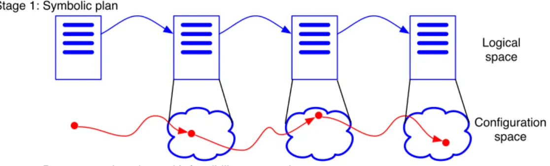
1.2.1 Integrating logical and geometric planning
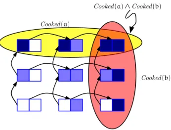
The need for integrating geometric and task planning has long been recognized [Nilsson, 1984, Kambhampati et al., 1991, Malcolm, 1995]. It is a difficult problem, requiring integration or coor- dination between planning processes in two very different spaces: the space of logical representations and the space of points in a geometric configuration space. Figure 5 gives a schematic illustration of some strategies for performing this integration, including thehpn approach. In these figures, there is a logical state description, represented as a conjunction of logical assertions, and a geometric
10
Logical space
Configuration space Stage 2: Per-step motion plans with feasibility assumed
Stage 1: Symbolic plan
(a) Shakey [Nilsson, 1984]: logical phase followed by geometric phase.
Logical space
Configuration space Detailed symbolic representation
(b) Dornhege et al. [2009]: geometric configuration encoded in logical state.
Planning in joint symbolic and configuration space
Symbolic space
Configuration space
(c) ASyMov [Cambon et al., 2009]: search in product of logical and configuration spaces.
Stage 1: Symbolic plan with new symbols for cspace constraints
Stage 2: Path planning in the now with feasibility between constrained regions guaranteed Symbolic space, with
geometric entities
Configuration space
(d) HPN: Backward search in logical space, dynamically incorporating geometric constraints.
Figure 5: Schematic illustration of different methods for combining logical and geometric planning.
In each case, the logical space is illustrated as a list of logical assertions (blue or purple lines), red dots represent points in the complete geometric configuration space of the problem, blue or purple clouds represent subsets of configuration space that are consistent with the associated logical state, and red arrows represent geometric paths through configuration space.
11
state description, represented as poses of all movable objects and the robot. In our schematics, the logical state is shown as a “document”, with horizontal blue lines representing logical assertions as
“sentences” in the document. Each logical state corresponds to a subset of the space of possible configurations of the objects and robot. In the figures, that subset is shown as a blue “cloud” in configuration space; individual configurations are red dots within the cloud. A blue arc between logical states indicates that the transition between those states is allowable according to the logical domain dynamics. A red arc between geometric configurations indicates that there is a collision-free path that respects the geometric and dynamic constraints of the objects and robot between those two configurations.
The simplest approach, taken in the Shakey project [Nilsson, 1984] and illustrated in figure 5(a), is to plan in two stages. The environment is represented logically at a high level of abstraction (for example, characterizing which objects are in which rooms or whether an object is blocking a door) and in the first stage an abstract plan is constructed using that representation. It is assumed that robot motion plans can be constructed that will implement the abstract actions in the logical plan:
those are constructed step-by-step in a second stage, as the high-level plan is executed.
A risk of this approach is that the high-level actions will not, in fact, be executable. Dornhege et al. [2009] extend this approach by adding the ability to use general computational procedures to evaluate the symbolic predicates and to compute the effects of taking actions. They represent a detailed geometric state (including the robot pose) in the logical state and run a motion-planning algorithm to validate proposed logical actions, so that at the end of the planning process they have a complete, valid, geometric plan. One drawback of this approach is that choices for geometric variables, such as grasps and object placements, need to be discretized in advance and there is a very large forward branching factor.
Instead of having the logical search be prior to the geometric search or to contain it, we may instead think of the search as proceeding in a product space of logical and geometric spaces, representing both discrete properties of the state and the poses of objects and the robot. This approach was pioneered by Cambon et al. [2009] in the ASyMov system, and is illustrated in figure 5(c). This system performs a forward search in the product space, using purely logical plans as a heuristic for searching in the product space. At the geometric level, a sample-based planner is used to find a low-level motion plan that “threads” through the geometric images of a sequence of logical states that satisfy logical transition constraints and ultimately terminates in a goal region.
The search in ASyMov is made more efficient by first testing feasibility of geometric transitions in roadmaps that do not contain all movable obstacles, and then doing a complete verification of candidate solutions. Significant attention is paid to managing the search process, because the sample-based geometric planning methods never fail conclusively, making it critical to manage the allocation of time to different motion-planning problems well. Plaku and Hager [2010] extend this approach to handle robots with differential constraints and provide a utility-driven search strategy.
The hpnapproach, illustrated in figure 5(d) is neither driven by a static logical representation of the environment nor carried out simultaneously in the geometric and logical spaces. It can be thought of as dynamically constructing new logical entities that represent geometric constraints such that the existence of a logical plan guarantees the existence of a geometric plan. It proceeds in two stages. The first stage takes place at the logical level, proceeding backward from the goal, which projects into a set of geometric configurations. Generally speaking, the pre-image of a logical action will require the creation of new entities, in order for its geometric aspects to be described logically. For example, if the last action is to place an object in some region of space, we may need
12
to create entities representing the object’s pose and the volume of space that must be clear in order to place the object. Logical sentences that represent these new geometric entities and constraints are shown in purple in the logical states of the figure (they are purple, because they combine blue logical representation with red geometric representation). The determination of pre-images requires geometric computation, but does not commit to a particular path through configuration space. Thus, after the first logical planning stage, we have a sequence of “subgoals” described logically and shown as purple projections into configuration space. In the second stage, during execution, any motion planner can be called to find a path from the current configuration to any configuration in the next purple cloud.
In contrast to the methods described thus far, which usegenerativeplanning methods to synthe- size novel action sequences from declarative descriptions of the effects of actions, Wolfe et al. [2010]
use ahierarchical task networkhtn[Nau et al., 2003] approach, in which a kind of non-deterministic program for achieving the task is specified. Logical representations are used at the high levels, but the primitive actions are general-purpose programs combining perception and geometric planning.
The focus of the algorithm is on finding the cost-optimal sequence of actions that is consistent with the constraints specified by the htn. Significant efficiency is gained by focusing only on relevant state variables when planning at the leaves. It is difficult to compare the htn approach directly to the generative planning approaches: it generally requires more knowledge to be supplied by the authors of the domain description; however, the ability to supply that control knowledge may make some problems tractable that would not be solvable otherwise.
Haigh and Veloso [1998] describe the design ofRogue, an architecture for integrating symbolic task planning, robot execution and learning. The task planner inRogueis the Prodigy4.0 planning and learning system [Fink and Veloso, 1996]. Prodigy, likehpn, uses backward chaining to construct sequences of goal-achieving plan steps; it also uses forward simulation of plan steps to update its (simulated) current state. Roguebuilds on this approach, interleaving planning and execution on the real robot. The system executes a step on the robot when Prodigy selects a plan step to simulate.
This is similar tohpn’s approach to planning and executing “in the now”, althoughRoguedid not use hierarchical planning. Nourbakhsh [1998] also describes a hierarchical approach to interleaving planning and execution that is similar to ours, but which does not integrate geometric reasoning.
Keller et al. [2010] outline a planning and execution system that is in spirit very similar to ours, using the planning method described by Dornhege et al. [2009]. Uncertainty is handled with online execution monitoring and replanning, including the ability to postpone making plans until sufficient information is available. Beetz et al. [2010] outline an ambitious system for downloading abstract task instructions from the web and using common-sense knowledge to expand them into detailed plans ultimately executable on a mobile manipulator. In the context of that project, Kresse and Beetz [2012] specify a system that combines logical reasoning with rich force-control primitives: the high-level planner specifies constraints on motions and the low-level planner exploits the null space of those constraints to find feasible detailed control policies for the robot.
1.2.2 Manipulation planning with multiple objects
Most work on manipulation planning focuses on interacting with a single object, and is often restricted to path planning for a fixed target configuration or to grasp selection. A few early systems, like Handey [Lozano-P´erez et al., 1987], and more recent systems, like HERB [Srinivasa et al., 2009] and OpenRave [Diankov, 2010], integrate perception, grasp and motion planning, and control. Sim´eon et al. [2004] present a general decomposition method for manipulation planning
13
that allows complex plans involving multiple regrasp operations.
Planning among movable obstacles generalizes manipulation planning to situations in which additional obstacles must be moved out of the way in order for a manipulation or motion goal to be achieved. In this area, the work of Stilman and Kuffner [2006] and Stilman et al. [2007] allows solution of difficult manipulation problems that require objects to be moved to enable motions of the robot and other objects. This method takes an approach very similar to ours, in that it plans backwards from the final goal and uses swept volumes to determine, recursively, which additional objects must be moved and to constrain the system from placing other objects into those volumes. It does not, however, offer a way to integrate non-geometric state features or goals into the system or allow plans that move an object more than once. van den Berg et al. [2008]
develop a probabilistically complete approach to this class of problems, but it requires explicit computation of robot configuration spaces and so it is limited to problems with few degrees of motion freedom.
Work by Dogar and Srinivasa [2011] augments pick-and-place with other manipulation modal- ities, including push-grasping, which significantly improve robustness in cluttered and uncertain situations. Planning in hybrid spaces, combining discrete mode switching with continuous geome- try, can be used to sequence robot motions involving different contact states or dynamics. Hauser and Latombe [2010] have taken this approach to constructing climbing robots. Recently, Hauser and Ng-Thow-Hing [2011] have formulated a very broad class of related problems, including those with modes selected from a continuous set, as multi-modal planning problems and offer a general sample-based approach to them.
There are other approaches to multi-level treatment of the robot-motion planning problem.
Zacharias and Borst [2011] introduce the capability map, which characterizes the difficulty of a motion planning problem in advance of solving it, based on the number of orientations from which a position can be reached. Such a capability map can be used, top-down, to help generate feasible planning problems at more concrete levels of abstraction. Stulp et al. [2012] learn to characterize places from which different types of actions can be executed effectively. Westphal et al. [2011]
interweave reasoning about qualitative spatial relationships with sample-based robot motion plan- ning. A qualitative plan is made using highly approximate models of objects and the robot gripper;
this qualitative plan is used to guide sampling in the motion planner with a considerable gain in efficiency. Plaku et al. [2010] address robot motion planning with dynamics using a hybrid discrete- continuous approach that uses high-level plans in a discrete decomposition of the space to guide sample-based planning.
1.2.3 Hierarchical and factored planning
Hierarchical approaches to planning have been proposed since the earliest work of Sacerdoti [1974], whoseABSTRIPSmethod generated a hierarchy by postponing preconditions. Hierarchical plan- ning techniques were refined and analyzed in more detail by Knoblock [1994] and Bacchus and Yang [1993] among others. These approaches may require backtracking across sub-problems, and it has also been shown that abstractions can slow planning exponentially [B¨ackstr¨om and Jonsson, 1995].
The Fast Downward system of Helmert [2006] and its descendants are some of the most efficient current logical planners: their strategy is to convert the environment into a non-binary representa- tion that reveals the hierarchical dependencies more effectively, then exploit the hierarchical causal structure of a problem to solve efficiently.
Work onfactored planninggeneralizes the notion of hierarchical planning, and seeks to avoid the 14
costly backtracking through abstractions of previous approaches. In factored planning, the problem is divided into a tree of sub-problems, which is then solved bottom-up by computing the entire set of feasible condition-effect pairs (or sometimes more complex relations) for that subproblem, and passing that result up to the parent. This approach was pioneered by Amir and Engelhardt [2003]
and advanced by others, including Brafman and Domshlak [2006] and Fabre et al. [2010].
Marthi et al. [2007, 2008] give mathematical semantics to hierarchical domain descriptions based on angelic non-determinism, and derive a planning algorithm that can dramatically speed up the search for optimal plans based on upper and lower bounds on the value of refinements of abstract operators. They also give conditions under which plan steps may be executed before planning is complete without endangering plan correctness or completeness. Goldman [2009] gives an alternative semantics that incorporates angelic non-determinism during planning and adversarial non-determinism during execution.
The angelic-semantics methods are more directed than the factored-planning approaches: they use top-down information to focus computations at the lower levels, but require the decomposition to be done by hand. Mehta et al. [2009] pursue a related approach, but automatically learn a decomposition, in domains with a strict serializability property. Subgoals serialize if there is an ordering of them such that one may be achieved first and then maintained true during the achievement of the other.
Our approach differs from these in that it neither backtracks through abstractions during plan- ning, nor computes sets of solutions, nor assumes strong serializability. It makes top-down commit- ments to subgoals that are such that, if the subgoals do serialize, then the planning and execution are both efficient. If the decomposition assumptions fail, but the environment is such that no actions are irreversible, the system will eventually achieve the goal by falling back to planning in the primitive model. The result is that problems that are decomposable can be solved efficiently;
otherwise, the system reverts to a non-hierarchical approach.
1.3 Outline
The rest of the paper is organized as follows. Section 2 introduces the representations and algorithms we use for planning in discrete and continuous domains. It uses as a running example a highly simplified one-dimensional “kitchen” environment: this domain combines logic and geometry in interesting and subtle ways, but is sufficiently simple that it can be presented and understood in its entirety. Section 3 introduces thehpn recursive planning and execution architecture, explains our flexible approach to hierarchical planning, and illustrates these ideas in the one-dimensional kitchen environment. Section 4 describes the formalization, in hpn, of a large-scale mobile manipulation environment with a Willow Garage PR2 robot as well as results of tests and experiments. In section 5 we describe the strengths and limitations of the system and articulate directions for future work. Throughout the paper, many of the detailed definitions and examples are postponed to appendices; it is safe to delay reading them until more detail is desired.
2 Representation and planning
Fluentsare logical assertions used to represent aspects of the state of the external physical world that may change over time; conjunctions of fluents describe sets of world states, and are used to to specify goals and to represent pre-images. In a finite domain, it is possible to describe a world state
15
completely by specifying the truth values of all possible fluents. In continuous geometric domains, it is not generally possible to specify the truth values of all possible fluents; but fluents remain useful as a method for compactly describing infinite sets of world states.
We represent goals and subgoals as conjunctions of fluents that characterize subsets of the underlying state space, including both geometric and non-geometrical properties, and represent the current state of the world using a typical non-logical world model that describes positions, orientations and shapes of objects and the configuration of the robot, as well as other properties such as whether plates are clean or food is cooked.
We begin this section by introducing an extension of our simple planning environment, which we use to motivate and make concrete the descriptions in the following sections. We then describe the geometric representation of world states and the logical representation of goals. The logical representation forms the basis for describing the operations in the environment. We show how to extend a standard operator-description formalism to handle our infinite domain, and present the regression planning algorithm in detail.
2.1 One-dimensional kitchen environment
So that we can build intuition and provide completely detailed examples during the narrative of this section, we will work with a highly simplified one-dimensional kitchen environment. In this environment:
• Objects have finite extent along a line. They can be moved along the line but cannot pass through each other.
• The robot operates like a crane, in the sense that it is above the line and need not worry about collision with the objects.
• A segment of the line is defined to be asink region where objects can be washed.
• A segment of the line is defined to be astove region where objects can be cooked.
• Objects must be washed before they can be cooked.
• The goal is to have several objects be cooked.
Figure 6 shows a plan and execution sequence for the goal of cooking a single object. In section 4 we extend this environment to operate in three spatial dimensions, with a real robot model and a large number of both permanent (not movable) and movable objects.
2.2 World states
Aworld stateis a completely detailed description of both the geometric and non-geometric aspects of a situation. World states can be represented in any way that is convenient. We never attempt to represent a complete characterization of the world state in terms of fluents. The only requirement is that, for each fluent type, there is a procedure that will take a list of arguments and return the value of that fluent in the world state.
In the one-dimensional kitchen environment, the world state is a dictionary mapping the names of objects to a structure with attributes for location, size, whether or not they are clean and whether or not they are cooked. In this structure,s[o].loc represents the location of objecto in world state
16
Figure 6: Plan for cooking objecta(magenta). It requires moving objectsb(orange) andc (cyan) out of the way first, then putting a in the sink, washing it, putting a on the stove, and finally cooking it. When an object is clean, it becomes green; when it is cooked, it becomes brown. The red region is thestove and the blue region the sink; the leftmost object is a.
17
s. We also uses[o].minand s[o].max to name the left and right edges of the object (loc is the same asmin).
2.3 Fluents
A fluent is a condition that can change over time, expressed as a logical predicate applied to a list of arguments, which may be constants or variables. We use these logical expressions to specify conditions on geometric configurations of the robot and the objects in the world, as well as other non-geometric properties, such as whether something is clean or cooked. The meaning of a fluent f is defined by specifying a test,
τf :args, s→ {true,false} ,
where args are the arguments of the fluent, s is a world state and the value of the test is either true orfalse.
Agroundfluent (all of whose arguments are constants) then represents the subset of all possible world states in which the associated test is true. A conjunction of fluents represents a set of world states that is the intersection of the world state sets represented by the elements of the conjunction;
this is the same as the set of world states in which the tests of allof the fluents evaluate to true.
The fluents we use to describe the one-dimensional kitchen domain, together with their tests, are the following:
• ObjLoc(o, l): the left edge of object ois at (real-valued) position l, τObjLoc((o, l), s) :=|s[o].loc−l|< δ .
whereδ is a small value used throughout this implementation to make the numerical opera- tions robust.
• In(o, r): object ois entirely contained in regionr,
τIn((o, r), s) := (r.min≤s[o].min+δ) & (r.max ≥s[o].max −δ) .
• ClearX(r, x): region r is clear, except for exceptions, x, which is a set of objects, τClearX((r, x), s) :=∀o6∈x. s[o]∩r=∅ .
• Clean(o): object o is clean,
τClean((o), s) := (s[o].clean=True) .
• Cooked(o): object ois cooked,
τCooked((o), s) := (s[o].cooked =True) .
A goal for our planning and execution system is a conjunction of ground fluents describing a set of world states. The goal of having objectabe clean and objectbbe cooked can be articulated
as: Clean(a) &Cooked(b) .
During the course of regression-based planning, intermediate goals are represented as conjunctions of fluents as well. We will write s∈ G to mean that world state s is contained in the set of goal statesG.
18
2.4 Operator descriptions
We describe the dynamics of the environment (that is, the effects of the robot’s actions on the state of the world) using operator descriptions. They are based on ideas fromstrips[Fikes and Nilsson, 1971] andpddl[McDermott, 2000], but are extended to work effectively in continuous domains as described in section 2.5 and to form a hierarchy in section 3. Rather than defining a traditional formal language for describing operators, our implementation makes use of procedures to compute the preconditions of an operation. Each operator description has the following components:
• variables: Names occurring in the effectfluents and chooseclauses. An operator descrip- tion is actually aschema, standing for concrete operator descriptions for all possible bindings of the variables to entities in the domain.
• effect: A list of fluents with variables as arguments, characterizing the effects that this operator can be used to achieve.
• precondition: A list of fluents that describe the conditions under which, if the operator is executed, the effect fluents will be guaranteed to hold.
• primitive: An actual primitive operation that the robot can execute in the world.
• choose: A list of variable names and, for each, a set of possible values it can take on.
The semantics of an operator description is that, if the primitive action is executed in any world statesin which all of the precondition fluents hold, then the resulting world state will be the same ass, except that any fluent specified as an effect will have the value specified in the resulting state.
The formalization of the dynamics of the one-dimensional kitchen environment in terms of op- erator descriptions illustrates the use of operator descriptions and provides a completely concrete description of the planning domain. Each operator description takes the state of the world at plan- ning time,snow, and the goal to which it is being applied during goal regression, γ, as arguments.
We explain the roles ofsnow andγ when we discuss generators in section 4.1.4.
• An object can be washed if it is in the sink.
Wash((o), snow, γ):
effect: Clean(o) pre: In(o,sink)
• An object can be cooked if it is clean and on the stove.
Cook((o), snow, γ):
effect: Cooked(o) pre: In(o,stove)
Clean(o)
• An object can be moved to a target location if there is an unoccluded path for it. The PickPlace(o, ltarget) operator moves object o to target location ltarget. It has a choose variable,lstart, which is thesource locationfrom which the object is being moved tolt. These
19
values are provided bygenerators, which are discussed further in section 2.5.3. The location of the object in the plan-time state,snow[o].loc, is a reasonable starting location, as are extreme valid positions within each of the important regions of the domain.
For each generated value of lstart, there is a instantiation of this operator, which has as its preconditions that object obe located at lstart and that the volume of space thato is swept through as it moves fromlstart toltarget be clear of all objects except foro. We usewarehouse here to refer to some region of space that is “out of the way” that might be use as a temporary storage place for objects.
PickPlace((o, ltarget), snow, γ):
effect: ObjLoc(o, ltarget)
choose: lstart ∈ {snow[o].loc} ∪generateLocsInRegions((o,{warehouse,stove,sink}), snow, γ) pre: ObjLoc(o, ls)
ClearX(sweptVol(o, ls, lt),{o})
In this simple one-dimensional world, the swept “volume” is simply an interval comprising the volume of the object at the start and target locations and the volume between them:
sweptVol(o, ls, lt) = [min(ls, lt),max(ls, lt) +o.size]
The remaining two operators are used to achieve the ClearX and In fluents. They are defini- tional in the sense that they are not associated with a primitive action: they serve as a kind of inference rule during the planning process, removing the effect fluent from the goal and replacing it with a set of “precondition” fluents.
• The conditions for placing an object into a region reduce to the placement of the object at an appropriate target location, that will cause the object to be contained in the region.
In((o, r), snow, γ):
effect: In(o, r)
choose: l∈generateLocsInRegion((o, r), snow, γ) pre: ObjLoc(o, l)
• To specify that region r must be clear except for the set x of “exception” objects that are allowed to overlap the region, we rewrite the condition positively, saying that all objects not in the setx must be completely contained in the region of space that is the complement ofr;
that is, they are in the set U \r, where U is the spatial universe of the domain and \ is the set difference operator.
Clear((r, x), snow, γ):
effect: ClearX(r, x)
pre: In(o, U \r) foro∈(allObjects\x)
20
2.5 Extending operator descriptions to continuous domains
In order to adequately formalize operation in continuous domains, we have made several extensions to the typical planning formalisms for discrete domains. These include extending the notion of a primitive action, allowing for limited forms of logical reasoning, and handling variables with infinite domains.
2.5.1 Primitives
Actions that are primitive from the perspective of task planning can themselves be very complex, in terms of computation, sensing, and actuation. For example, if pick is a primitive operation, specifying an object and a grasp for that object, it might require the robot to visually sense the object’s location, call a motion planner to generate a path to a pre-grasp pose, execute that trajectory, and finally execute a robust grasping subroutine that uses tactile information to close in on the object appropriately.
2.5.2 Limited logical reasoning
In the originalstrips formulation of planning, all arguments of all fluents were discrete and each stripsrule stated all positive and negative effects of each action; reasoning about the effects of ac- tions was then limited to set operations on the fluent sets characterizing the subgoals, preconditions, and effects of operators.
In hpn, fluents may have continuous values or values drawn from very large discrete sets as arguments, making it typically impossible to enumerate every fluent that becomes true or false as a result of taking an action. To account for this, we must perform some limited logical reasoning.
We do this by providing a method for each fluent that takes another fluent and determines whether the first fluent entails the second fluent and a method that takes another fluent and determines whether the first fluent contradictsthe second fluent.
A fluentf1entails fluentf2 if and only if the set of states in whichf1holds is a (possibly proper) subsetof the set of states in whichf2 holds. A fluent f1 contradicts fluentf2 if the set of states in which f1 holds has an empty intersection with the set of states in which f2 holds.
Sometimes the effect of an operator on a state (and, therefore, its regression) is more subtle than simply contradicting or entailing another fluent. For instance, the regression of the condition of havingxdollars under the action of spendingydollars is havingx+ydollars. We additionally allow the specification of aregression method for each operator description that takes a fluent as input and returns another fluent that represents the regression of the first fluent under the operation. The entailment, contradiction, and regression methods for the one-dimensional kitchen environment are described in detail in appendix A.
2.5.3 Generators
Most operations can be achieved in multiple ways: a robot can move along multiple paths, an object can be picked up from many starting locations, two objects may be fastened together with one of many different bolts. When an operator description has a clause of the form
choose v∈D ,
21
it means that there is a possible instantiation of the operator for each possible binding of variable v to a value in the set D.
In very large or continuous environments, however, it is infeasible to consider all possible bind- ings; in such cases, we may take advantage of special-purpose procedures that can take into account both the state of the world at planning time,snow, and the subgoal being planned for,γ, and gen- erate bindings for v that are likely to be successful in that context. The subgoal γ is used to avoid generating bindings that would result in operator preconditions that directly contradict γ. The current statesnow is used for heuristic purposes, to generate bindings for which the operator preconditions are relatively cheap to achieve in the current state:
choosev∈generator(args, snow, γ) .
In our current implementation, generators just return a short list of possible bindings; it would be possible to extend the software architecture so that they are generators in the computer-science sense, which can be called again and again to get new values, to support backtracking search. In such an approach, with appropriate sampling methods, it may be possible to guarantee resolution completeness. However, we believe it will be most effective to emphasize learning to generate a small number of useful values, based in the current state and the goal.
For the one-dimensional kitchen environment, we have a single generator. The procedure generateLocsInRegion((o, r), snow, γ)
takes an object o, a target region r, planning-time state snow and a goal γ, and returns a list of possible locationsl of objectosuch that if owere placed at l,
• owould be contained in region r,
• owould not be in collision with any object that has a placement specified in goal γ, and
• owould not overlap any region required to be clear in goalγ.
It is preferred but not required that this location be clear insnow: however, if necessary an occluding object in that location can be moved out of the way.
There are, generally, a continuum of such locations. This procedure returns the extreme points of each continuous range of legal locations:
generateLocsInRegion((o, r), snow, γ):
C ={r0 |ClearX(r0, x)∈γ &o6∈x}
O ={vol(o0, l)|ObjLoc(o0, l)∈γ}
R0 =r\(C∪O) return S
{ρ∈R0|f(o,ρ)}{min(ρ),max(ρ)−o.size}
wherevol(o, l) is defined to be the volume of space taken up by objectoif it is placed at locationl.
It begins by finding the set Cof all the regionsr0 that are required to be clear in the goal γ and for whichois not in the set of exceptions; then it finds the setO of all regions that are required to be occupied by placed objects in the goal γ; then R0 is defined to be the set of contiguous regions that result from subtractingC and O from r. Finally, it constructs and returns a set of locations, by finding all of the regionsρinRin whichofits,f(o, ρ), and computing the leftmost and rightmost placements ofoinρ. Testing whether an object fits in a region is trivial in one-dimension: it is just necessary to compare the sizes. This procedure is straightforwardly modified to handle the case when r is in fact a non-contiguous region (represented as a set of contiguous regions).
22
2.6 Regression planning
The regression planning algorithm is an A∗ search through the space of conjunctions of fluents, which represent sets of world states. It takes as arguments the planning-time world statesnow, the goal γ, and the abstraction level α, which is irrelevant for now but which we will discuss in detail in section 3. Pseudo-code for the goal-regression algorithm is provided in appendix B.1.
• Thestarting stateof the search is the planning goalγ, represented as a conjunction of fluents;
• Thegoal testof the search is a procedure that takes a subgoalsg and determines whether all of the fluents are true in the current world statesnow.
• The successors of a subgoal sg are determined by the procedure applicableOps. This procedure determines which instances of the operators are applicable tosg, and performs the regression operation to determine the pre-images ofsg under each of those operator instances.
It is described in detail in appendix B.1.
• Theheuristicdistance from the current statesnow to a subgoalsg is the number of fluents in sg that are not true in snow.
It returns a list, ((−, g0),(ω1, g1), ...,(ωn, gn)) where the ωi are operator instances,gn=γ,gi is the pre-image ofgi+1 underωi, andsnow ∈g0. The pre-imagegi is the set of world states such that if the world is in some stategi and actionωi+1 is executed, then the next world state will be ingi+1. In the current implementation, all operators are assumed to have cost 1; it is straightforward to extend the algorithm to handle different costs for different operators or operator instances. The heuristic we use here is not admissible: it is possible for a single action to make multiple fluents true. We expect that learning a heuristic that is both tighter and closer to admissible will also be an important future research question.
An example result of applying the regression planning algorithm to the one-dimensional kitchen environment is shown in figure 6. The plan, shown in the tree on the left, has 11 steps: gray nodes indicate definitional actions that have no primitive associated with them and green nodes indicate primitive actions. By moving objectb(the orange object) to the right, it clears the region necessary to move objectc(the cyan object) to the right as well. This makes room to moveato the washer.
Objecta is then washed, moved to the stove, and then cooked. This process is shown pictorially, with the initial configuration at the top of the figure, and subsequent world states shown below the primitive action that generated them.
Even this simple example illustrates the interplay between the geometric and the logical plan- ning: geometric details affect which objects must be moved and in what order and logical goals affect the locations in which objects must be placed.
Thus far, our planning process has operated at only two levels: a completely geometric primitive level and a logical task level. This approach can only solve moderately small problems, but it will serve as the basis for the hierarchical extensions described in the next section.
3 Hierarchy and planning in the now
In this section, we provide a method for planning and execution with a multi-level hierarchical decomposition, illustrate a method for constructing such hierarchical decompositions, and demon-
23
strate these methods by handling large problem instances in the one-dimensional kitchen environ- ment.
3.1 hpn architecture
The hpn process is invoked by hpn(snow, γ, α,world), where snow is a description of the state of world when the planner is called;γ is the goal, which describes a set of world states;αis a structure that controls the abstraction level, which we discuss in more detail in section 3.2.4; andworld is an actual robot or a simulator on which primitive actions can be executed. In the prototype system described in this paper,world is actually a geometric motion planner coupled with a simulated or physical robot.
hpn calls the regression-based plan procedure, which returns a whole plan at the specified level of abstraction, ((−, g0),(ω1, g1), ...,(ωn, gn)). The pre-images, gi, will serve as the goals for the planning problems at the next level down in the hierarchy.
hpn(snow, γ, α,world):
p=plan(snow, γ, α) for (ωi, gi)in p
if isPrim(ωi)
world.execute(ωi,snow)
elsehpn(snow,gi,nextLevel(α,ωi),world)
hpn starts by making a plan p to achieve the top-level goal. Then, it executes the plan steps, starting with actionω1, side-effectingsnow so that the resulting state will be available when control is returned to the calling instance of hpn. If an action is a primitive, then it is executed in the world, which causessnow to be changed; if not, then hpnis called recursively, with a more concrete abstraction level for that step. hpn assumes that the fluents used to describe goals are the same at every abstraction level; that is, there is no state abstraction, only operator abstraction. The procedurenextLeveltakes a level of abstractionα and an operatorω, and returns a new level of abstractionβ that is more concrete than α.
Note that the abstract action ωi does not directly affect the planning at the more concrete level; only the subgoal gi is relevant. This means that hpn does not refine plans, in the sense of simply adding details to an existing plan; the plan at a more concrete level may not have any connection to the abstract action at the level above. Also note that hpn does not backtrack across abstraction levels; that is, it commits to the subgoals generated by planning at each level of abstraction. We discuss the consequences of this structure in more detail in section 3.2.3. If the hierarchical decomposition is well chosen, thehpn approach may result in a potentially enormous computational savings; if it is not, then the system may execute useless or retrograde actions.
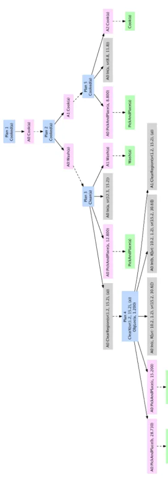
Figure 7 shows a hierarchical version of the plan in figure 6. Blue nodes are goals for planning problems; pink nodes are operations associated with a concrete action; gray nodes are definitional operations. Operation nodes are prefixed withAnwherenis an integer representing the abstraction value at which that operator is being applied.
Instead of one large problem with an 11-step plan, we now have 5 planning problems, with solutions of length 1, 2, 3, 4, and 5. Because planning time is generally exponential in the length of the plan, the reduction in length of the longest plan is significant.
24
Figure 7: Hierarchical planning and execution trees for cooking objecta. This is a solution to the same problem as the flat plan shown in figure 6.25