Computer Science and Artificial Intelligence Laboratory Technical Report
MIT-CSAIL-TR-2015-028 September 21, 2015
Network Maximal Correlation
Soheil Feizi, Ali Makhdoumi, Ken Duffy, Manolis
Kellis, and Muriel Medard
Network Maximal Correlation
Soheil Feizi1,3, Ali Makhdoumi1,3, Ken Duffy2, Manolis Kellis1 and Muriel M´edard1 September 2015
Abstract
Identifying nonlinear relationships in large datasets is a daunting task particularly when the form of the nonlinearity is unknown. Here, we introduce Network Maximal Correlation (NMC) as a fundamental measure to capture nonlinear associations in networks without the knowledge of underlying nonlinearity shapes. NMC infers, possibly nonlinear, transformations of variables with zero means and unit variances by maximizing total nonlinear correlation over the underlying network. For the case of having two variables, NMC is equivalent to the standard Maximal Correlation. We characterize a solution of the NMC optimization using geometric properties of Hilbert spaces for both discrete and jointly Gaussian variables. For discrete random variables, we show that the NMC optimization is an instance of the Maximum Correlation Problem and provide necessary conditions for its global optimal solution. Moreover, we propose an efficient algorithm based on Alternating Conditional Expectation (ACE) which converges to a local NMC optimum. For this algorithm, we provide guidelines for choosing appropriate starting points to jump out of local maximizers. We also propose a distributed algorithm to compute a 1- approximation of the NMC value for large and dense graphs using graph partitioning.
For jointly Gaussian variables, under some conditions, we show that the NMC optimization can be simplified to a Max-Cut problem, where we provide conditions under which an NMC solution can be computed exactly. Under some general conditions, we show that NMC can infer the underlying graphical model for functions of latent jointly Gaussian variables. These functions are unknown, bijective, and can be nonlinear. This result broadens the family of continuous distributions whose graphical models can be characterized efficiently. We illustrate the robustness of NMC in real world applications by showing its continuity with respect to small perturbations of joint distributions. We also show that sample NMC (NMC computed using empirical distributions) converges exponentially fast to the true NMC value. Finally, we apply NMC to different cancer datasets including breast, kidney and liver cancers, and show that NMC infers gene modules that are significantly associated with survival times of individuals while they are not detected using linear association measures.
1 Introduction
Identifying relationships among variables in large datasets is an increasingly important task in sys- tems biology [1], social sciences [2], finance [3], etc. While correlation-based measures capture linear associations, they can fail to infer true nonlinear relationships among variables, which can often occur in real-world applications [4]. One family of measures to infer nonlinear associations among
1 Massachusetts Institute of Technology (MIT), Cambridge, US.
2 Hamilton Institute, Maynooth University, Ireland.
3 These authors contributed equally to this work.
variables is based on mutual information [5,6]. Although mutual information computes a measure of association strength among variables, it does not provide functions through which variables are related to each other. Moreover, reliable computation of mutual information requires an excessive number of samples, particularly for large number of variables [7].
A classical measure to infer a nonlinear relationship between two variables isMaximal Correlation (MC), introduced by Gebelein [8] and studied in references [9–12]. MC infers, possibly nonlinear, transformations of two variables with zero means and unit variances by maximizing their pairwise correlation. MC can be computed efficiently for both discrete [13] and continuous [14] random variables. For discrete variables, under some mild conditions, MC is equal to the second largest singular value of a normalized joint probability distribution matrix [13]. In that case, transfor- mations of variables can be characterized using right and left singular vectors of the normalized probability distribution matrix. Recently, MC has been used in different applications in information theory [15–17], information-theoretic security and privacy [18–20], and data processing [21,22].
Many modern applications include large number of variables with possibly nonlinear relationships among them. Using MC to capture pairwise associations can cause significant over-fitting issues because each variable can be assigned to multiple nonlinear relations. Here we propose Network Maximal Correlation (NMC) as a fundamental measure to capture nonlinear associations in net- works without the knowledge of underlying nonlinearity shapes. In the NMC optimization, each variable is assigned to at most one transformation function with zero mean and unit variance.
NMC infers optimal transformations of variables by maximizing their inner products over edges of the underlying graph. For the case of two variables, NMC is equivalent to MC. The NMC defi- nition does not assume a specific relationship among node variables and the graph structure. For illustration, we consider this relationship in different NMC applications such as graphical model inference. Furthermore, the NMC optimization can be regularized to have even fewer nonlinear transformations to avoid over-fitting issues.
In this paper, we characterize a solution of the NMC optimization using geometric properties of Hilbert spaces for both discrete and continuous jointly Gaussian variables. For discrete random variables, we show that the NMC optimization is an instance of the Maximum Correlation Problem (MCP) which is NP-hard [23–26]. In this case, using results of the Multivariate Eigenvector Prob- lem (MEP) [23], we provide necessary conditions for a global NMC optimum. We also propose an efficient algorithm based on Alternating Conditional Expectation (ACE) [13], which converges to a local NMC optimum. We also provide guidelines for choosing appropriate starting points of the algorithm to jump out of local maximizers. The proposed ACE algorithm does not require forming joint distribution matrices which could be expensive for variables with large alphabet sizes. We also propose a distributed version of the ACE algorithm to compute a 1- approximation of the NMC value for large and dense graphs using graph partitioning.
For jointly Gaussian variables, we use projections over Hermitte-Chebychev polynomials to char- acterize an optimal solution of the NMC optimization. Under some conditions, we show that the NMC optimization is equivalent to the Max-Cut problem, which is NP-complete [27]. However, there exist algorithms to approximate its solution using Semidefinte Programming (SDP) within an approximation factor of 0.87856 [28]. In this case, we provide conditions under which an NMC solution can be computed exactly. Using these results, under some general conditions we show that NMC can infer the underlying graphical model for functions of latent jointly Gaussian variables.
These functions are unknown, bijective, and can be nonlinear. This result broadens the family of continuous distributions whose graphical models can be characterized efficiently.
In real-world applications, often only noisy samples of joint distributions are available. For this case, we prove a finite sample generalization bound, and error guarantees for NMC. In particular, under general conditions we prove that NMC is continuous with respect to joint probability dis- tributions. That is, a small perturbation in the distribution results in a small change in the NMC value. Moreover, we show that Sample NMC (i.e., NMC computed using empirical distributions) converges exponentially fast to the NMC value as the sample size grows.
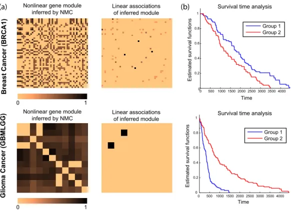
Moreover, we use the NMC optimization to characterize a nonlinear global relevance graph with a certain complexity [29] and propose a greedy algorithm to infer such a nonlinear relevance graph approximately. Finally, we apply NMC to different cancer datasets [30] including breast, kidney and liver cancers and show that using the NMC network, we can infer gene modules that are significantly associated with survival times of individuals while they are not detected using linear association measures.
2 Maximal Correlation
In this section, we introduce notations and review prior work on maximal correlation.
2.1 Notation
SupposeX1 andX2 are two random variables defined on probability space(Ω,F, P) taking values in (X1,B1) and (X2,B2), respectively. The map Xi ∶ (Ω,F) → (Xi,Bi) generates the subalgebra Fi = Xi−1(Bi) of F. Let PXi be the restriction of the measure P on Fi, i = 1,2. For discrete variables,X1 andX2 are their finite support sets with cardinalities∣Xi∣, fori=1,2.
2.2 Definition and General Properties
A Pearson’s linear correlation coefficient between real-valued variables X1 and X2 is defined as cor(X1, X2) = E[(X√1−E[X1]) (X2−E[X2])]
var(X1) √
var(X2) ,
where var(Xi) represents the variance of random variable Xi, for i=1,2. Correlation-based mea- sures capture linear associations between variables, ignoring possible nonlinear relationships.
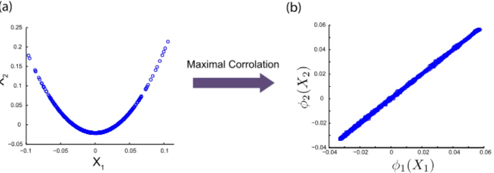
Example 1 SupposeX1is a Gaussian variable with zero mean and unit variance. LetX2=X12. In this case, even though variables are strongly associated with each other, the correlation coefficient between them is close to zero (see e.g. Figure 1-a). It is because these variables are related through a nonlinear transformation. One way to capture such a nonlinear relationship between these variables is to quantify maximum correlation between their, possibly nonlinear, transformations.
In this example, suppose φ1(X1) =α11X12+α12 and φ2(X2) =α21X2+α22, where coefficients αij are selected so that φi(Xi) has zero mean and unit variance, for both i =1,2. In this case, the correlation coefficient between transformed variables is one (see e.g. Figure1-b), capturing a strong nonlinear association between variablesX1 and X2.
Maximal correlation (MC) between variables X1 and X2 which was introduced by Gebelein [8]
captures a nonlinear association between them by selecting, possibly nonlinear, transformation functions φ1(X1) and φ2(X2) so thatφ1(X1) and φ1(X1) have the highest correlation among all other transformation functions with zero means and unit variances.
−0.1 −0.05 0 0.05 0.1
−0.05 0 0.05
0.1 0.15 0.2 0.25
X1 X2
−0.04 −0.02 0 0.02 0.04 0.06
−0.04
−0.02 0 0.02 0.04 0.06
Maximal Corrolation
(a) (b)
Figure 1: (a) Samples of variables X1 and X2 with a nonlinear relationship consid- ered in Example 1. (b) φ1(X1) and φ2(X2) are transformed variables, capturing the nonlinear relationship betweenX1 and X2.
Definition 1 (Maximal Correlation) Maximal correlation between two random variables X1 and X2 is defined as
ρ(X1, X2) ≜max
φ1,φ2 E[φ1(X1) φ2(X2)], (2.1) subject to φi(Xi) ∶Ω→R is measurable1 ,E[φi(Xi)] =0, andE[φi(Xi)2] =1, fori=1,2.
Fori=1,2, letφ∗i(Xi)denote an optimal solution of (2.1). Maximal correlationρ(X1, X2)is always between 0 and 1, where a high MC value indicates a strong association between two variables [8].
The study of maximal correlation and other principle inertia components between two variables dates back to Hirschfeld [9], Gebelein [8], Sarmanov [10], R´enyi [11], and Greenacre [12]. Recently, MC has been used in information theory and applied probability problems such as data processing, inference of common randomness among others [10,14,22,31,32]. Unlike linear correlation, MC only depends on the joint distribution of variables PX1,X2(⋅,⋅), and not on their alphabets Xi. Several works have investigated different aspects of optimization (2.1) for both discrete [13] and continuous [14] random variables. In particular, the existence of an optimal solution for the MC optimization and the uniqueness of such solutions have been investigated in [13]. Reference [14]
has used projections over Hilbert spaces to compute MC for Gaussian variables. We extend this approach to derive existing MC results for discrete variables. In the next section, we use a similar approach based on Hilbert projections to characterize network maximal correlation for both discrete and jointly Gaussian variables.
Definition 2 Fori=1,2, we define a Hilbert spaceHi as
Hi= {φi(Xi)∣φi(Xi) is measurable, E[φi(Xi)] =0, E[(φi(Xi))2] < ∞}, where the product is defined as ⟨φi, φ′i⟩ ≜E[φi(Xi) φ′i(Xi)].
Since every Hilbert space has an orthonormal basis (Theorem 2.4, [33]), we let{ψ1,i}∞i=1and{ψ2,i}∞i=1 be corresponding orthonormal bases of H1 and H2, respectively. Consider the following optimiza-
1φi is a mapping fromXi toRandXi is a mapping from Ω toXi. Thus, we haveφi(Xi) =φi○Xi∶Ω→R.
tion:
maxai,j ∑
i,ja1,ia2,j ρij (2.2)
∑∞
j=1a2i,j =1, i=1,2,
∑∞
j=1ai,j E[ψi,j(Xi)] =0, i=1,2, whereρij ≜E[ψ1,i(X1) ψ2,j(X2)].
Proposition 1 Suppose φ∗i(⋅) and a∗i,j are optimal solutions of optimizations (2.1) and (2.2), re- spectively. Then, we have
φ∗i(x) =∑∞
j=1a∗i,j ψi,j(x). (2.3)
Moreover, the joint probability distribution can be written as PX1X2(x1, x2) = ∑
i,jρijψ1,i(x1)ψ2,j(x2).
Proof A proof is presented in Section 10.1.
Proposition1 provides an alternative optimization (2.2) to solve the maximal correlation problem (2.1). Selecting appropriate orthonormal bases for Hilbert spacesH1andH2is critical to obtaining a tractable optimization (2.2). In the following, we use Proposition1to solve the maximal correlation optimization for general discrete variables as well as for jointly Gaussian variables.
Example 2 (MC for Discrete Random Variables) SupposeX1 and X2 are two discrete ran- dom variables with a joint probability function PX1,X2(⋅,⋅). Let {1, . . . ,∣X1∣} and {1, . . . ,∣X2∣} be alphabets of random variablesX1 andX2, respectively. We choose the following orthonormal bases forH1 and H2:
ψ1,i(x) =1{x=i}√ 1
PX1(i) and ψ2,j(x) =1{x=j}√ 1 PX2(j). By these selections of bases, we have
ρij =E[ψ1,i(X1) ψ2,j(X2)] =√ PX1X2(i, j) PX1(i)√
PX2(j). Moreover, we have
E[ψi,j(Xi)] =√
PXi(j), i=1,2.
Thus, optimization (2.2) is simplified to the following optimization:
max ∑
i,ja1,ia2,j√ PX1,X2(i, j) PX1(i)√
PX2(j) (2.4)
∣Xi∣
∑j=1(ai,j)2 =1, i=1,2,
∣Xi∣
∑j=1ai,j √
PXi(j) =0, i=1,2.
According to Proposition1, to solve MC optimization (2.1) it is sufficient to find an optimal solution of optimization (2.4). In the following, we show that an optimal solution of optimization (2.4) can be computed in a closed form using matrix spectral decomposition. Define the normalized joint distribution matrix as
Q(i, j) ≜ √ PX1,X2(i, j) PX1(i)√
PX2(j) (2.5)
whose size is ∣X1∣ × ∣X2∣. Let
a1≜ (a1,1, a1,2, . . . , a1,∣X1∣)T and a2≜ (a2,1, a2,2, . . . , a2,∣X2∣)T be coefficient vectors. Moreover, let
√p1≜ (√
PX1(1),√
PX1(2), . . . ,√
PX1(∣X1∣))T (2.6)
√p2≜ (√
PX2(1),√
PX2(2), . . . ,√
PX2(∣X2∣))T
be vectors of square roots of marginal probabilities. Optimization (2.4) can be re-written as follows:
max aT1 Q a2 (2.7)
∥ai∥2=1, i=1,2, ai⊥ √pi, i=1,2.
In the following, we show that optimal coefficient vectorsa1 and a2 of optimization (2.7) are equal to the left and right singular vectors of the matrix Qcorresponding to its second largest singular value. Moreover, the optimal value (the maximal correlation between two variables X1 and X2) is equal to the second largest singular value of the matrix Q. To show this, we define random variables Z1 and Z2 such that
P⎡⎢
⎢⎢⎣Z1= √a1,i
PX1(i), Z2= √a2,j
PX2(j)
⎤⎥⎥⎥
⎦=PX1,X2(i, j),
where∥a1∥ =1 and∥a2∥ =1. Using the Cauchy-Schwartz inequality, we have that aT1Qa2=E[Z1Z2] ≤√
E[Z12]E[Z22] = ∣∣a1∣∣ ∣∣a2∣∣ =1.
Therefore, the maximum singular value ofQis at most one. Using (2.5), one can see that the right and left singular vectors ofQwith the singular value one are√p1 and√p2, respectively. Thus, the feasible set of optimization (2.7) includes unit-norm vectors orthogonal to leading singular vectors ofQ. Thus, the optimal value is equal to the second largest singular value and optimal vectors a∗1 and a∗2 are left and right singular vectors corresponding to the second largest singular value.
Example 3 (MC for Jointly Gaussian Random Variables) This example is studied in ref- erence [14] to compute MC between two Gaussian variables. In Section6, we use a similar approach to characterize network maximal correlation for jointly Gaussian variables.
Suppose (X1, X2) are jointly Gaussian variables with the correlation coefficient ρ. The k-th Hermitte-chebychev polynomial is defined as
Ψk(x) = (−1)kex2 dk
dxke−x2. (2.8)
These polynomials form an orthonormal basis with respect to Gaussian distributions. That is,
∫−∞∞Hi(x1)Hj(x2)f(x1, x2)dx1dx2=ρi1i=j, (2.9) wheref(x, y) is the joint density function of Gaussian variables with correlationρ, and1i=j is one wheni=j, otherwise it is zero. Letψi,j to be thej-th Hermitte-Chebychev polynomial, fori=1,2.
Using (2.9), we have
ρij =E[ψ1,i(X1) ψ2,j(X2)] =ρi1i=j. Moreover, we have
E[ψi,j(Xi)] =1j=0, i=1,2, (2.10) because all of these functions for j ≥1 have zero means over a Gaussian distribution. Therefore, optimization (2.2) can be written as
max ∑∞
i=0a1,ia2,iρi (2.11)
∑∞
j=0(ai,j)2=1, i=1,2, ai,0=0, i=1,2.
Since ∣ρ∣ ≤1, an optimal solution of optimization (2.11) is obtained when ∣a1,1∣ =1,∣a2,1∣ =1, while other coefficients are equal to zero. The signs ofai,1fori=1,2 are determined so thata1,1a2,1ρ= ∣ρ∣.
This leads to the maximal correlation∣ρ∣between two variables that is equal to the absolute value of the correlation coefficient between them when the two random variables are jointly Gaussian.
Moreover, optimal transformation functions are
φi(Xi) =ai,1ψi,1= ±Xi, i=1,2, where signs of variables are selected so thata1,1a2,1ρ= ∣ρ∣.
3 Statistical Properties of Maximal Correlation
In many applications, often only noisy samples of joint distributions are observed. In this section, we prove a finite sample generalization bound, and error guarantees for maximal correlation of discrete random variables. Specifically, under some general conditions, we prove that
maximal correlation is a continuous measure with respect to the joint probability distribution.
That is, a small perturbation in the distribution results in a small change in the MC value.
sample maximal correlation between two variables, computed usingmsamples from the joint distribution, converges exponentially fast to the MC value, asm grows.
These properties establish maximal correlation as a robust association measure to capture nonlinear dependencies between variables in real-world applications.
Throughout this subsection we only consider discrete random variables and assume that all alphabet elementsxi∈ Xi have positive probabilities (otherwise they can be neglected without loss of generality). That is, if
δi ≜arg min
xi∈XiPXi(xi), i=1,2, (3.1) thenδ(P) ≜min{δ1, δ2} >0. The empirical distribution of these variables usingmobserved samples is defined as P(m)(x1, x2) = m1 ∑mi=11{x(i)1 = x1, x(i)2 =x2}, where {x(i)1 , x(i)2 }mi=1 are i.i.d. samples drawn according to a distributionPX1,X2. The vector of observed samples of variableXi is denoted by xi = (x(1)i , x(2)i , . . . , x(m)i ). For any vector v= (v1, . . . , vp) ∈Rd and p≥1, we let ∥v∥p represent the standardp-norm of the vectorv defined as
∣∣v∣∣p= (∑d
i=1vip)
1p
.
Forp=2, we drop the subscript if no confusion arises, i.e., ∣∣v∣∣ = ∣∣v∣∣2. 3.1 Continuity of Maximal Correlation
LetPX1,X2(⋅,⋅)and ˜PX1,X2(⋅,⋅)be two distributions over alphabets(X1,X2)with the corresponding MC valuesρand ˜ρ, respectively. In the following, we show that if the distance betweenP and ˜P is small (i.e.,∣∣P−P˜∣∣∞≤), their corresponding MC values (ρ and ˜ρ) are close to each other as well.
Theorem 1 Let ∣∣P−P˜∣∣∞≤, for some >0. Then, we have
∣ρ−ρ∣ ≤˜ 2
δ2D3/2, (3.2)
where D≜max{∣X1∣,∣X2∣}, and δ≜min(δ(P), δ(P˜)).
Proof A proof is presented in Section 10.2.
The sketch of the proof is as follows: The normalized joint distribution matrix Q (2.5) can be written as
Q=DX1(P)−12PX1,X2DX2(P)−12, (3.3) where DXi(P) denotes a diagonal matrix whose diagonal is PXi, for i=1,2. Since the matrix Q is a continuous function ofPX1,X2(⋅,⋅), its singular values (and therefore its second largest singular value) are continuous functions ofP as well.
3.2 Sample Maximal Correlation
Let {xi1, xi2}mi=1 be i.i.d. samples drawn according to a joint probability distribution PX1,X2(⋅,⋅).
SupposeP(m)(⋅,⋅)denotes the empirical distribution obtained from these samples. Maximal corre- lation computed using this empirical probability distribution is calledSample Maximal Correlation and is denoted byρm(X1, X2). In the following, we show thatρm(X1, X2) converges toρ(X1, X2) exponentially fast, asm→ ∞.
Theorem 2 For any distribution P, and any>0, P[∣ρm(X1, X2) −ρ(X1, X2)∣ >] →0, exponen- tially fast. More precisely, if
m≥ 3 δ(P)2
√Dlog(24 η ), then,
P[∣ρm(X1, X2) −ρ(X1, X2)∣ >] ≤η, where D=max{∣X1∣,∣X2∣}. The bound can also be written as
P[∣ρm(X1, X2) −ρ(X1, X2)∣ >] ≤ 1
24exp(−mδ(P)2 3√
D ). Proof A proof is presented in Section 10.3.
The proof follows from the facts that maximal correlation is a continuous function of the input distribution according to Theorem 1, and the empirical distribution converges exponentially fast to the true distribution.
4 Network Maximal Correlation
4.1 Definition and General Properties
In this section, we introduce Network Maximal Correlation (NMC) as a fundamental measure to capture nonlinear associations over networks. Let G = (V, E) be a graph with n nodes and ∣E∣ edges. The graph G is un-weighted, does not have self-loops, and can be directed or undirected.
Each node i is assigned to a random variable Xi. Here, we introduce NMC without assuming a specific relationship among node variables and the graph structure. We discuss this relationship in different applications of NMC in Sections 6,7, and 8. NMC infers best nonlinear transformation functions assigned to each node variable so that the total pairwise correlation over the network is maximized.
Suppose X1, . . . , Xn are n random variables defined on probability space (Ω,F, P), where Xi takes values in(Xi,Bi). The map Xi ∶ (Ω,F) → (Xi,Bi)generates the subalgebra Fi=Xi−1(Bi) of F. Let PXi be the restriction of the measure P on Fi, i=1, . . . , n. For discrete variables, X1 and X2 are their finite support sets with cardinalitiesni= ∣Xi∣, fori=1, . . . , n.
Definition 3 (Network Maximal Correlation) Network maximal correlation among variables X1, . . . , Xn connected by a graphG= (V, E)is defined as
ρG(X1, . . . , Xn) ≜ max
φ1,...,φn ∑
(i,j)∈EE[φi(Xi) φj(Xj)], (4.1) subject to φi(Xi) ∶Ω→R is measurable, E[φi(Xi)] =0, andE[φi(Xi)2] =1, for 1≤i≤n.
The Optimization (4.1) maximizes total pairwise correlation over the network without distinguish- ing among positive and negative correlations. In some applications, the strength of an association does not depend on the sign of the correlation coefficient. In those cases, one can re-write the NMC optimization (4.1) to maximize the total absolute pairwise correlations over the network as follows:
Definition 4 (Absolute Network Maximal Correlation) Consider the following optimization:
φmax1,...,φn ∑
(i,j)∈E∣E[φi(Xi) φj(Xj)]∣, (4.2) subject to φi(Xi) ∶Ω→R is measurable, E[φi(Xi)] =0 and E[φ2i(Xi)] =1, for any 1≤i≤n. We refer to this optimization as an absolute NMC optimization.
Let φ∗i(⋅) be an optimal solution of the NMC optimization (4.1) (in Proposition 2 we prove the existence of such solution). Then, an edge maximal correlation between variablesiandjis defined
as ρG(Xi, Xj) ≜ ∣E[φ∗i(Xi) φ∗j(Xj)]∣, (4.3)
where (i, j) ∈ E. Unlike maximal correlation formulation of (2.1), transformation functions in optimization (4.1) are constrained by the network structure. Therefore, an edge maximal correlation between variablesXi and Xj is always smaller than or equal to their maximal correlation, i.e.,
ρG(Xi, Xj) ≤ρ(Xi, Xj).
Computation of maximal correlation for each edge independently results in two nonlinear functions assigned to nodes of that edge. Therefore, if the network has∣E∣edges, it will result in inference of 2∣E∣possibly nonlinear functions. In that setup, each node can be associated to different nonlinear transformation functions which can raise over-fitting issues particularly for dense networks. On the other hand, in the NMC formulation of (4.1), we assign asinglefunction to each node in the graph.
Therefore, optimization (4.1) results inn possibly nonlinear functions.
Lemma 1 The NMC optimization (4.1) is equivalent to the following MSE optimization:
φ1min,...,φn
1
2 ∑
(i,j)∈EE[(φi(Xi) −φj(Xj))2], (4.4) whereE[φi(Xi)] =0 andE[φ2i(Xi)] =1, for any 1≤i≤n.
Proof A proof is presented in Section 10.4.
Similarly to Definition 2, fori=1,2, . . . , n, we define a Hilbert spaceHi as
Hi= {φi(Xi)∣φi(Xi) is measurable, E[φi(Xi)] =0, E[(φi(Xi))2] < ∞}, where the product is defined as ⟨φi, φ′i⟩ ≜E[φi(Xi) φ′i(Xi)].
The following proposition shows the existence of optimal transformations of the NMC optimization (4.1):
Proposition 2 Under the assumption that Hilbert spaces Hi’s are compact, there exist functions φ∗i such that E[φ∗i(Xi)] =0 and E[φ∗i(Xi)2] = 1 for 1 ≤ i ≤ n, that achieve the optimal value of optimization (4.1).
Proof A proof is presented in Section 10.5.
The assumption that Hilbert spacesHi’s are compact holds whenXi’s are discrete random variables with finite support, or whenXi’s are jointly Gaussian random variables.
LetPi denote the projection operation from the space Hj (for anyj≠i) ontoHi, for any 1≤i≤n.
According to Lemma 5 this projection can be characterized using conditional expectations a s follows: For random variableφj∈Hj, we have
Piφj=argminφi∈HiE[(φi−φj)2] = √E[φj∣Xi] E[φj∣Xi]2.
The following proposition characterizes optimal NMC transformation functions using projection operators:
Proposition 3 Optimal transformation functions of NMC optimization (4.1){φ∗i,1≤i≤n}satisfy φ∗i = ∑j∈N (i)Pi φ∗j
∣∣ ∑j∈N (i)Pi φ∗j∣∣ = E[∑j∈N (i)φ∗j∣Xi]
∣∣E[∑j∈N (i)φ∗j∣Xi]∣∣, (4.5) where N (i) represents neighbors of node iin the graph G= (V, E).
Proof A proof is presented in Section 10.6.
Note 1 A similar approach can be used to characterize the absolute NMC optimization (4.2) by introducing extra variables to represent correlation signs of edges:
max ∑
(i,j)∈Esi,jE[φi(Xi)φj(Xj)]
E[φi(Xi)] =0, E[φ2i(Xi)] =1, 1≤i≤n. (4.6) In this case, similarly to Proposition (10.6), we can write
φ∗i = ∑j∈N (i)s∗ijPi φ∗j
∣∣ ∑j∈N (i)s∗ijPi φ∗j∣∣, where
s∗ij =sign(E[φ∗i(Xi)φ∗j(Xj)]).
Proposition 3 characterizes a property of optimal transformations of NMC (4.1) using projection operations without explicitly computing the optimal NMC solution. In the following, we use or- thonormal representations of the Hilbert spaces Hi and propose a constructive approach to solve the NMC optimization.
Recall that {ψi,j}∞j=1 represents an orthonormal basis for Hi. Consider the following optimization:
max ∑
(i,i′)∈E ∑
j,j′ai,jai′,j′ ρj,ji,i′′ (4.7)
∑∞
j=1a2i,j=1, 1≤i≤n,
∑∞
j=1ai,j E[ψi,j(Xi)] =0, 1≤i≤n, whereρj,ji,i′′ ≜E[ψi,j(Xi) ψi′,j′(Xi′)].
Theorem 3 Suppose φ∗i(⋅) anda∗i,j are optimal solutions of optimizations (4.1) and (4.7), respec- tively. Then, we have
φ∗i(x) =∑∞
j=1a∗i,j ψi,j(x). (4.8)
Proof A proof is presented in Section 10.7.
Similarly to the case of two variables discussed in Section2.2, selecting appropriate Hilbert spacesHi is critical to have a tractable optimization (4.7). In the following, we consider the NMC optimization for discrete variables, while the Gaussian case is discussed in Section6.
Example 4 (NMC for Discrete Random Variables) Suppose Xi is a discrete random vari- able with alphabet {1, . . . ,∣Xi∣}. Similarly to Example 2, let ψi,j(x) = 1{x = j}√P1
Xi(j) be an orthonormal basis forHi. Thus, we have
ρj,ji,i′′ =E[ψi,j(Xi) ψi′,j′(Xi′)] = √ PXiXi′(j, j′) PXi(j)√
PXi′(j′). Therefore, optimization (4.7) is simplified to the following optimization:
max ∑
(i,i′)∈E ∑
j,j′ai,jai′,j′ PXiXi′(j, j′)
√PXi(j)√
PXi′(j′) (4.9)
∣Xi∣
j=1∑(ai,j)2=1, 1≤i≤n,
∣Xi∣ j=1∑ai,j √
PXi(j) =0, 1≤i≤n.
Similarly to Example2, we define the matrixQi,i′ as
Qi,i′(j, j′) ≜ √ PXi,Xi′(j, j′) PXi(j)√
PXi′(j′), (4.10)
whose size is ∣Xi∣ × ∣Xi′∣. Moreover, recall that fori=1, . . . , n, we have ai= (ai,1, ai,2, . . . , ai,∣Xi∣)T
√pi= (√
PXi(1),√
PXi(2), . . . ,√
PXi(∣Xi∣))T. Therefore, optimization (4.9) can be re-written as follows:
max ∑
(i,i′)∈E
aTi Qi,i′ai′ (4.11)
∥ai∥2=1, 1≤i≤n, ai⊥ √pi, 1≤i≤n.
Optimization (4.11) is not convex nor concave in general. In Section 5.2, we show that this op- timization is an instance of the standard Maximum Correlation Problem (MCP) proposed by Hotelling [24,25]. By making this connection, we use established techniques of solving Multivariate Eigenvalue Problem (MEP) to solve optimization (4.11).
4.2 Statistical Properties of NMC
In this part, we investigate the robustness of NMC for discrete variables with finite support against small perturbations of joint probability distributions of variable pairs. Moreover, we show that sample NMC (i.e., NMC computed using empirical distributions) converges to the true NMC value exponentially fast as the sample size increases. To simplify notation, suppose Pi,i′ is the matrix representation of the joint probability distribution of variablesXi andXi′.
Theorem 4 Network maximal correlation is a continuous function of the joint probability distri- butions Pi,i′, for all (i, i′) ∈E. Let ∣∣Pi,i′−P˜i,i′∣∣∞ ≤, for some>0, and all (i, i′) ∈E. Then, we have
∣˜ρG−ρG∣ ≤∣E∣D32 6
δ2, (4.12)
whereD=max{∣X1∣, . . . ,∣Xn∣}, and δ=min1≤i≤n(min{δ(PXi), δ(P˜Xi)}).
Proof A proof is presented in Section 10.8.
Next, we show that the sample NMC denoted by ρm(G) converges to the true NMC value ρG
exponentially fast, as the sample size m increases:
Theorem 5 Sample NMC converges to NMC, exponentially fast. Particularly, letδ=min1≤i≤nδ(PXi) and D=max{∣X1∣, . . . ,∣Xn∣}. Then, for
m≥ (24∣E∣2D3
2δ2 )log(8 max{∣V∣,∣E∣}
η ), (4.13)
we have
P[∣ρm(G) −ρG∣ >] ≤η. (4.14)
Proof A proof is presented in Section 10.9.
Note that for the case of having two variables, robustness bounds provided in Theorems4and5are more loose compared to bounds provided by Theorem1and2owing to the generality of relaxations used in NMC performance characterization.
4.3 Regularized NMC
In this section, we assume that all variables are real-valued (note that this is not a necessary condi- tion for MC and NMC). The NMC optimization (4.1) results innpossibly nonlinear transformation functionsφ∗i(Xi)whose distances from original variables can be arbitrarily large (i.e.,E[φ∗i(Xi)Xi] can be arbitrarily small). In some applications, one may wish to have fewer thannnonlinear trans- formation functions assigned to variables, or alternatively to control distances among transformed and original variables. Here, we propose a regularized NMC optimization framework which pe- nalizes distances among optimal transformation functions φ∗i(Xi) and the original variables Xi. Suppose variables have mean zero and unit variance. I.e.,E[Xi] =0 andE[Xi2] =1.
Algorithm 1 Alternating Conditional Expectation Initialization: φ(0)1 (X1), φ(0)2 (X2) with mean zero.
for k=0,1, . . .
φ(k+1)1 (X1) =E[φ(k)2 (X2)∣X1].
update: φ(k+1)1 (X1) = √ φ(1k+1)(X1)
E[(φ(1k+1)(X1))2]
φ(k+1)2 (X2) =E[φ(k)1 (X1)∣X2]. update: φ(k+1)2 (X2) = √ φ(2k+1)(X2)
E[(φ(2k+1)(X2))2]
update: ρ(k+1)=E[φ(k+1)1 (X1)φ(k+1)2 (X2)]
end
Definition 5 (Regularized NMC) Regularized NMC among variables X1, . . . , Xn connected by a graph G= (V, E) is defined as the solution of the following optimization:
φmax1,...,φn(1−λ) ∑
(i,j)∈E
E[φi(Xi)φj(Xj)] +λ∑
i∈V E[φi(Xi)Xi], (4.15) whereE[φi(Xi)] =0 andE[φ2i(Xi)] =1, for any 1≤i≤n. 0≤λ≤1 is the regularization parameter.
Unlike MC and NMC, which only depend on the joint distributions of variables, the regularized NMC depends on both joint distributions and alphabets of variables because of the regularization term. Moreover, one can define regularized absolute NMC similarly to optimization (4.2).
Let optimal transformation functions computed by optimization (4.15) beφ∗i,λ. If λ=0, φ∗i,λ =φ∗i, while ifλ=1, φ∗i,λ=Xi. By varying λbetween 0 and 1, transformation functions vary from φ∗i to Xi. Suppose
ρG,λ(X1, . . . , Xn) ≜ ∑
(i,j)∈EE[φ∗i,λ(Xi)φ∗j,λ(Xj)].
Therefore,ρG,0=ρG andρG,1 is the total linear correlations over the network. By the definition of NMC,ρG,0≥ρG,1.
5 Computation of MC and NMC
In this section, we first review an existing algorithm to compute MC and then introduce an efficient algorithm to compute NMC. We also propose a parallelizable version of the NMC algorithm based on network partitioning and show that its expected performance is -away from the true NMC value.
5.1 Computation of Maximal Correlation
Given the joint distribution of variables, one can use Proposition1 to compute the MC value and optimal transformation functions. In particular, for discrete random variables, Example 2 shows that a solution of optimization (2.1) can be characterized by the second largest singular value of the normalized joint distribution matrix Q (2.5). Given samples of variables (i.e., {x(i)1 , x(i)2 }mi=1), one can compute MC using the empirical joint distribution of variablesPm(⋅,⋅). Robustness of MC
computation using empirical distributions is discussed in Section 3. If alphabet sizes of variables are large, forming the joint distribution matrix can be costly. An iterative approach to compute maximal correlation without forming the joint distribution function is based onAlternating Condi- tional Expectation (ACE) [13]. Briefly, at each interaction, the ACE algorithm computes optimal transformation functions using conditional expectations, assuming that the other transformation function is fixed (in a Gauss-Seidel manner [34]). If the correlation value does not increase by a certain value, the algorithm terminates. We describe the steps of this algorithm in Algorithm1.
Proposition 4 The sequence ρ(k) generated by Algorithm1 converges to a local optimum of opti- mization (2.1). Moreover, if starting points of Algorithm 1 are such that vectors
(φ(0)1 (1)√
pX1(1), . . . , φ(0)1 (∣X1∣)√
pX1(∣X1∣))
and (φ(0)2 (1)√
pX2(1), . . . , φ(0)2 (∣X2∣)√
pX2(∣X2∣))
are not orthogonal to the span of the left and right singular vectors corresponding to the second largest singular value of Q, then ACE algorithm 1 converges to the global optimum. Moreover, if theQmatrix has unique singular vectors (left and right) corresponding to the second largest singular value, optimal transformation functions are unique maximizers of optimization (2.1).
Proof See Theorems 5.4 and 5.5 of reference [13].
5.2 Computation of NMC
In this section, we first establish a connection between the NMC optimization (4.1) with Maximum Correlation Problem (MCP) and Multivariate Eigenvalue Problem (MEP) ([23–26]). Then, we deploy techniques used to solve MEP and MCP in order to compute NMC. The Maximum Corre- lation Problem (MCP), proposed by Hotelling [24,25], is to find the linear combination of one set of variables that correlates maximally with the linear combination of another set of variables. This problem is defined as
maxbi
∑n
i,j=1bTi Ci,jbj
∣∣bi∣∣ =1, 1≤i≤n, (5.1)
wherebi ∈Rni and Ci,j ∈Rni×nj. Optimization (5.1) is in the standard form of the MCP problem [24,25]. Upon employing the Lagrange multiplier theory [34], the first-order optimality condition for optimization (5.7) is the existence of real-valued scalars, namely, Lagrange multipliers λ1, . . . , λn, such that the following system of equations is satisfied:
∑n
j=1Cijbj =λibi, 1≤i≤n
∣∣bi∣∣ =1, 1≤i≤n. (5.2)
This system of equations is called Multivariate Eigenvalue Problem (MEP). We next establish the connection between NMC and MCP. To that end, we define the following notation: For each i,
sinceI∣Xi∣− √pi√piT is positive semidefinite, we take its square root2 and write I− √pi√piT =BiBiT,
where I∣Xi∣ is a ∣Xi∣ × ∣Xi∣ identity matrix. Let bi ≜ Biai. Let UiΣiUiT be the singular value decomposition of Bi whereUi(j) is the j-th column of Ui and σi(j) is the j-th singular value of Bi. We will show that only one singular value of Bi is zero which is equal to the singular vector √pi. Without loss of generality, supposeσi1=0, for alli. Define Ai a∣Xi∣ × ∣Xi∣matrix as follows:
Ai≜⎛
⎝[Ui(2), . . . , Ui(∣Xi)∣]diag⎛
⎝ 1
σi(2), . . . , 1 σi(∣Xi∣)
⎞
⎠[Ui(2), . . . , Ui(∣Xi∣)]T⎞
⎠. (5.3)
Since σi(j)≠0, for all 1≤i≤n, and j≥2, thusAi is well-defined according to (5.3).
Theorem 6 The NMC optimization (4.11) can be re-written as follows:
maxbi ∑
(i,i′)∈E
bTi ATi (Qii′− √pi√pi′T)Ai′bi′ (5.4)
s.t. ∣∣bi∣∣2 =1. (5.5)
Proof A proof is presented in Section 10.10.
LetC be a matrix consisting of submatrices Ci,i′ where if (i, i′) ∈E,
Ci,i′≜ATi (Qii′− √pi√pi′T)Ai′, (5.6) otherwise Ci,i′ is an all zero matrix of size∣Xi∣ × ∣Xi′∣. Letb≜ (bT1, . . . ,bTn)T ∈RM, where bi∈R∣Xi∣ and M= ∑ni=1∣Xi∣.
Proposition 5 The NMC optimization (5.4) can be written as follows:
max bTCb (5.7)
∣∣bi∣∣2=1, 1≤i≤n.
Optimization (5.7) is in the standard form of the MCP problem [24,25]. After showing that the NMC optimization can be reformulated as the MCP, we use the existing techniques in the literature to solve it. Several local maximizers exist for cases that finding a global optimum of optimization (5.7) is computational difficult [23,35]. For example, an aggregated power method that iterates on blocks of C was proposed by Horst [36] as a general technique for solving the MEP numerically.
Below, we summarize general algorithmic ideas to solve MCP:
(1) First, an efficient algorithm is used to solve MEP which is the necessary first order condition for MCP. This step is studied in references [23,36].
(2) Next, a strategy is used to properly choose starting points of the algorithm or jump out of the local minima of optimization (5.7). This step is studied in [26,37].
Algorithm 2 Gauss-Seidel Algorithm for MEP Input: C∈RM×RM.
Initialization: b(0)∈RM. for k=0,1, . . .
for i=1, . . . , n
b˜(k)i = ∑i−1j=1Cijb(k+1)j + ∑nj=iCijb(k)j . λ(k)i = ∣∣b˜(k)i ∣∣2.
b(k+1)i = bλ˜(i(kk))
end i
end
An efficient algorithm to solve MEP: Algorithm 2 is a Gauss-Seidel algorithm [34] to solve MEP which is proposed by [23]. This algorithm is essentially a variant of the classical power iteration method (see e.g. [38]). Let
r(b(k)) = (b(k))TCb(k), λi(b) =bTi [Ci1, . . . , Cin]b, and Λ(b) =diag(λ1(b)I∣X1∣, . . . , λn(b)I∣Xn∣).
Theorem 7 ([26]) Suppose the matrix C is symmetric. We have
a) The sequence{r(b(k))}generated by Algorithm2 is monotonically increasing and convergent.
b) Let (Λ∗,b∗) be a solution of MEP. If b∗ is a local maximizer of (5.7), then for any i, we have λi(b∗) ≥σ∣Xi∣(Cii). Moreover, if b∗ is a global maximizer of (5.7), then for any i, we haveλi(b∗) ≥σ1(Cii), where
σ1(Cii) ≥ ⋅ ⋅ ⋅ ≥σ∣Xi∣(Cii) are eigenvalues of the matrixCii.
A strategy for avoiding local optimums of MCP:Letb∗be a solution of MEP. Using Theorem 7, sinceCiiis a zero matrix, in order to haveb∗a global maximizer of optimization (5.7), we need to haveλi(b∗) ≥0. Based on this observation, we have the following strategy for choosing an starting point for Algorithm 2. Let ¯b be a solution of (5.2) with the corresponding ¯Λ. Suppose that there exist an 1 ≤ i ≤ n such that λi < 0. Let w be the unit vector associated with the eigenvalue of λ¯iI∣Xi∣. Now let
bˆ=b¯−q,
2Square root of a symmetric positive semidefinite matrixAis defined as√
A=UΣ1/2UT whereA=UΣUT.