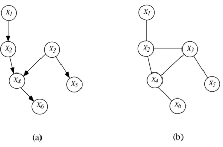
The structure of the model consists of specifying a set of conditional independence relations for the probabilistic model, or a set of (missing) edges in the graph for the graphical model. A UPIN structure species a set of conditional independence relations for a probability model in the form of an undirected graph. A DPIN structure species a set of conditional independence relations for a probability model in the form of a directed graph.
Inference and MAP Problems in HMMs
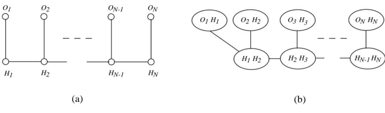
As mentioned earlier, this implies that the implicit independence properties of the DPIN structure are the same as those of the corresponding UPIN structure obtained by dropping the directions from the edges of the DPIN structure, and thus they both result in the same spanning tree structure (Figure 5b). . For the HMM(1,1) probabilistic model, the minimally directed and undirected graphs have the same Markov properties, i.e. imply the same conditional independence relations. The JLO algorithm applies to discrete valued variables: extensions to the JLO algorithm for Gaussian and Gaussian mixture distributions are discussed in Lauritzen and Wermuth (1989).
A closely related algorithm to the JLO algorithm, developed by Dawid (1992), solves the MAP identification problem with the same time complexity as the JLO inference algorithm. We show that the JLO and Dawid algorithms are strict generalizations of the well-known F-B and Viterbi algorithms for HMM(1,1), in that they can be applied to arbitrarily complex graph structures (and thus a large family of probabilistic models in addition to HMM) (1, 1)) and handle missing values, partial inference, and so on in a straightforward manner. However, it can be shown (Shachter et al. 1994) that all known exact algorithms for inference on DPINs are at some level equivalent to the JLO and Dawid algorithms.
Thus, it is sufficient to consider the JLO and Dawid algorithms in our discussion, as they are subordinate to other graphical inference algorithms. The second (propagation) step is performed each time a new inference is requested for the given graph.
The Construction Step of the JLO Algorithm: From DPIN structures to Junction Trees
Inference and MAP algorithms for DPINs and UPINS are quite similar: the UPIN case involves a number of subtleties not found in DPINs and therefore the discussion of UPIN inference and MAP algorithms is deferred to Chapter 7. inference algorithm for DPINs (developed by Jensen, Lauritzen, and Oleson (1990) and hereafter referred to as the JLO algorithm) is a descendant of an inference algorithm first described by Lauritzen and Spiegelhalter (1988). The construction step: This involves a series of sub-steps where the original directed graph is moralized and triangulated, a connecting tree is formed, and the connecting tree is initialized.
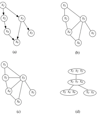
The propagation step: the junction tree is used in a local way by messages to propagate the consequences of observed evidence, i.e. to solve the inference and MAP problems. Thus, the JLO algorithm constructs a spanning tree by successively selecting a link of maximum weight unless it creates a cycle. The connection tree constructed from the cliques damped by the DPIN structure triangulation in Figure 7c is shown in Figure 7d.
The worst-case complexity is O(N3) for the triangulation heuristic and O(N2logN) for the maximum spanning tree part of the algorithm. This construction step is performed only once as an initial step to convert the original graph to a spanning tree representation.
Initializing the Potential Functions in the Junction Tree
Then, a tree of cliques will satisfy the continuous intersection property if and only if it is a spanning tree of maximum weight. From this point on, we will implicitly assume that the crossing tree has been initialized as described above, so that the potential functions are the local marginals.
Local Message Propagation in Junction Trees Using The JLO Algorithm
The collection phase involves forwarding ows along all edges towards the root clique (if a node is scheduled to have more than one incoming ow, the ows are absorbed sequentially). Once collection is complete, the distribution phase involves passing the efflux from this root in the reverse direction along the same edges. In a non-redundant arrangement, there are at most two ows along any edge in the tree.
Note that the directionality of the flows in the spanning tree is not necessarily related to any directed edges in the original DPIN structure.
The JLO Algorithm for Inference given Observed Evidence
Complexity of the Propagation Step of the JLO Algorithm
The F-B Algorithm for HMM(1,1) is a Special Case of the JLO Algo- rithm
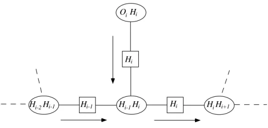
Let i;j =fOi;:::;Ojg denote a set of consecutive observable variables and i;j =foi;:::;ojg denote a set of observed values for these variables, 1i < j N. In particular, with using a "left-to-right" scheme the updated potential functions on the separators between the hidden cliques, the f1;i(hi) functions, are precisely the variables. Thus, when the JLO algorithm is applied to HMM(1 ,1), it produces exactly the same locally recursive computations as the forward phase of the FB algorithm.
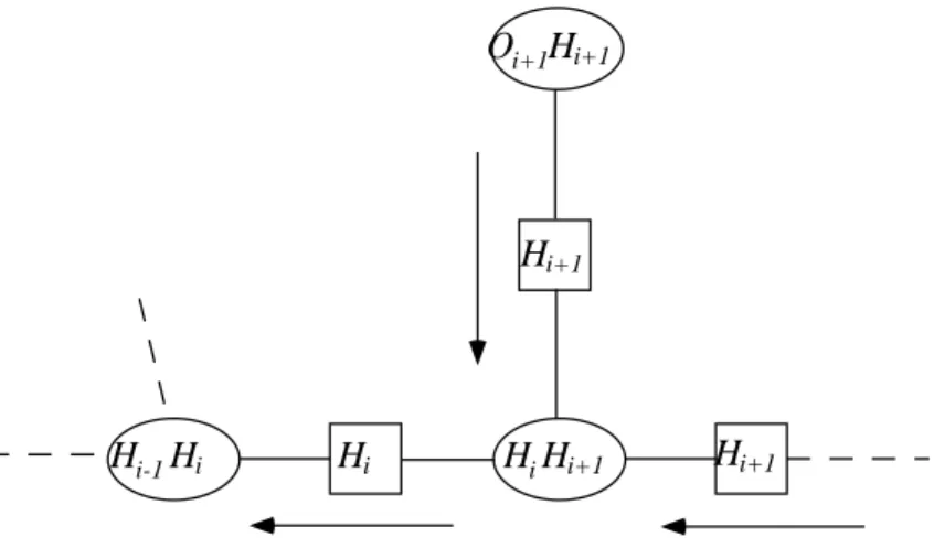
An equivalence can also be shown between the backward phase of the F-B algorithm and the JLO inference algorithm. Let the 'leftmost' clique in the chain (H1;H2) be the main clique and set up a schedule so that the flows flow from right to left. Recall that the cabal's potential (Hi;Hi+1) has already been updated by previous posts from the right.
Thus, we have shown that the JLO inference algorithm recreates the F-B algorithm for the special case of the HMM(1,1) probabilistic model.
Equivalence of Dawid's Propagation Algorithm for Identifying MAP As- signments and the Viterbi Algorithm
In the literature on probabilistic expert systems, this procedure is known as generating the "most likely explanation" (MPE) given the observed evidence. The HMM(1,1) MAP problem consists of providing a set of values for the observable variables, e= fO1 =o1;O2=o2;:::;ON =oNg and derive. Since Dawid's algorithm is applicable to any connection tree, it can be applied directly to the HMM(1,1) connection tree in Figure 5b.
The appendix shows that Dawid's algorithm, when applied to HMM(1,1), is exactly equivalent to the standard Viterbi algorithm.
Discussion of the Equivalences between the HMM and JLO Algorithms
For simplicity, we assume that all random variables are discrete (a Gaussian version of the IPF is also available (Whittaker 1990)), so that the joint distribution can be represented as a table. For each border in turn, the table is then scaled by multiplying each cell by the ratio of the desired border to the corresponding border in the current table. Jirousek and Preucil (1995) developed an efficient version of IPF that avoids the need to store the joint distribution as a table and avoids the need to explicitly marginalize the joint to obtain clique potentials.
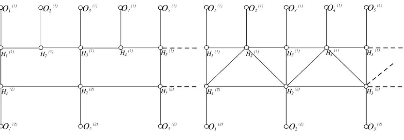
Various techniques have been developed to overcome these basic weaknesses of the HMM(1,1) model, including mixed emission probability modeling, triphone modeling, and discriminative training. The role of PINs is twofold: first, they provide a concise description of the probabilistic dependencies predicted by a particular model, and second, they provide a general algorithm for computing probabilities. Let Hi(1) and O(1)i denote the i-th state and i-th output of the \fast" chain respectively, and let Hi(2) and Oi(2) denote the i-th state and i-th output of the \slow" chain .
Formally, these induced dependencies are accounted for by links added between sequences of states during graph moralization (see Figure 11b). This figure shows that the basic calculations for this model are closely related to those of the previous HMM(1,2), but the model specification is very different in the two cases.
Parameter Estimation for PINs
More generally, the graphical modeling approach to the HMM(K,1) model allows the specification of different interaction matrices at different time scales; this is awkward in the Kth-order Markov chain formalism. Although discussion of averaging algorithms is beyond the scope of this paper, it is worth noting that the graphical modeling framework plays a useful role in the development of these approximations. In the E step, we calculate the expected sufficiency statistic for each of the parameters, given D and the current values for .
As mentioned, an important feature of the EM algorithm applied to PIN codes is that each term in the sum can be calculated using the JLO algorithm. The EM algorithm can also be used to find a local maximum of the posterior probability p(jD;M)/p(Dj;M)p(jM), where p(jM) is the prior parameter. Suppose the undirected model M consists of cliques Cij, so that the parameters of Ci1j and Ci2j are the same for i1 and i2.
In this case, we can estimate the parameters for the clique marginals, and then use Jirousek's IPF algorithm on a triangulation of M to compute a consistent estimate of the joint distribution. As in the directed case, we can use the JLO algorithm to perform the E-step:.
Model Selection and Averaging for PINs
Most often used priors are conjugate distributions, such as the Dirichlet distribution for the parameters of discrete variables and the mixing coefficients of Gaussian mixture codebooks, and the normal-Wishart distribution for the parameters of Gaussian codebooks (DeGroot 1970; Buntine 1994; Heckerman and Geiger 1995). Note that this score does not depend on the preceding parameter, and thus can be easily applied.1 For examples of applications of BIC in the context of PINs and other statistical models, see Raftery (1995). Other scores, which can be viewed as approximations of marginal likelihood, include hypothesis testing (Raftery 1995) and cross-validation (Fung and Crawford 1990).
In the context of HMM(K;J) type structures, an obvious question is how one could learn such a structure from data where K and J are unknown a priori. Using both the estimation techniques for a particular model described in the previous section (and the JLO algorithm for solving the E step as described in detail earlier in the paper) and the Bayesian (and alternative) model selection procedures outlined above, the algorithmic prescriptions for learning such models are in principle already in place. Probabilistic independence networks provide a useful framework for both analysis and application of multivariate probability models when there is significant structure in the model in the form of conditional independence.
The graphical modeling approach clarifies both model independence semantics and efficient computational algorithms for probabilistic inference. Trade relations between tongue body raising and lip rounding in the production of the vowel /u/: a pilot motor equivalence study.
The Viterbi Algorithm for HMM(1,1) is a Special Case of Dawid's Algorithm
Let Hi;j = fHi;:::;Hjg denote a set of consecutive observable variables and hi;j = fhi;:::;hjg denote the observed values for these variables, 1 i < j N.