Problems of optimal choice on posets and generalizations of acyclic colourings

(1)

Problems of optimal choice on posets and generalizations of

acyclic colourings

Bryn Garrod

Department of Pure Mathematics and Mathematical Statistics Trinity College

University of Cambridge

This dissertation is submitted for the degree of Doctor of Philosophy

3rd May 2011

(2)

(3)

For Rapha¨ele

(4)

(5)

Acknowledgements

I am very grateful to my supervisor, Béla Bollobás, for everything that he has done for me over the last three and a half years, from offering me professional assistance, support and advice to organizing research visits to the Rényi Institute in Budapest and to the University of Memphis. He has kept me going in the right direction when I have lost my way or my motivation, asked crucial questions when I have been stuck, and of course taught me and introduced me to a wealth of mathematical knowledge and understanding.

At the same time, he has become an integral part of my social life, whether sharing coffee and biscuits in the Pavilion E common room, or inviting me to parties or a Super Bowl in his home. I have enjoyed the many non-mathematical conversations that we have had, even if my lack of cultural knowledge is a constant disappointment!

I should like to thank my collaborators Grzegorz Kubicki, Micha l Morayne and Rob Morris. I am particularly grateful to Micha l and to Jan Tkocz for their warm hospitality when I visited them in Wroc law and to Rob for the help and advice that he has given me with my work far beyond his role as my departmental mentor. Thank you also to Graham Brightwell, whose discussions with B´ela and Rob led to an earlier proof of Theorem 3.2, for his helpful comments on the paper that I wrote with Rob, which became Chapter 3.

Thank you to Victor Falgas-Ravry for a useful conversation about Lemma 2.19. I hugely appreciate the constructive comments and corrections provided by my examiners, Andrew Thomason and Mark Walters.

I am grateful to the Engineering and Physical Sciences Research Council for funding me for the duration of my Ph.D. and to the Department of Pure Mathematics and Mathe- matical Statistics at the University of Cambridge for providing me with a very pleasant and productive working environment. Thank you to the organizers of the following confe- rences, all of whom supported my attendance financially, and also to the department, Trinity College and the London Mathematical Society for contributing to these costs:

v

(6)

vi ACKNOWLEDGEMENTS

the Bristol Summer School on Probabilistic Techniques in Computer Science, Building Bridges, the Fete of Combinatorics and Computer Science, the LMS-EPSRC Short Course on Probabilistic Combinatorics, the 22nd British Combinatorial Conference, the 14th In- ternational Conference on Random Structures and Algorithms, a conference in honour of the 70th birthday of Endre Szemer´edi, and the International Congress of Mathematicians 2010.

I have been very lucky with the people whom I have had to guide me through my mathematical studies. I am extremely grateful to my secondary school maths teacher, Peter Jack, for the encouragement and enthusiasm that he provided for more than seven years, and to Tim Gowers and Imre Leader for inspiring me in supervisions and lectures for the next seven.

Thank you to the rest of Team Bollob´as for the coffee times, mini-seminars and conference social life, particularly my good friends Tom Coker, Micha l Przykucki and Misha Tyomkyn. Thank you to all my other friends for their emotional support, particularly Jen Gold, Alex Holyoake, Phil Horler, C´eline Miani, Paul Smith, David Taylor, Charles Vial and Ioanna Vlahou, with whom I have spent most of my spare time over the last three and a half years.

I am hugely indebted to my parents, Martin and Dilys, and my sister and brother, Tania and Ross, for the happy, supportive family background in which I have grown up, and the encouragement that they have always given me.

My greatest thanks go to my wife, Rapha¨ele, whom I met at the start of my Ph.D.

and who is as much a part of it as the combinatorics. Thank you to her for marrying me and for looking after me so well. I am thankful for everything that she has done for me, which is more than I can write here.

(7)

Declaration of joint work

This dissertation is the result of my own work and includes nothing that is the outcome of work done in collaboration except where specifically indicated in the text. The first five sections of Chapter 2 are based on joint work with Grzegorz Kubicki¹ of the University of Louisville, USA, and Micha l Morayne²of Politechnika Wroc lawska, Poland, and about 50% of this is attributable to me. The work that forms the basis of Chapter 3 was joint with Robert Morris,³then of the University of Cambridge, UK, but now of IMPA, Brazil, and my contribution was about 75%.

1[email protected]

2[email protected]

3[email protected]

vii

(8)

(9)

Abstract

This dissertation is in two parts, each of three chapters. In Part 1, I shall prove some results concerning variants of the ‘secretary problem’. In Part 2, I shall bound several generalizations of the acyclic chromatic number of a graph as functions of its maximum degree.

I shall begin Chapter 1 by describing the classical secretary problem, in which the aim is to select the best candidate for the post of a secretary, and its solution. I shall then summarize some of its many generalizations that have been studied up to now, provide some basic theory, and briefly outline the results that I shall prove.

In Chapter 2, I shall suppose that the candidates come as m pairs of equally qualified identical twins. I shall describe an optimal strategy, a formula for its probability of success and the asymptotic behaviour of this strategy and its probability of success asm→ ∞. I shall also find an optimal strategy and its probability of success for the analagous version with c-tuplets.

I shall move away from known posets in Chapter 3, assuming instead that the candidates come from a poset about which the only information known is its size and number of maximal elements. I shall show that, given this information, there is an algorithm that is successful with probability at least ¹_e. For posets with k ≥2 maximal elements, I shall prove that if their width is alsok then this can be improved to ^k−1

q1

k, and show that no better bound of this type is possible.

In Chapter 4, I shall describe the history of acyclic colourings, in which a graph must be properly coloured with no two-coloured cycle, and state some results known about them and their variants. In particular, I shall highlight a result of Alon, McDiarmid and Reed, which bounds the acyclic chromatic number of a graph by a function of its maximum degree. My results in the next two chapters are of this form.

ix

(10)

x ABSTRACT

I shall consider two natural generalizations in Chapter 5. In the first, only cycles of length at leastlmust receive at least three colours. In the second, every cycle must receive at least ccolours, except those of length less than c, which must be multicoloured.

My results in Chapter 6 generalize the concept of a cycle; it is now subgraphs with minimum degree r that must receive at least three colours, rather than subgraphs with minimum degree two (which contain cycles). I shall also consider a natural version of this problem for hypergraphs.

(11)

Introduction

This dissertation is split into two unrelated parts. In Part 1, I shall consider several problems of optimal choice on posets, which are generalizations of a problem popularly known as the ‘secretary problem’. In Part 2, I shall consider generalizations of acyclic colourings of graphs, a concept whose origins can be traced back to Nash-Williams’s theorem concerning the decomposition of the edge set of a graph into forests.

Part 1: Problems of optimal choice on posets

The classical secretary problem is as follows. There arencandidates to be interviewed for a position as a secretary. They are interviewed one by one and, after each interview, the interviewer must decide whether or not to accept that candidate. If the candidate is accepted then the process stops, and if the candidate is rejected then the interviewer moves on to the next candidate. The interviewer may only accept the most recently interviewed candidate. At each stage, the interviewer knows the complete ranking of the candidates interviewed so far, all of whom are comparable, but has no other measure of their ability.

The interviewer is only interested in finding the very best candidate; selecting any other for the job is considered a failure. The aim is to find a strategy that maximizes the probability that the interviewer chooses the best candidate, under the assumption that the candidates are seen in a uniformly random ordering. In Chapter 1, I shall describe the solution to this problem, that there is a strategy that is successful with probability at least ¹_e and that this is asymptotically best possible. I shall also provide more of the historical background of this problem and some of its generalizations up to now.

In the rest of Part 1, I shall consider two generalizations of this problem. In Chapter 2, I shall first assume that there are 2mcandidates who are in factmpairs of identical twins, each pair of twins being equally well-qualified for the job. As in the classical problem, the interviewer knows at each stage how the candidates interviewed so far compare with each other, but has no other measure of their ability. I shall describe an optimal strategy, a

1

(14)

2 INTRODUCTION

formula for its probability of success and the asymptotic behaviour of this strategy and its probability of success asm→ ∞. I shall also find an optimal strategy and its probability of success for the analagous version on m sets of c-tuplets, and provide bounds that give some indication of their asymptotic behaviour.

I shall move from these known posets to unknown posets in Chapter 3. Specifically, I shall assume that the candidates come from a poset whose size nand number of maximal elements k is known, but whose structure is unknown. Here, the interviewer knows the poset induced by the candidates interviewed so far. I shall describe a strategy that is successful on all posets with given n and k with probability at least ¹_e, which is the best possible bound when k = 1, but probably not for k >1. I shall also find a strategy that is successful with probability at least ^k−1

q1

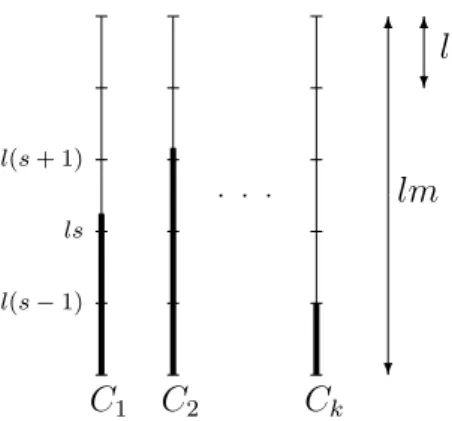
k when the width of the poset is known to be the same as the number of maximal elements k and k ≥ 2. By considering the poset consisting of k disjoint chains, I shall show that no greater probability of success can be guaranteed.

Part 2: Generalizations of acyclic colourings

An acyclic colouring of a graph is a proper vertex-colouring such that every cycle contains vertices of at least three colours. To put it another way, it is an assignment of colours to the vertices such that the graph induced by the vertices in any colour class must be an independent set, and the graph induced by the vertices in any two colour classes must be a forest. The acyclic chromatic number of a graph is the minimum number of colours needed to colour it acyclically. In Chapter 4, I shall describe how this concept came into being as a generalization of the arboricity of a graph, which is the minimum number of forests into which its edge set can be decomposed, and I shall state some of the many results proved about acyclic colourings up to this point. In particular, I shall highlight a result of Alon, McDiarmid and Reed, which bounds the acyclic chromatic number of a graph by a function of its maximum degree. My results in Part 2 will be of this form.

In Chapter 5, I shall consider two generalizations in which the subgraphs under scru- tiny are still cycles. In the first, the extra condition that a proper colouring must satisfy is relaxed so that only cycles of length at least l must receive three colours, that is, the

(15)

PART 2: GENERALIZATIONS OF ACYCLIC COLOURINGS 3

graph induced by the vertices in any two colour classes does not contain a cycle of length at leastl. In the second, I shall strengthen the condition so that every cycle must receive at least ccolours, with the obvious exception of cycles of length less than c, which must be multicoloured. In this case, the graph induced by the vertices in any x colour classes with x < c does not contain any cycles of length greater thanx.

The definitions given so far would work just as well if ‘cycle’ were replaced by ‘2-regular subgraph’ or even ‘subgraph with minimum degree at least 2,’ since cycles fall into both of these categories and any subgraph of either type must contain a cycle. I shall focus my attention in Chapter 6 on subgraphs with minimum degree r; a graph contains at least as many of these as r-regular subgraphs, and indeed is unlikely to have any r-regular subgraphs for larger, so this is more restrictive. In a proper colouring, it is possible for any bipartite subgraph with minimum degreer to receive only two colours; I shall insist that it receive three. I shall also consider the same problem for u-uniform hypergraphs, under the assumption that a proper colouring is one in which every edge is multicoloured.

(16)

(17)

Part 1 Problems of optimal choice on posets

(18)

(19)

CHAPTER 1

The classical secretary problem

1.1. The problem

The exact origins of the classical secretary problem are complicated (and the subject of Ferguson’s history of the problem [26]), but the problem was popularized by Martin Gardner [32, 33] in his Scientific American column in February 1960, as the game goo- gol. The problem itself is simple to state, and its ‘secretary problem’ formulation is as follows. There aren candidates to be interviewed for a position as a secretary. They are interviewed one by one and, after each interview, the interviewer must decide whether or not to accept that candidate. If the candidate is accepted then the process stops, and if the candidate is rejected then the interviewer moves on to the next candidate. The interviewer may only accept the most recently interviewed candidate. At each stage, the interviewer knows the complete ranking of the candidates interviewed so far, all of whom are comparable, but has no other measure of their ability. The interviewer is only interested in finding the very best candidate; selecting any other for the job is considered a failure. The aim is to find a strategy that maximizes the probability that the interviewer chooses the best candidate, under the assumption that the candidates are seen in a uniformly random ordering.

1.2. Outline solution

The solution to the classical secretary problem is now folklore but was first published by Lindley [57], and I shall give an outline of it here.

It is obvious that the interviewer should only consider accepting a candidate who is the best seen so far. It is intuitively clear that a candidate should not be accepted very early on even if he or she is the best seen so far, since there is a reasonable probability that a small number of candidates all come from near the bottom of the ranking. Conversely, the interviewer should not wait too long, or the best candidate will probably be missed and

7

(20)

8 1. THE CLASSICAL SECRETARY PROBLEM

the interviewer will not have the opportunity to select anyone. Furthermore, if a strategy dictates that the i^th candidate should be accepted if he or she is the best candidate seen so far, it seems reasonable that the (i+1)^th should be accepted in the same circumstances, since more candidates have been seen and that candidate’s credentials are stronger. From these observations, it might be expected that some sort of threshold should be passed before the interviewer considers choosing a candidate.

Using backward induction, one can prove exactly that. This will be described in more detail in Section 1.5; for now, I shall assume the following consequence of it without proof.

For some k, the strategy “reject the first k candidates, and accept the next who is the best seen so far” is optimal. As an aside, it is worth noting that there might be more than one optimal strategy: for example, when there are exactly two candidates, the two possible deterministic strategies are equivalent, and both are equivalent to tossing a coin to choose between the two candidates.

LetW be the event that, using this strategy, the interviewer chooses the best candidate and letBi be the event that thei^thcandidate interviewed is the best candidate. LetAi be the event that the interviewer is still interviewing by the time the i^th candidate arrives, that is, that the best of the firsti−1 candidates interviewed is in the first k interviewed.

Then B_i and A_i are independent, and the probability of winning is given by P(W) =

n

X

i=k+1

P(B_i)P(W|B_i)

=

n

X

i=k+1

P(B_i)P(A_i)

=

n

X

i=k+1

1 n · k

i−1

= k n

n−1

X

j=k

1 j. A value ofk that maximizes this satisfies

k n

n−1

X

j=k

1

j ≥ k−1 n

n−1

X

j=k−1

1

j and k

n

n−1

X

j=k

1

j ≥ k+ 1 n

n−1

X

j=k+1

1 j,

(21)

1.3. VARIANTS 9

that is,

n−1

X

j=k

1

j ≥ k−1

k−1 = 1 and

n−1

X

j=k+1

1 j ≤ k

k = 1, from which simple integration arguments give

n

e −1≤k≤ n

e + e−1 e . From this, it is clear that for suchk

n→∞lim k n = 1

e

and that the probability of winning tends to the same limit. In fact, in Chapter 3, it will become evident that this is a lower bound.

1.3. Variants

A problem posed by Cayley [18] may have inspired the classical secretary problem.

This is what is now known as the ‘full information’ case, where the candidates’ abilities are represented by real random variables from a known distribution, and the aim is to maximize the expected ability of the chosen candidate. The uniform distribution U[0,1]

was considered by Moser [62]; Guttman [46] found an optimal strategy for a general distribution and also gave an explicit optimal strategy for the normal distributionN(0,1).

His general optimal strategy is to accept a candidate if there are at least m candidates remaining after that one and his or her ability is at least E_m, for some (E_m)m∈N. For U(0,1), the first few values ofE_m are 0.5, 0.625, 0.6953, 0.7417 and 0.775, and forN(0,1) they are 0, 0.3992, 0.6298, 0.7904 and 0.9127. The expected ability is the first threshold for acceptance,E₁.

Since 1960, many generalizations of the classical secretary problem have been considered. Freeman [28] wrote an extensive review of the area in 1983, which shows how many versions had already been considered by then. I shall describe only some of them, and some more recent results.

Besides the full information case, the most obvious generalization might be to be more flexible over what constitutes success, and to try to minimize the expected rank (viewing the best candidate as being from rank 1 and the worst from rankn) rather than insisting

(22)

on choosing the best candidate. This version was solved by Chow, Moriguti, Robbins and Samuels [21]. Perhaps surprisingly, in the limit as n → ∞ the optimal expected rank tends to a constant rather than a multiple of n, namely,

∞

Y

j=1

j + 2 j

_j+1¹

≈3.8695.

They showed that an optimal strategy is to accept a candidate who is in the top kseen so far as long as at least ik candidates have been seen in total, for some thresholds ik. They also showed that the i_k satisfy

n→∞lim i_k n =

∞

Y

j=k

j j+ 2

_j+1¹ .

This means that, for large n, once we have seen approximately 26% of candidates we should be prepared to accept the next one who is the best so far, after 45% we should accept anyone who is one of the top two seen so far, after 56% one of the top three, after 64% one of the top four, after 69% one of the top five and so on. At the other end of the scale, once we have seen 99% of candidates we should accept anyone who is in the top 200 and after 99.9% anyone in the top 2000.

Yang [80] considered the situation where, as well as being allowed to offer the job to the most recently interviewed candidate, who would accept it, the interviewer can offer the job to any of the other candidates seen so far, who is still available with probability q(r), whereqis a known non-increasing function of the numberrof candidates interviewed since that one. If a candidate is unavailable, he or she never becomes available again. The aim is to choose the best possible secretary, as in the classical secretary problem. Smith [74]

studied a version where the job can only be offered to the currently interviewed candidate, but there is some fixed probability that the candidate will refuse the offer. Petruccelli [67]

worked on these two problems simultaneously, that is, Yang’s problem withq(r) still non- increasing but with q(0) no longer forced to be 1.

In particular, Petruccelli considered the case where the probabilities form a geometric progression, that is, where q(r) = qp^r for some p and q. He proved that there are two cases, depending on p, q and the number n of candidates. If P∞

r=0q(r) = _1−p^q > n−1 then an optimal strategy is to observe all n candidates and then to offer the job to the

(23)

1.3. VARIANTS 11

best one. If _1−p^q ≤ n−1, then an optimal strategy is to wait until s_n candidates have been seen, for some s_n, and then to offer the job to the best one seen so far. If this one is unavailable, then the interviewer should continue interviewing and offer the job to the next candidate who is the best seen so far. If this one is unavailable, then the interviewer should continue as before, and so on. He gave an explicit formula for s_n, namely, the smallest value ofs for which

n−1

Y

k=s+1

1 + 1−q k

≤

q

1 + 1−q s(1−p)

−1

.

He also showed that both ^s_nⁿ and the probability of success tend to q^1−q¹ as n→ ∞. This is independent of p, which means that for largen there is effectively no benefit to being allowed to recall a previous candidate, since p can be arbitrarily small. However, this is not surprising, since if p is fixed then only a constant number of candidates are likely to be available at any one point, even as n→ ∞.

Gusein-Zade [45] allowed selection of any of the top r candidates to count as success, and showed that an optimal strategy is of the same form as in the expected rank case, that is, an optimal strategy is to accept a candidate who is in the top k seen so far as long as at leasti_k candidates have been seen in total, for some thresholds i_k. He showed that forr = 2 the limiting probability of success as n → ∞ is about 0.5736. Frank and Samuels [27] proved that the optimal probability of success p(n, r) satisfies

r→∞lim lim

n→∞ 1−p(n, k)¹_r

= 1−t^∗, where t^∗ = lim

n→∞

i₁

n ≈0.2834.

Gilbert and Mosteller [40] considered what could be called the inverse of this problem:

the interviewer is allowed to pick up to r candidates and wins if any of them is the best.

(Many other variations of the secretary problem are included in the same paper.) They showed that an optimal strategy is to wait until t(n, r) candidates have been seen, for some functiont(n, r), then to pick the next who is the best seen so far, and then to play an optimal strategy for the remaining candidates andr−1 choices. They found an iterative method to calculate the limits

u_r = lim

n→∞

t(n, r) n ,

(24)

showed that the first few values of u_r are e⁻¹, e⁻³², e⁻⁴⁷²⁴ and e⁻²⁷⁶¹¹¹⁵², and showed that as n → ∞the optimal probability of success tends to

r

X

i=1

u_i.

Some authors wondered what would happen if the number of candidates were unknown, but the distribution of that number, the random variableN, were known. Presman and Sonin [69] found an explicit optimal strategy for a general distribution, where the aim is to choose the best candidate. They also showed that if the number of candidates is uniform in [n], then an optimal strategy is of the same form as in the classical secretary problem, but where the threshold is asymptotically equivalent to _eⁿ2 and the probability of success tends to _e²2 ≈0.2707 as n→ ∞.

Gianini-Pettitt [39] considered the minimal expected rank version of this problem, and restricted her attention to distributions of the form

P N =x

N ≥x

= (n−x+ 1)^−α,

for some α. She proved that, as when the number of candidates is known, an optimal strategy is of the form ‘accept the i^th candidate if it is one of the best k(i) seen so far,’

but that k(i) is not necessarily an increasing function. She also proved the surprising fact that if N₁ and N₂ are possible distributions of the number of candidates and N₁ is stochastically smaller than N₂, that is, P(N₁ ≤ x) ≥ P(N₂ ≤ x) for all x, this does not imply that the minimum expected rank decreases. One example of this is that if N₁ is uniformly distributed on [n], that is, if α = 1, then the optimal expected rank tends to infinity as n → ∞, whereas if N₂ = n with probability 1 then, as shown by Chow, Moriguti, Robbins and Samuels [21], the optimal expected rank tends to about 3.8695.

In fact, she showed that the optimal expected rank tends to infinity if α < 2 and to the Chow, Moriguti, Robbins and Samuels limit of approximately 3.8695 if α > 2, and if α = 2 then the lim inf of the optimal expected rank is greater than 3.8695 and the lim sup is finite.

More generally, one could consider problems of optimal choice on more complicated systems; up to this point the assumption has always been that there are n rankable

(25)

1.3. VARIANTS 13

candidates. Kuchta and Morayne [56] considered a version of the classical secretary problem where the interviewer has k ‘lives’: if all n candidates are interviewed without any of them being chosen, then a new set of n candidates is interviewed, and the aim is to chose the best of these, and so on. At most k sets of candidates are allowed to be interviewed in total. They showed that, for some function t(n, k), an optimal strategy is to ignore the first t(n, k) candidates from the first set, and accept the next candidate who is the best seen so far; if no such candidate appears, then ignore the firstt(n, k−1) candidates from the next set and accept the next candidate who is the best seen so far, and so on. They showed that

n→∞lim

t(n, k) n

exists, and denoting it bya_k, that a_k+1 =e^a^k⁻¹, where of course a₁ = ¹_e.

Stadje [75] introduced the idea that the candidates could be ranked separately in each ofk >1 different criteria, with the interviewer wishing to select a candidate who is maximal in at least one of them, and Gnedin [41] solved the version where these rankings are random and independent of each other. He proved that an optimal stratgy is to wait until a certain number of candidates have been seen and then to select the next who is best according to at least one criterion, and that the limiting values of this threshold and the probability of success are both ^k−1q

1

k. Gnedin has also produced a more general survey of multicriteria problems [42]. In fact, these last two problems could both be viewed as versions of the secretary problem on k disjoint chains, which I shall solve in Chapter 3, with an extra restriction, about which I shall say more at the time.

Moving slightly further away from the classical secretary problem, Kubicki and Mo- rayne [55] considered the problem on a directed path, where at each stage the selector knows the directed graph induced by the vertices seen so far and wishes to choose the end-vertex with no edge going out of it. This is similar to the classical secretary problem, but each candidate can only be compared with the one immediately above it or below it in the ranking. They showed that an optimal strategy is to wait until the first timetwhen the induced graph hasn−t+ 1 connected components and to pick the t^th vertex. Note that this is the first time when the selector can be sure that the sought after end-vertex has been seen: if at timet the induced graph has n−t+ 1 connected components, then

(26)

the remaining n−t vertices must be used to join components together, and so none of them is the end-vertex. Note also that this strategy is independent of whether or not the t^th vertex is an end-vertex of its component; if it is not, then it does not make any difference which vertex is chosen. They showed that the probability of successp_n satisfies

n→∞lim p_n√ n =

√π 2 .

Przykucki and Sulkowska [71] adapted this problem in a similar way to Gusein-Zade’s version of the classical secretary problem, so that choosing the end-vertex or its neighbour counts as success. In this case, the optimal stopping time and its analysis are more complicated, but their numerical analysis shows that the probability of success behaves approximately like ^1.26^√_n. For comparison with the previous result,

√π

2 ≈0.8862.

s

s s s

s s s s s s s s s

s s s s s s s s s s s s s s s s s s s s s s s s s s s 1

6

PP PP P i

PP PP P

6 6 6

@

@ I

@

@ I

@

@ I

@@

6 6 6 6 6 6 6 6 6

BB M BMB

BB M

B

B B B

B B

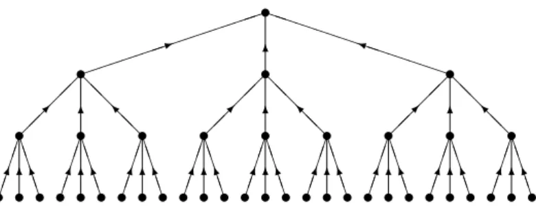
Figure 1.1. Directed ternary tree of depth 3.

Morayne and Sulkowska [61] studied a variation of the directed path version, in this case working with the completek-ary directed rooted tree of depthn (see Figure 1.1) and again assuming that the selector knows the induced directed graph at each stage of the process. They found a lower bound for the probability of success of an optimal strategy by considering a natural (but not necessarily optimal) strategy: select the currently examined element if there is a directed path of lengthn terminating at it. If this ever happens, then the strategy must be successful. In this way, they showed that on a binary tree the limit of the optimal probability of success is at least 2 log 2−1≈0.3863 and that on a ternary tree it is at least ³₂log 3−2 + ₂^√^π₃ ≈0.5548, and that it tends to 1 as k → ∞.

Przykucki [70] posed a problem concerning the random graph G_n,p with n vertices and any two connected by an edge with probabilitypindependently of the others. Again, the selector knows the graphs induced by the vertices seen so far, and wishes to find a vertex of full degree, that is, degree n−1. He showed that an optimal strategy is to wait

(27)

1.3. VARIANTS 15

untilk(n, p) vertices have been seen and then to pick the next vertex connected to every vertex seen so far, for somek(n, p). He showed that, for fixed p∈(0,1),

k(n, p) = log¹

pn+O(1)

asn → ∞, and found a formula for the probability of its success, which of course tends to zero more quickly thannpⁿ⁻¹, which is an upper bound for the probability that a vertex of full degree exists.

In this dissertation, the type of generalization that I shall consider is to put partial orders other than a total order on the candidates. Here, the selector knows the poset from which the elements are taken and the poset induced by the elements observed so far, and wishes to choose an element that is maximal in the ground poset.

s

s s

s s s s

s s s s s s s s

s s s s s s s s s s s s s s s s

H HH

HH HH

H

@

A

A A

A

A A

C

C C

C

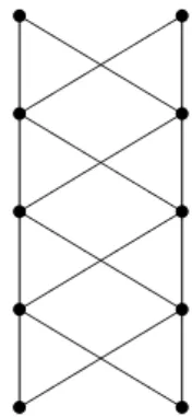
Figure 1.2. Binary tree of depth 4.

A generalization due to Morayne [60] is to consider the case of a binary tree of depth n (see Figure 1.2). Intuitively, it seems unlikely that a random selection of nodes would come from a subtree with a maximum other than the global maximum unless they are linearly ordered, and he showed that this is indeed the case. An optimal strategy here is to select the maximum out of the elements seen so far when the poset induced by these elements is either linear of length greater than ⁿ₂ or non-linear with a unique maximum.

He showed further that as n→ ∞, the probability of success tends to 1.

Ka´zmierczak [49] added a ‘witness’ to the classical secretary problem, an extra element win the poset that lies immediately below the maximal element but cannot be compared with any other element. Tkocz [77] extended this concept to put the witness below the

(28)

s

s s s s s

b b

b

x1

x_k

x_n

w

Figure 1.3. Tkocz’s poset.

k^th highest element (see Figure 1.3). He gave an explicit optimal strategy, which uses three different thresholds, essentially depending on the size ofk relative ton. If the poset induced by the elements seen so far is linear and of length greater than the threshold then a maximal element should be accepted; if it is not linear then an optimal strategy for the classical secretary problem on k elements should be followed. He also calculated the asymptotic probabilities of success for k = 2 and 3, approximately 0.415 and 0.384 respectively, compared with the figure of approximately 0.573 for k = 1 obtained by Ka´zmierczak.

s s s s s

"

""

"

b b

b b b

b b

b b b

b b

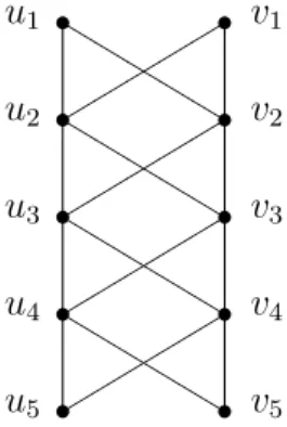
Figure 1.4. Five pairs of identical twins.

Micha l Morayne, Grzegorz Kubicki and I [34] considered the case ofmpairs of ‘twins’, where there are mlevels with two incomparable elements on each level (see Figure 1.4); I shall present these results in Chapter 2. I shall show that an optimal strategy is to wait until elements from a certain threshold number of levels have been seen and then to select the next element that is maximal and whose twin has already been seen. I shall further show that as m → ∞, this threshold behaves roughly like 0.4709m and the probability of success tends to approximately 0.7680. Calculating these asymptotic values for the

(29)

1.3. VARIANTS 17

natural extension to ‘c-tuplets’ for c > 2, is a harder problem, and I shall provide some bounds.

A further interesting generalization, due to Preater [68], was an attempt to find an algorithm that was successful onall posets of a given size with positive probability. Sur- prisingly, he proved that there is such a ‘universal’ algorithm (depending only on the size of the poset), which is successful on every poset with probability at least ¹₈. In this algorithm, an initial random number of elements are rejected and a subsequent element is accepted according to randomized criteria. A slightly modified version of the algorithm, also suggested by Preater, was analysed by Georgiou, Kuchta, Morayne and Niemiec [36], and gave an improved lower bound of ¹₄ for the probability of success. More recently, Kozik [54] introduced a ‘dynamic threshold strategy’ and showed that it was successful with probability at least ¹₄ +ε, for someε >0 and for all sufficiently large posets. When I was about to submit this dissertation, Micha l Morayne drew my attention to a very recent paper of Freij and W¨astlund [29]. In it, they describe a strategy that is successful with probability at least ¹_e. This cannot be improved, since the best possible probability of success in the classical secretary problem, on a totally ordered set, is ¹_e. I shall say more about this in Section 3.4.

Before Kozik, Freij and W¨astlund had published their results, Robert Morris and I [35]

showed that, given any poset, there is an algorithm that is successful with probability at least ¹_e, so, in this sense, the total order is the hardest possible partial order. I shall present these results in Chapter 3. In fact, this algorithm depends only on the size of the poset and its number of maximal elements, so it is universal for any family where these are given. It is therefore natural to ask which is the hardest partial order with a given number of maximal elements. The most obvious choice is the poset consisting of k disjoint chains. I shall give an asymptotically sharp lower bound on the probability of success in the problem of optimal choice onk disjoint chains, and show that it is at least as hard as on any poset with k maximal elements and of width k, that is, whose largest antichain has sizek.

(30)

1.4. Formal model and notation

In this section, I shall define formally the probability space in which I shall work in Chapters 2 and 3.

This probability space will depend on a poset (P,≺) with P = {x₁, . . . , x_n}. In Chapter 2, this will be a known poset, the poset of m pairs of identical twins or, later, m sets of identical c-tuplets. In Chapter 3, this will be a fixed but unknown poset. Let max≺(P) denote the set of its maximal elements, that is,

max≺(P) = {x∈P :6 ∃y such that x≺y}.

The subscript in max_≺ will be suppressed when it is clear from the context.

Given (P,≺), I shall work with a probability space (Ω_P,F_P,PP), with EP defined in the obvious way. The subscripts will be suppressed when they are clear from the context, as they will be for the rest of this section. The probability space (Ω,F,P) is defined as follows. Set Ω =S_n×[0,1], whereS_nis the permutation group on [n], andF =P(S_n)×B, whereBis the Borelσ-algebra. LetP=µ×λ, whereµis the uniform probability measure, that is,

µ({ρ}) = 1 n!

for all ρ ∈ S_n, and λ is the Lebesgue measure. In other words, (ρ, δ) ∈ Ω is picked uniformly at random. Given (ρ, δ)∈Ω, theρ-co-ordinate will determine the order in which elements of P appear and the δ-co-ordinate will allow the introduction of randomness independent of this order into our algorithms. This will not be needed in Chapter 2; in Chapter 3, theδ-co-ordinate will determine an initial number of elements to reject without considering. The reason why continuous space and Lebesgue measure are used, despite the fact that all of the randomized strategies considered pick one of a finite number of options, is that this allows them all to lie in the same probability space.

Write P^[n] for the set of permutations of P, and let π : Ω → P^[n] be the random variable defined by

π(ρ, δ)(i) =x_ρ(i).

(31)

1.4. FORMAL MODEL AND NOTATION 19

LetPtdenote the set of all posets with vertex set [t] ={1, . . . , t}. Let (P_t)t∈[n]be a family of random variables withP_trepresenting the poset seen at time t. Formally,P_t: Ω→Pt

and eachP_t(ρ, δ) = ([t],≺_t) is defined by

∀i, j ∈[t], i≺_tj ⇐⇒π(i)≺π(j).

The poset P_t is the natural description of what is seen at time t as the elements of P appear one by one.

Let (F_t)t∈[n] be the sequence of σ-algebras with each F_t generated by the random variablesP₁, . . . , P_t, that is,

F_t=σ(P₁, . . . , P_t) = σ(P_t),

the second equality holding sincePt is a labelled poset and thus its value determines the values of P₁, . . . , Pt−1. The σ-algebra F_t can be thought of as the information known at time t about where we are in the universe Ω. Since P_t takes only finitely-many values, Ft has a simple structure; it is the pre-images in Ω of the possible values of Pt and the unions of these pre-images. These pre-images are called the atoms of F_t.

LetF_t⁰ be the projection ofF_tontoP(S_n). Since definitions have so far depended only on theρ-co-ordinate of (ρ, δ)∈Ω, it is clear that, for each t,

F_t={A×[0,1] :A∈ F_t⁰}.

In other words, (ρ₁, δ₁) and (ρ₂, δ₂) are in the same atom of F_t if and only if ρ₁ and ρ₂ are in the same atom ofF_t⁰, which happens if and only if the labelled posets induced by the firstt elements π(1), . . . , π(t) are identical.

Astopping time is a random variableτ taking values in [n] and satisfying the property {τ =t} ∈ F_t,

that is, the decision to stop at time t is based only on the values of P₁, . . . , P_t.

I shall give a brief reminder of the formal definitions of conditional expectation and probability, which in the finite world are intuitive concepts. For more details, see page 304 of Galambos [30] or page 313 of Chung [23], for example. Let X be a random variable.

(32)

Then theconditional expectation ofX givenF_t, denoted byE(X|F_t) is anyF_t-measurable random variable satisfying

Z

A

E X F_t

= Z

A

X for all A∈ F_t.

Any two random variables satisfying these conditions are equal with probability 1. AsF_t is finite, this random variable is constant on each atom of F_t and takes the average value of X on that atom, that is,

E X F_t

(ω) = R

AX

P(A) =E(X|A),

where A is the atom of F_t containing ω. In the same way that the probability of an event E is the expectation of the indicator function 1(E) of this event, the conditional probability of E givenFt is defined by

P E F_t

=E 1(E) F_t

, that is, since F_t is finite,

P E F_t

(ω) = E 1(E) F_t

(ω) = R

A1(E)

P(A) = P(A∩E)

P(A) =P(E|A), where A is the atom of F_t containingω.

Define the family of random variables (Z_t)t∈[n] by Z_t =P π(t)∈max(P)

F_t ,

that is, the random variable Z_t is the probability that the t^th element observed is maximal given P₁, . . . , P_t. The general aim will be to choose stopping times τ to maximize P π(τ) ∈max(P)

. This quantity is equal to E(Zτ) (see page 45 of Chow, Robbins and Siegmund [22], for example):

E(Zτ) = Z

Ω

Zτ =

n

X

t=1

Z

{τ=t}

Zt=

n

X

t=1

Z

{τ=t}P π(t)∈max(P) Ft

=

n

X

t=1

Z

{τ=t}

1 π(t)∈max(P)

= Z

Ω

1 π(τ)∈max(P)

=P π(τ)∈max(P) ,

(33)

1.5. USEFUL THEOREMS 21

the fourth equality holding by the definition of conditional expectation since{τ =t} ∈ F_t. These equivalent formulations will be useful later; this conditional probability can be treated as a pay-off offered at each step of the process.

Recall that F_t⁰ is the projection of F_t onto P(S_n). A randomized stopping time is a random variable τ taking values in [n] and satisfying the property

{τ =t} ∈ F_t⁰× B,

that is, the decision to stop at timet is based on the values of P₁, . . . , P_t and on some B- measurable random variable. The randomized stopping times considered in Chapter 3 will be convex combinations of a finite number of true stopping times, so if such a randomized stopping time gives a certain probability of success, then there is a true stopping time with at least that probability of success. In fact, this is true in general, as proved by Ghoussoub [38].

1.5. Useful theorems

In this section, I shall define backward induction formally and use it to solve the classical secretary problem. I shall also state a theorem that gives an optimal stopping time for monotone processes, to be defined later.

The next theorem, which is proved as Theorem 3.2 on page 50 of Chow, Robbins and Siegmund [22], gives in principle an optimal stopping time for any finite process, although in practice it might be hard to define such a stopping time more explicitly. It formalizes the concept of backward induction. Informally, it can be described is as follows.

Define a new random variable for each t, thevalue of the process at timet. This is the expected pay-off ultimately accepted given what has happened so far. These values are calculated inductively, starting at the end. The value of the process at the final step is just the final pay-off offered. The value of the process at each earlier step is the maximum of the currently offered pay-off and the expected value of the process at the next step.

An optimal strategy is to stop when the currently offered pay-off is at least the expected value at the next step.

In the theorem below, the pay-offs offered are the W_t and the values at each step are the γ_t. The σ-algebras A_t represent what is known at time t. As a reminder, being

(34)

A_t-measurable means that σ(W_t)⊂ A_t, that is, the value of W_t is determined by what is known at time t or, in the finite world, W_t is constant on each atom of A_t. In fact, the nested condition means that A_t ⊃σ(W₁, . . . , W_t). The conclusion of the theorem is that the strategy that stops at the first t when W_t =γ_t (or, equivalently, whenW_t is at least as large as the expected value of γ_t+1 given A_t) is indeed a stopping time and achieves the optimal value.

Theorem1.1.LetA₁ ⊂. . .⊂ A_nbe a nested sequence ofσ-algebras and letW₁, . . . , W_n be a sequence of random variables with eachW_t beingA_t-measurable. LetC_(A_t₎ be the class of stopping times relative to (A_t)t∈[n] and let v^∗ be given by

v^∗ = sup

τ∈C_(A

t)

E(Wτ).

Define successively γ_n, γn−1, . . . , γ₁ by setting γ_n=W_n,

γ_t= maxn

W_t,E γ_t+1 A_to

, t=n−1, . . . ,1.

Let

τ^∗ = min{t:W_t=γ_t}.

Then τ^∗ ∈ C(A_t) and

E(W_τ^∗) = E(γ₁) =v^∗ ≥E(W_τ) for all τ ∈ C(At).

This theorem can now be used to justify the assertion in Section 1.2 that an optimal strategy is of the form “reject the firstk candidates, and accept the next who is the best seen so far.” Recall from Section 1.4 that

Z_t =P π(t)∈max(P) F_t

,

that is, the probability that thet^th candidate is the best one given what is known at this point. Backward induction will be applied with the Z_t corresponding to theW_t, with F_t toG_t and with δ_t to γ_t.

(35)

Since the random variables Z_t are independent, the values of Z₁, . . . , Z_t give no information about the values ofZ_t+1, . . . , Z_n, and thereforeE(δ_t+1|F_t) is constant on all atoms of F_t and equal to E(δ_t+1). Therefore, define the functionv : [n]→R by

v(t) = E(δ_t)

and note that backward induction tells us that the stopping time that stops at the first t such thatZ_t ≥E(δ_t+1|F_t) =v(t+ 1) is optimal. By definition,

v(t) = E max{Z_t, v(t+ 1)}

≥v(t+ 1),

whereas _n^t, the potential non-zero value ofZ_t, is a non-decreasing function oft. Therefore, there exists k such that

t

n < v(t+ 1) if t≤k, t

n ≥v(t+ 1) if t > k,

and an optimal strategy is “reject the firstk candidates, and accept the next who is the best seen so far,” as claimed.

In fact, this argument is not even necessary, as the classical secretary problem is a sufficiently straightfoward process that backward induction can be used to give an explicit optimal strategy. This is because in this case theδt can be calculated explicitly, as in the next lemma, and these define an optimal strategy.

Lemma 1.2. For all t≤n, if

n

X

i=t

1 i ≤1, then

E δ_t F_t−1

= t−1 n

n−1

X

i=t−1

1 i,

that is, it is the constant random variable taking that value; otherwise,

E δ_t Ft−1

=E δ_t+1 F_t

.

(36)

Proof. By definition, δ_n =Z_n and so E δ_n

F_n−1

= 1

n = n−1

n · 1

n−1. Fort ≤n−1, if

t n ≥ t

n

X

i=t

1

i =E δ_t+1 F_t

, then

E δ_t Ft−1

=P

Z_t ≥E δ_t+1 F_t

·E

Z_t

Z_t ≥E(δ_t+1|F_t) +P

Z_t<E δ_t+1 F_t

·E

E(δ_t+1|F_t)

Z_t<E(δ_t+1|F_t)

(1.1)

= 1 t · t

n + t−1 t · t

n

n−1

X

i=t

1 i

= t−1 n

n−1

X

i=t−1

1 i. If

t n < t

n

X

i=t

1

i =E δt+1

Ft

, then, from the formula in (1.1), it is the case that

E δ_t Ft−1

= 0· t

n + 1·E δ_t+1 F_t

=E δ_t+1 F_t

.

This lemma and the backward induction theorem clearly give the same optimal stopping time as before: accept thet^thcandidate if he or she is the best so far and Pn

i=t 1 i >1.

The other main tool used in Part 1 of this dissertation is the most basic result for infinite processes. It is used in Chapter 2 for the reason that the twins case will be reduced to a process that, although finite, does not have a fixed number of steps, and so backward induction is inappropriate. The following theorem is slightly adapted from that on page 55 of Chow, Robbins and Siegmund [22], since the random variables of interest are all positive.

(37)

This theorem applies only to the monotone case, and monotonicity is a strong property: it is the property that, after the first time in the process where the currently offered pay-off is at least the expected pay-off at the next step, the same is true at all future times. The conclusion of the theorem is that the first time when this is true is an optimal stopping time.

Theorem1.3. LetA₁ ⊂ A₂ ⊂. . .be a nested sequence ofσ-algebras and letW₁, W₂, . . . be a sequence of random variables with eachW_tbeingA_t-measurable. LetC(At) be the class of stopping times relative to(A_t)_t∈[n]. For t∈N, let

A_t=n

E W_t+1 A_t

≤W_to . and suppose that

A₁ ⊂A₂ ⊂. . . and

∞

[

t=1

A_t = Ω. (1.2)

Let

τ^∗ = minn

t:W_t≥E W_t+1 A_to

. Suppose that P(τ^∗ <∞) = 1 and E(W_τ^∗) exists and that

lim inf

t

Z

{τ^∗>t}

Wt= 0.

Then

E(W_τ^∗)≥E(W_τ) for all τ ∈ C(At).

If equation (1.2) holds then the process (Wt,At)t∈[n] is said to be monotone.

(38)

(39)

CHAPTER 2

How to choose the best twins

2.1. Introduction

Sections 2.1 to 2.5 of this chapter are based on joint work with Micha l Morayne and Grzegorz Kubicki [34], but with some significant reorganization of its presentation, particularly in Section 2.3. Sections 2.6 and 2.7 are my own work.

The poset initially considered in this chapter is the set of m pairs of identical twins.

This can also be viewed as a version of the classical secretary problem where each element is seen exactly twice. The Hasse diagram of this poset is Figure 2.1.

s s s s s

"

b b

b b b

b b

b b b

b b

u₁ u₂ u₃ u₄ u5

v₁ v₂ v₃ v₄ v5

Figure 2.1. The poset (U ∪V,≺) form = 5.

In Section 2.6, the poset considered is the natural extension to m sets of identical c-tuplets. The main results of this chapter are summarized in the following theorems.

Theorem 2.1. For m ∈N, let k_m = min

(

k: 2m k +

m−1

X

j=k

1 j ≤5

) .

An optimal strategy for the secretary problem onm pairs of identical twins is to wait until candidates have been seen from at leastk_m of the pairs and then to pick the next candidate who is the best so far and whose twin has already been seen. Asymptotically,

m→∞lim k_m

m = 1

x₀ ≈0.4709,

27