270
We have already investigated some of the applications of derivatives, but now that we know the differentiation rules we are in a better position to pursue the applications of differentiation in greater depth. Here we learn how derivatives affect the shape of a graph of a function and, in particular, how they help us locate maximum and minimum values of functions. Many practical problems require us to minimize a cost or maximize an area or somehow find the best possible outcome of a situation. In particular, we will be able to investigate the optimal shape of a can and to explain the location of rainbows in the sky.
Calculus reveals all the important aspects of graphs of functions.
Members of the family of functions f共x兲苷cx⫹sin xare illustrated.
APPLICATIONS OF DIFFERENTIATION
4
x y
Some of the most important applications of differential calculus are optimization prob- lems,in which we are required to find the optimal (best) way of doing something. Here are examples of such problems that we will solve in this chapter:
■ What is the shape of a can that minimizes manufacturing costs?
■ What is the maximum acceleration of a space shuttle? (This is an important question to the astronauts who have to withstand the effects of acceleration.)
■ What is the radius of a contracted windpipe that expels air most rapidly during a cough?
■ At what angle should blood vessels branch so as to minimize the energy expended by the heart in pumping blood?
These problems can be reduced to finding the maximum or minimum values of a function.
Let’s first explain exactly what we mean by maximum and minimum values.
DEFINITION A function has an absolute maximum(or global maximum) at if for all in , where is the domain of . The number is called the maximum valueof on . Similarly, has an absolute minimumat if for all in and the number is called the minimum valueof on . The maximum and minimum values of are called the extreme valuesof .
Figure 1 shows the graph of a function with absolute maximum at and absolute minimum at . Note that is the highest point on the graph and is the low- est point. If we consider only values of near [for instance, if we restrict our attention to the interval ], then is the largest of those values of and is called a local maximum value of . Likewise, is called a local minimum value of because for near [in the interval , for instance]. The function also has a local minimum at . In general, we have the following definition.
DEFINITION A function has a local maximum(or relative maximum) at if when xis near c. [This means that for all in some open interval containing c.] Similarly, has alocal minimum at if
when is near c.
EXAMPLE 1 The function takes on its (local and absolute) maximum value of 1 infinitely many times, since for any integer and for all . Likewise, is its minimum value, where is any integer. M
EXAMPLE 2 If , then because for all . Therefore is the absolute (and local) minimum value of . This corresponds to the fact that the origin is the lowest point on the parabola . (See Figure 2.) However, there is no highest point on the parabola and so this function has no maximum value. M
EXAMPLE 3 From the graph of the function , shown in Figure 3, we see that this function has neither an absolute maximum value nor an absolute minimum value. In
fact, it has no local extreme values either. M
f共x兲苷x3 y苷x2
f
f共0兲苷0 x
x2艌0 f共x兲艌f共0兲
f共x兲苷x2
cos共2n⫹1兲苷⫺1 n x
⫺1艋cos x艋1 cos 2n苷1 n
f共x兲苷cos x x
f共c兲艋f共x兲 c
f
x f共c兲艌f共x兲
f共c兲艌f共x兲
c f
2
e
共b, d兲 f c
x f共c兲艋f共x兲
f f共c兲
f
f共x兲 f共b兲
共a, c兲
b x
共a, f共a兲兲 共d, f共d兲兲
a
d f
f f
D
f f共c兲
D x f共c兲艋f共x兲
c f
D f
f共c兲 f
D D
x f共c兲艌f共x兲
c
f
1
271 f(a)
f(d)
b x
y
0 d e
a c
F I G U R E 1
Minimum value f(a), maximum value f(d)
F I G U R E 2
Minimum value 0, no maximum x y
0 y=≈
F I G U R E 3
No minimum, no maximum x y
0 y=˛
EXAMPLE 4 The graph of the function
is shown in Figure 4. You can see that is a local maximum, whereas the absolute maximum is . (This absolute maximum is not a local maximum because it occurs at an endpoint.) Also, is a local minimum and
is both a local and an absolute minimum. Note that has neither a local nor an absolute
maximum at . M
We have seen that some functions have extreme values, whereas others do not. The following theorem gives conditions under which a function is guaranteed to possess extreme values.
THE EXTREME VALUE THEOREM If is continuous on a closed interval , then attains an absolute maximum value and an absolute minimum value
at some numbers and in .
The Extreme Value Theorem is illustrated in Figure 5. Note that an extreme value can be taken on more than once. Although the Extreme Value Theorem is intuitively very plau- sible, it is difficult to prove and so we omit the proof.
Figures 6 and 7 show that a function need not possess extreme values if either hypoth- esis (continuity or closed interval) is omitted from the Extreme Value Theorem.
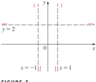
The functionf whose graph is shown in Figure 6 is defined on the closed interval [0, 2]
but has no maximum value. (Notice that the range off is [0, 3). The function takes on val- ues arbitrarily close to 3, but never actually attains the value 3.) This does not contradict the Extreme Value Theorem because f is not continuous. [Nonetheless, a discontinuous function couldhave maximum and minimum values. See Exercise 13(b).]
1
x y
0
F I G U R E 7
This continuous function g has no maximum or minimum.
2 1
x y
0
F I G U R E 6
This function has minimum value f(2)=0, but no maximum value.
2 3
F I G U R E 5 x
y
0 a c d b x
y
0 a c¡ d c™ b x
y
0 a c d=b
关a, b兴 d
c f共d兲
f共c兲 f
关a, b兴 f
3
x苷4
f
f共3兲苷⫺27 f共0兲苷0
f共⫺1兲苷37
f共1兲苷5
⫺1艋 x艋4 f共x兲苷3x4⫺16x3⫹18x2
V
F I G U R E 4 (_1, 37)
_1 1 2 3 4 5
(3, _27) (1, 5)
y
x y=3x$-16˛+18≈
The function tshown in Figure 7 is continuous on the open interval (0, 2) but has nei- ther a maximum nor a minimum value. [The range of tis . The function takes on arbitrarily large values.] This does not contradict the Extreme Value Theorem because the interval (0, 2) is not closed.
The Extreme Value Theorem says that a continuous function on a closed interval has a maximum value and a minimum value, but it does not tell us how to find these extreme values. We start by looking for local extreme values.
Figure 8 shows the graph of a function with a local maximum at and a local minimum at . It appears that at the maximum and minimum points the tangent lines are horizontal and therefore each has slope 0. We know that the derivative is the slope of the tangent line, so it appears that and . The following theorem says that this is always true for differentiable functions.
FERMAT’S THEOREM If has a local maximum or minimum at , and if exists, then .
PROOF Suppose, for the sake of definiteness, that has a local maximum at c. Then, according to Definition 2, if is sufficiently close to . This implies that if
is sufficiently close to 0, with being positive or negative, then
and therefore
We can divide both sides of an inequality by a positive number. Thus, if and is sufficiently small, we have
Taking the right-hand limit of both sides of this inequality (using Theorem 2.3.2), we get
But since exists, we have
and so we have shown that .
If , then the direction of the inequality (5) is reversed when we divide by :
So, taking the left-hand limit, we have
f⬘共c兲苷lim
hl0
f共c⫹h兲⫺f共c兲
h 苷 lim
hl0⫺
f共c⫹h兲⫺f共c兲
h 艌0
h⬍0 f共c⫹h兲⫺f共c兲
h 艌0
h h⬍0
f⬘共c兲艋0 f⬘共c兲苷lim
hl0
f共c⫹h兲⫺f共c兲
h 苷 lim
hl0⫹
f共c⫹h兲⫺f共c兲 h f⬘共c兲
hliml0⫹
f共c⫹h兲⫺f共c兲
h 艋 lim
hl0⫹ 0苷0 f共c⫹h兲⫺f共c兲
h 艋0
h h⬎0 f共c⫹h兲⫺f共c兲艋0
5
f共c兲艌f共c⫹h兲 h
h
c x
f共c兲艌f共x兲
f f⬘共c兲苷0
f⬘共c兲 c
f
4
f⬘共d兲苷0 f⬘共c兲苷0
d
c f
共1, ⬁兲
N Fermat’s Theorem is named after Pierre Fermat (1601–1665), a French lawyer who took up mathematics as a hobby. Despite his amateur status, Fermat was one of the two inventors of analytic geometry (Descartes was the other). His methods for finding tangents to curves and maxi- mum and minimum values (before the invention of limits and derivatives) made him a forerunner of Newton in the creation of differential calculus.
0 c d x
y
{c, f(c)}
{d, f(d)}
F I G U R E 8
We have shown that and also that . Since both of these inequalities must be true, the only possibility is that .
We have proved Fermat’s Theorem for the case of a local maximum. The case of a local minimum can be proved in a similar manner, or we could use Exercise 76 to deduce it from the case we have just proved (see Exercise 77). M
The following examples caution us against reading too much into Fermat’s Theorem.
We can’t expect to locate extreme values simply by setting and solving for .
EXAMPLE 5 If , then , so . But has no maximum or minimum at 0, as you can see from its graph in Figure 9. (Or observe that for
but for .) The fact that simply means that the curve has a horizontal tangent at . Instead of having a maximum or minimum at ,
the curve crosses its horizontal tangent there. M
EXAMPLE 6 The function has its (local and absolute) minimum value at 0, but that value can’t be found by setting because, as was shown in Example 5
in Section 2.8, does not exist. (See Figure 10.) M
| WARNING Examples 5 and 6 show that we must be careful when using Fermat’s Theorem.Example 5 demonstrates thateven when there need not be a maximum or minimum at .(In other words, the converse of Fermat’s Theorem is false in general.) Furthermore, there may be an extreme value even when does not exist (as in Example 6).
Fermat’s Theorem does suggest that we should at least startlooking for extreme values of at the numbers where or where does not exist. Such numbers are given a special name.
DEFINITION A critical numberof a function is a number in the domain of such that either or does not exist.
EXAMPLE 7 Find the critical numbers of . SOLUTION The Product Rule gives
[The same result could be obtained by first writing .] Therefore if , that is, , and does not exist when . Thus the
critical numbers are and . M
In terms of critical numbers, Fermat’s Theorem can be rephrased as follows (compare Definition 6 with Theorem 4):
Iffhas a local maximum or minimum at c, then cis a critical number of f.
7
3 0
2
x苷0 f⬘共x兲
x苷32 12⫺8x苷0
f⬘共x兲苷0
f共x兲苷4x3兾5⫺x8兾5 苷 ⫺5x⫹3共4⫺x兲
5x2兾5 苷 12⫺8x 5x2兾5
f⬘共x兲苷x3兾5共⫺1兲⫹共4⫺x兲
(
35x⫺2兾5)
苷⫺x3兾5⫹ 3共4⫺x兲5x2兾5 f共x兲苷x3兾5共4⫺x兲
V
f⬘共c兲 f⬘共c兲苷0 f
c f
6
f⬘共c兲 f⬘共c兲苷0
c f
f⬘共c兲 c
f⬘共c兲苷0 f⬘共0兲
f⬘共x兲苷0 f共x兲苷
ⱍ
xⱍ
共0, 0兲 共0, 0兲
y苷x3 f⬘共0兲苷0
x⬍0 x3⬍0
x⬎0
x3⬎0 f
f⬘共0兲苷0 f⬘共x兲苷3x2
f共x兲苷x3
x f⬘共x兲苷0
f⬘共c兲苷0 f⬘共c兲艋0 f⬘共c兲艌0
F I G U R E 9
If ƒ=˛, then fª(0)=0 but ƒ has no maximum or minimum.
y=˛
x y
0
F I G U R E 1 0
If ƒ=| x |, then f(0)=0 is a minimum value, but fª(0) does not exist.
0 x
y=|x|
y
F I G U R E 1 1 3.5
_2
_0.5 5
N Figure 11 shows a graph of the function in Example 7. It supports our answer because there is a horizontal tangent when and a vertical tangent when x苷0.
x苷1.5 f
To find an absolute maximum or minimum of a continuous function on a closed interval, we note that either it is local [in which case it occurs at a critical number by (7)] or it occurs at an endpoint of the interval. Thus the following three-step procedure always works.
THE CLOSED INTERVAL METHOD To find the absolutemaximum and minimum values of a continuous function on a closed interval :
1. Find the values of at the critical numbers of in . 2. Find the values of at the endpoints of the interval.
3. The largest of the values from Steps 1 and 2 is the absolute maximum value;
the smallest of these values is the absolute minimum value.
EXAMPLE 8 Find the absolute maximum and minimum values of the function
SOLUTION Since is continuous on , we can use the Closed Interval Method:
Since exists for all , the only critical numbers of occur when , that is, or . Notice that each of these critical numbers lies in the interval . The values of at these critical numbers are
The values of at the endpoints of the interval are
Comparing these four numbers, we see that the absolute maximum value is and the absolute minimum value is .
Note that in this example the absolute maximum occurs at an endpoint, whereas the absolute minimum occurs at a critical number. The graph of is sketched in Figure 12. M
If you have a graphing calculator or a computer with graphing software, it is possible to estimate maximum and minimum values very easily. But, as the next example shows, calculus is needed to find the exactvalues.
EXAMPLE 9
(a) Use a graphing device to estimate the absolute minimum and maximum values of
the function .
(b) Use calculus to find the exact minimum and maximum values.
SOLUTION
(a) Figure 13 shows a graph of in the viewing rectangle by . By mov- ing the cursor close to the maximum point, we see that the -coordinates don’t change very much in the vicinity of the maximum. The absolute maximum value is about 6.97 and it occurs when . Similarly, by moving the cursor close to the minimum point, we see that the absolute minimum value is about ⫺0.68and it occurs when x⬇1.0. It is
x⬇5.2
y
关⫺1, 8兴 关0, 2兴
f
f共x兲苷x⫺2 sin x, 0艋 x艋2
f f共2兲苷⫺3
f共4兲苷17 f共4兲苷17
f
(
⫺12)
苷18f
f共2兲苷⫺3 f共0兲苷1
f
(
⫺12, 4)
x苷2 x苷0
f⬘共x兲苷0 f
x f⬘共x兲
f⬘共x兲苷3x2⫺6x苷3x共x⫺2兲 f共x兲苷x3⫺3x2⫹1
[
⫺12, 4]
f
⫺12艋 x艋4 f共x兲苷x3⫺3x2⫹1
V
f
共a, b兲 f
f
关a, b兴 f
F I G U R E 1 2 5 10 20
_5 15
1 2
3 4
(4, 17)
(2, _3) _1
y=˛-3≈+1
x y
0
F I G U R E 1 3 0
8
_1
2π
possible to get more accurate estimates by zooming in toward the maximum and mini- mum points, but instead let’s use calculus.
(b) The function is continuous on . Since ,
we have when and this occurs when or . The values
of at these critical points are
and
The values of at the endpoints are
Comparing these four numbers and using the Closed Interval Method, we see that the absolute minimum value is and the absolute maximum value is
. The values from part (a) serve as a check on our work. M
EXAMPLE 10 The Hubble Space Telescope was deployed on April 24, 1990, by the space shuttle Discovery.A model for the velocity of the shuttle during this mission, from liftoff at until the solid rocket boosters were jettisoned at , is given by
(in feet per second). Using this model, estimate the absolute maximum and minimum values of theaccelerationof the shuttle between liftoff and the jettisoning of the boosters.
SOLUTION We are asked for the extreme values not of the given velocity function, but rather of the acceleration function. So we first need to differentiate to find the acceleration:
We now apply the Closed Interval Method to the continuous function aon the interval . Its derivative is
The only critical number occurs when :
Evaluating at the critical number and at the endpoints, we have
So the maximum acceleration is about and the minimum acceleration is
about 21.52 ft兾s2. M
62.87 ft兾s2
a共126兲 ⬇62.87 a共t1兲 ⬇21.52
a共0兲苷23.61 a共t兲
t1苷 0.18058
0.007812 ⬇23.12 a⬘共t兲苷0
a⬘共t兲苷0.007812t⫺0.18058 0艋t艋126
苷0.003906t2⫺0.18058t⫹23.61 a共t兲苷v⬘共t兲苷 d
dt 共0.001302t3⫺0.09029t2⫹23.61t⫺3.083兲 v共t兲苷0.001302t3⫺0.09029t2⫹23.61t⫺3.083
t苷126 s t苷0
f共5兾3兲苷5兾3⫹s3
f共兾3兲苷兾3⫺s3
f共2兲苷2⬇6.28 and
f共0兲苷0 f
f共5兾3兲苷 5
3 ⫺2 sin 5 3 苷 5
3 ⫹s3 ⬇6.968039 f共兾3兲苷
3 ⫺2 sin 3 苷
3 ⫺s3 ⬇⫺0.684853 f
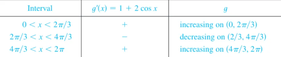
5兾3 x苷兾3
cos x苷12 f⬘共x兲苷0
f⬘共x兲苷1⫺2 cos x 关0, 2兴
f共x兲苷x⫺2 sin x
NASA
(c) Sketch the graph of a function that has a local maximum at 2 and is not continuous at 2.
12. (a) Sketch the graph of a function on [⫺1, 2] that has an absolute maximum but no local maximum.
(b) Sketch the graph of a function on [⫺1, 2] that has a local maximum but no absolute maximum.
(a) Sketch the graph of a function on [⫺1, 2] that has an absolute maximum but no absolute minimum.
(b) Sketch the graph of a function on [⫺1, 2] that is discontin- uous but has both an absolute maximum and an absolute minimum.
14. (a) Sketch the graph of a function that has two local maxima, one local minimum, and no absolute minimum.
(b) Sketch the graph of a function that has three local minima, two local maxima, and seven critical numbers.
15 – 28 Sketch the graph of by hand and use your sketch to find the absolute and local maximum and minimum values of . (Use the graphs and transformations of Sections 1.2 and 1.3.)
15. ,
16. ,
17. ,
18. ,
19. ,
20. ,
21. ,
22. ,
23. ,
24. ,
26.
27.
28.
29 – 44 Find the critical numbers of the function.
29. 30.
31. 32.
33. 34.
35. 36. h共p兲苷 p⫺1
p2⫹4 t共y兲苷 y⫺1
y2⫺y⫹1
t共t兲苷
ⱍ
3t⫺4ⱍ
s共t兲苷3t4⫹4t3⫺6t2
f共x兲苷x3⫹x2⫹x f共x兲苷x3⫹3x2⫺24x
f共x兲苷x3⫹x2⫺x f共x兲苷5x2⫹4x
f共x兲苷
再
42x⫺⫺x21if ⫺2艋x⬍0 if 0艋x艋2 f共x兲苷
再
12x⫺⫺x4if 0艋x⬍2 if 2艋x艋3 f共x兲苷ex
f共x兲苷1⫺sx 25.
⫺3兾2艋t艋3兾2 f共t兲苷cos t
0⬍x艋2 f共x兲苷ln x
⫺2艋x⬍5 f共x兲苷1⫹共x⫹1兲2
⫺3艋x艋2 f共x兲苷x2
0艋x艋2 f共x兲苷x2
0艋x⬍2 f共x兲苷x2
0⬍x艋2 f共x兲苷x2
0⬍x⬍2 f共x兲苷x2
x艋5 f共x兲苷3⫺2x
x艌1 f共x兲苷8⫺3x
f f
13.
1. Explain the difference between an absolute minimum and a local minimum.
2. Suppose is a continuous function defined on a closed interval .
(a) What theorem guarantees the existence of an absolute max- imum value and an absolute minimum value for ? (b) What steps would you take to find those maximum and
minimum values?
3 – 4 For each of the numbers a, b, c, d, r, and s, state whether the function whose graph is shown has an absolute maximum or min- imum, a local maximum or minimum, or neither a maximum nor a minimum.
3. 4.
5 – 6 Use the graph to state the absolute and local maximum and minimum values of the function.
5. 6.
7–10 Sketch the graph of a function that is continuous on [1, 5] and has the given properties.
7. Absolute minimum at 2, absolute maximum at 3, local minimum at 4
8. Absolute minimum at 1, absolute maximum at 5, local maximum at 2, local minimum at 4 Absolute maximum at 5, absolute minimum at 2, local maximum at 3, local minima at 2 and 4
10. has no local maximum or minimum, but 2 and 4 are critical numbers
(a) Sketch the graph of a function that has a local maximum at 2 and is differentiable at 2.
(b) Sketch the graph of a function that has a local maximum at 2 and is continuous but not differentiable at 2.
11.
f 9.
f y
0 x
y=©
1 1 y
0 x
1 y=ƒ
1
x y
0 a b c d r s
x y
0 a b c d r s
f 关a, b兴
f
E X E R C I S E S
4.1
68.
69. Between and , the volume (in cubic centimeters) of 1 kg of water at a temperature is given approximately by the formula
Find the temperature at which water has its maximum density.
70. An object with weight is dragged along a horizontal plane by a force acting along a rope attached to the object. If the rope makes an angle with the plane, then the magnitude of the force is
where is a positive constant called the coefficient of friction and where . Show that is minimized when
.
71. A model for the US average price of a pound of white sugar from 1993 to 2003 is given by the function
where is measured in years since August of 1993. Estimate the times when sugar was cheapest and most expensive dur- ing the period 1993–2003.
;72. On May 7, 1992, the space shuttle Endeavourwas launched on mission STS-49, the purpose of which was to install a new perigee kick motor in an Intelsat communications satellite.
The table gives the velocity data for the shuttle between liftoff and the jettisoning of the solid rocket boosters.
(a) Use a graphing calculator or computer to find the cubic polynomial that best models the velocity of the shuttle for the time interval . Then graph this polynomial.
(b) Find a model for the acceleration of the shuttle and use it to estimate the maximum and minimum values of the acceleration during the first 125 seconds.
t僆关0, 125兴 t
⫹0.03629t2⫺0.04458t⫹0.4074 S共t兲苷⫺0.00003237t5⫹0.0009037t4⫺0.008956t3 tan 苷
F 0艋 艋 兾2
F苷 W
sin ⫹cos
W
V苷999.87⫺0.06426T⫹0.0085043T2⫺0.0000679T3 T
30⬚C V 0⬚C
f共x兲苷x⫺2 cos x, ⫺2艋x艋0 f共x兲苷xsx⫺x2
37. 38. 67.
40.
42.
43. 44.
;45 – 46 A formula for the derivativeof a function is given. How many critical numbers does have?
45. 46.
47– 62 Find the absolute maximum and absolute minimum values of on the given interval.
47. ,
48. ,
,
50. ,
51. ,
52. ,
53. ,
54. ,
55. ,
56. ,
57. ,
58. ,
59. ,
60. ,
61.
62.
63. If and are positive numbers, find the maximum value
of , .
;64. Use a graph to estimate the critical numbers of correct to one decimal place.
;65 – 68
(a) Use a graph to estimate the absolute maximum and minimum values of the function to two decimal places.
(b) Use calculus to find the exact maximum and minimum values.
65.
66. f共x兲苷ex3⫺x, ⫺1艋x艋0 f共x兲苷x5⫺x3⫹2, ⫺1艋x艋1 f共x兲苷
ⱍ
x3⫺3x2⫹2ⱍ
0艋x艋1 f共x兲苷xa共1⫺x兲b
b a
f共x兲苷e⫺x⫺e⫺2x, 关0, 1兴 f共x兲苷ln共x2⫹x⫹1兲, 关⫺1, 1兴
[
12, 2]
f共x兲苷x⫺ln x 关⫺1, 4兴 f共x兲苷xe⫺x2兾8
关兾4, 7兾4兴 f共t兲苷t⫹cot共t兾2兲
关0,兾2兴 f共t兲苷2 cos t⫹sin 2t
关0, 8兴 f共t兲苷s3t共8⫺t兲
关⫺1, 2兴 f共t兲苷ts4⫺t2
关⫺4, 4兴 f共x兲苷 x2⫺4
x2⫹4 关0, 2兴 f共x兲苷 x
x2⫹1
关⫺1, 2兴 f共x兲苷共x2⫺1兲3
关⫺2, 3兴 f共x兲苷x4⫺2x2⫹3
关⫺1, 4兴 f共x兲苷x3⫺6x2⫹9x⫹2
关⫺2, 3兴 f共x兲苷2x3⫺3x2⫺12x⫹1
49.
关0, 3兴 f共x兲苷x3⫺3x⫹1
关0, 3兴 f共x兲苷3x2⫺12x⫹5 f
f⬘共x兲苷 100 cos2x 10⫹x2 ⫺1 f⬘共x兲苷5e⫺0.1 ⱍxⱍsinx⫺1
f
f f共x兲苷x⫺2 ln x f共x兲苷x2e⫺3x
t共兲苷4 ⫺tan f共兲苷2 cos ⫹sin2
41.
t共x兲苷x1兾3⫺x⫺2兾3 F共x兲苷x4兾5共x⫺4兲2
39.
t共x兲苷s1⫺x2 h共t兲苷t3兾4⫺2t1兾4
Event Time (s) Velocity (ft兾s)
Launch 0 0
Begin roll maneuver 10 185
End roll maneuver 15 319
Throttle to 89% 20 447
Throttle to 67% 32 742
Throttle to 104% 59 1325
Maximum dynamic pressure 62 1445
Solid rocket booster separation 125 4151
(b) What is the absolute maximum value of on the interval?
(c) Sketch the graph of on the interval . 74. Show that 5 is a critical number of the function
but does not have a local extreme value at 5.
75. Prove that the function
has neither a local maximum nor a local minimum.
76. If has a minimum value at , show that the function has a maximum value at .
77. Prove Fermat’s Theorem for the case in which has a local minimum at .
A cubic function is a polynomial of degree 3; that is, it has the
form , where .
(a) Show that a cubic function can have two, one, or no critical number(s). Give examples and sketches to illustrate the three possibilities.
(b) How many local extreme values can a cubic function have?
a苷0 f共x兲苷ax3⫹bx2⫹cx⫹d
78.
c
f t共x兲苷⫺f共x兲 c
c f
f共x兲苷x101⫹x51⫹x⫹1 t
t共x兲苷2⫹共x⫺5兲3 关0, r0兴 v
73. When a foreign object lodged in the trachea (windpipe) forces v a person to cough, the diaphragm thrusts upward causing an increase in pressure in the lungs. This is accompanied by a contraction of the trachea, making a narrower channel for the expelled air to flow through. For a given amount of air to escape in a fixed time, it must move faster through the narrower channel than the wider one. The greater the velocity of the airstream, the greater the force on the foreign object.
X rays show that the radius of the circular tracheal tube contracts to about two-thirds of its normal radius during a cough. According to a mathematical model of coughing, the velocity of the airstream is related to the radius of the trachea by the equation
where is a constant and is the normal radius of the trachea.
The restriction on is due to the fact that the tracheal wall stiff- ens under pressure and a contraction greater than is prevented (otherwise the person would suffocate).
(a) Determine the value of in the interval at which has an absolute maximum. How does this compare with experimental evidence?
[
12r0, r0]
v r1 2r0
r r0
k
1
2r0艋r艋r0
v共r兲苷k共r0⫺r兲r2
r v
Rainbows are created when raindrops scatter sunlight. They have fascinated mankind since ancient times and have inspired attempts at scientific explanation since the time of Aristotle. In this project we use the ideas of Descartes and Newton to explain the shape, location, and colors of rainbows.
1. The figure shows a ray of sunlight entering a spherical raindrop at . Some of the light is reflected, but the line shows the path of the part that enters the drop. Notice that the light is refracted toward the normal line and in fact Snell’s Law says that , where is the angle of incidence, is the angle of refraction, and is the index of refraction for water. At some of the light passes through the drop and is refracted into the air, but the line shows the part that is reflected. (The angle of incidence equals the angle of reflection.) When the ray reaches , part of it is reflected, but for the time being we are more interested in the part that leaves the raindrop at . (Notice that it is refracted away from the normal line.) The angle of deviation is the amount of clockwise rotation that the ray has undergone during this three-stage process. Thus
Show that the minimum value of the deviation is and occurs when . The significance of the minimum deviation is that when we have , so
. This means that many rays with become deviated by approximately the same amount. It is the concentrationof rays coming from near the direction of minimum deviation that creates the brightness of the primary rainbow. The figure at the left shows that the angle of elevation from the observer up to the highest point on the rainbow is
. (This angle is called the rainbow angle.)
2. Problem 1 explains the location of the primary rainbow, but how do we explain the colors?
Sunlight comprises a range of wavelengths, from the red range through orange, yellow, 180⬚ ⫺138⬚苷42⬚
␣⬇59.4⬚
⌬D兾⌬␣⬇0
D⬘共␣兲 ⬇0
␣⬇59.4⬚
␣⬇59.4⬚
D共␣兲 ⬇138⬚
D共␣兲苷共␣ ⫺ 兲⫹共 ⫺2兲⫹共␣ ⫺ 兲苷 ⫹2␣ ⫺4
D共␣兲 C C
BC B
k⬇43

␣
sin ␣苷k sin  AO
AB
A THE C ALCULUS OF RAINBOWS
A P P L I E D P R O J E C T
å
å
D(å )
∫ A fromsun
Formation of the primary rainbow to
observer C
B O
∫∫
∫
rays from sun rays from sun
42°
138°
observer
green, blue, indigo, and violet. As Newton discovered in his prism experiments of 1666, the index of refraction is different for each color. (The effect is called dispersion.) For red light the refractive index is whereas for violet light it is . By repeating the calculation of Problem 1 for these values of , show that the rainbow angle is about for the red bow and for the violet bow. So the rainbow really consists of seven individual bows corresponding to the seven colors.
3. Perhaps you have seen a fainter secondary rainbow above the primary bow. That results from the part of a ray that enters a raindrop and is refracted at , reflected twice (at and ), and refracted as it leaves the drop at (see the figure). This time the deviation angle is the total amount of counterclockwise rotation that the ray undergoes in this four-stage process.
Show that
and has a minimum value when
Taking , show that the minimum deviation is about and so the rainbow angle for the secondary rainbow is about , as shown in the figure.
4. Show that the colors in the secondary rainbow appear in the opposite order from those in the primary rainbow.
42° 51°
51⬚
129⬚
k苷43
cos ␣苷
冑
k2⫺8 1D共␣兲
D共␣兲苷2␣ ⫺6 ⫹2
D共␣兲 D
C B A
40.6⬚
42.3⬚
k
k⬇1.3435 k⬇1.3318
Formation of the secondary rainbow D
C
B A
å
å
∫ ∫
∫
∫ ∫
∫ to
observer
from sun
T H E M E A N VA L U E T H E O R E M
We will see that many of the results of this chapter depend on one central fact, which is called the Mean Value Theorem. But to arrive at the Mean Value Theorem we first need the following result.
ROLLE’S THEOREM Let be a function that satisfies the following three hypotheses:
1. is continuous on the closed interval . 2. is differentiable on the open interval . 3.
Then there is a number in c 共a, b兲such that f⬘共c兲苷0. f共a兲苷f共b兲
共a, b兲 f
关a, b兴 f
f
4.2
N Rolle’s Theorem was first published in 1691 by the French mathematician Michel Rolle (1652–1719) in a book entitled Méthode pour résoudre les égalitéz. He was a vocal critic of the methods of his day and attacked calculus as being a “collection of ingenious fallacies.” Later, however, he became convinced of the essential correctness of the methods of calculus.
© C. Donald Ahrens
Before giving the proof let’s take a look at the graphs of some typical functions that sat- isfy the three hypotheses. Figure 1 shows the graphs of four such functions. In each case it appears that there is at least one point on the graph where the tangent is hori- zontal and therefore . Thus Rolle’s Theorem is plausible.
PROOF There are three cases:
CASE I N , a constant
Then , so the number can be taken to be anynumber in . CASE II N for some xin [as in Figure 1(b) or (c)]
By the Extreme Value Theorem (which we can apply by hypothesis 1), has a maxi- mum value somewhere in . Since , it must attain this maximum value at a number in the open interval . Then has a localmaximum at and, by hypoth- esis 2, is differentiable at . Therefore by Fermat’s Theorem.
CASE III N for some xin [as in Figure 1(c) or (d)]
By the Extreme Value Theorem, has a minimum value in and, since , it attains this minimum value at a number in . Again by Fermat’s
Theorem. M
EXAMPLE 1 Let’s apply Rolle’s Theorem to the position function of a moving object. If the object is in the same place at two different instants and , then
. Rolle’s Theorem says that there is some instant of time between and when ; that is, the velocity is 0. (In particular, you can see that this is true
when a ball is thrown directly upward.) M
EXAMPLE 2 Prove that the equation has exactly one real root.
SOLUTION First we use the Intermediate Value Theorem (2.5.10) to show that a root exists.
Let . Then and . Since is a polynomi-
al, it is continuous, so the Intermediate Value Theorem states that there is a number between 0 and 1 such that . Thus the given equation has a root.
To show that the equation has no other real root, we use Rolle’s Theorem and argue by contradiction. Suppose that it had two roots and . Then and, since is a polynomial, it is differentiable on and continuous on . Thus, by Rolle’s Theorem, there is a number between and such that . But
(since ) so can never be 0. This gives a contradiction. Therefore the equation
can’t have two real roots. M
f⬘共x兲 x2艌0
for all x f⬘共x兲苷3x2⫹1艌1
f⬘共c兲苷0 b
a c
关a, b兴 共a, b兲
f f共a兲苷0苷f共b兲
b a f共c兲苷0
c f
f共1兲苷1⬎0 f共0兲苷⫺1⬍0
f共x兲苷x3⫹x⫺1
x3⫹x⫺1苷0 f⬘共c兲苷0
b
a t苷c
f共a兲苷f共b兲
t苷b t苷a
s苷f共t兲 f⬘共c兲苷0 共a, b兲
c
f共a兲苷f共b兲 关a, b兴
f
共a, b兲 f共x兲⬍f共a兲
f⬘共c兲苷0 c
f
c 共a, b兲 f
c
f共a兲苷f共b兲 关a, b兴
f 共a, b兲
f共x兲⬎f共a兲
共a, b兲 c
f⬘共x兲苷0 f共x兲苷k F I G U R E 1
(a)
b
a c¡ c™ x
y
0
(b)
a c b x
y
0
(c)
b
a c¡ c™ x
y
0
(d) b
a c
y
0 x
f⬘共c兲苷0
共c, f共c兲兲
NTake cases
N Figure 2 shows a graph of the function discussed in Example 2.
Rolle’s Theorem shows that, no matter how much we enlarge the viewing rectangle, we can never find a second -intercept.x
f共x兲苷x3⫹x⫺1
F I G U R E 2 _2
3
_3
2
Our main use of Rolle’s Theorem is in proving the following important theorem, which was first stated by another French mathematician, Joseph-Louis Lagrange.
THE MEAN VALUE THEOREM Let be a function that satisfies the following hypotheses:
1. is continuous on the closed interval . 2. is differentiable on the open interval . Then there is a number in such that
or, equivalently,
Before proving this theorem, we can see that it is reasonable by interpreting it geomet- rically. Figures 3 and 4 show the points and on the graphs of two dif- ferentiable functions. The slope of the secant line is
which is the same expression as on the right side of Equation 1. Since is the slope of the tangent line at the point , the Mean Value Theorem, in the form given by Equa- tion 1, says that there is at least one point on the graph where the slope of the tangent line is the same as the slope of the secant line . In other words, there is a point
where the tangent line is parallel to the secant line .
PROOF We apply Rolle’s Theorem to a new function defined as the difference between and the function whose graph is the secant line . Using Equation 3, we see that the equation of the line can be written as
or as y苷f共a兲⫹ f共b兲⫺f共a兲
b⫺a 共x⫺a兲 y⫺f共a兲苷 f共b兲⫺f共a兲
b⫺a 共x⫺a兲 AB
AB f
h
F I G U R E 3 F I G U R E 4
0 x
y
a c b
B{b, f(b)}
P{c, f(c)}
A{a, f(a)}
0 x
y
c¡ c™
P¡ B
A P™
b a
AB P
AB P共c, f共c兲兲 共c, f共c兲兲
f⬘共c兲 mAB苷 f共b兲⫺f共a兲
b⫺a
3
AB
B共b, f共b兲兲 A共a, f共a兲兲
f共b兲⫺f共a兲苷f⬘共c兲共b⫺a兲
2
f⬘共c兲苷 f共b兲⫺f共a兲 b⫺a
1
共a, b兲 c
共a, b兲 f
关a, b兴 f
f
N The Mean Value Theorem is an example of what is called an existence theorem. Like the Intermediate Value Theorem, the Extreme Value Theorem, and Rolle’s Theorem, it guarantees that there existsa number with a certain property, but it doesn’t tell us how to find the number.
So, as shown in Figure 5,
First we must verify that satisfies the three hypotheses of Rolle’s Theorem.
1. The function is continuous on because it is the sum of and a first-degree polynomial, both of which are continuous.
2. The function is differentiable on because both and the first-degree poly- nomial are differentiable. In fact, we can compute directly from Equation 4:
(Note that and are constants.)
3.
Therefore, .
Since satisfies the hypotheses of Rolle’s Theorem, that theorem says there is a num- ber in such that . Therefore
and so M
EXAMPLE 3 To illustrate the Mean Value Theorem with a specific function, let’s con- sider . Since is a polynomial, it is continuous and differ- entiable for all , so it is certainly continuous on and differentiable on . Therefore, by the Mean Value Theorem, there is a number in such that
Now , and , so this equation becomes
which gives , that is, . But must lie in , so .
Figure 6 illustrates this calculation: The tangent line at this value of is parallel to the
secant line . M
EXAMPLE 4 If an object moves in a straight line with position function , then the average velocity between and is
f共b兲⫺f共a兲 b⫺a t苷b t苷a
s苷f共t兲
V
OB
c
c苷2兾s3 共0, 2兲
c c苷⫾2兾s3 c2苷43
6苷共3c2⫺1兲2苷6c2⫺2 f⬘共x兲苷3x2⫺1
f共2兲苷6, f共0兲苷0
f共2兲⫺f共0兲苷f⬘共c兲共2⫺0兲
共0, 2兲 c
共0, 2兲 关0, 2兴
x
f f共x兲苷x3⫺x, a苷0, b苷2
V
f⬘共c兲苷 f共b兲⫺f共a兲 b⫺a
0苷h⬘共c兲苷f⬘共c兲⫺ f共b兲⫺f共a兲 b⫺a h⬘共c兲苷0
共a, b兲 c
h
h共a兲苷h共b兲
苷f共b兲⫺f共a兲⫺关f共b兲⫺f共a兲兴苷0 h共b兲苷f共b兲⫺f共a兲⫺ f共b兲⫺f共a兲
b⫺a 共b⫺a兲 h共a兲苷f共a兲⫺f共a兲⫺ f共b兲⫺f共a兲
b⫺a 共a⫺a兲苷0 关f共b兲⫺f共a兲兴兾共b⫺a兲
f共a兲
h⬘共x兲苷f⬘共x兲⫺ f共b兲⫺f共a兲 b⫺a
h⬘
共a, b兲 f h
关a, b兴 f h
h
h共x兲苷f共x兲⫺f共a兲⫺ f共b兲⫺f共a兲
b⫺a 共x⫺a兲
4
F I G U R E 5
0 x
y
x
h(x) y=ƒ
ƒ A
B
f(a)+f(b)-f(a)(x-a) b-a
The Mean Value Theorem was first formulated by Joseph-Louis Lagrange (1736–1813), born in Italy of a French father and an Italian mother. He was a child prodigy and became a professor in Turin at the tender age of 19. Lagrange made great con- tributions to number theory, theory of functions, theory of equations, and analytical and celestial mechanics. In particular, he applied calculus to the analysis of the stability of the solar system. At the invitation of Frederick the Great, he succeeded Euler at the Berlin Academy and, when Frederick died, Lagrange accepted King Louis XVI’s invitation to Paris, where he was given apartments in the Louvre and became a professor at the Ecole Poly- technique. Despite all the trappings of luxury and fame, he was a kind and quiet man, living only for science.
LAGRANGE AND THE MEAN VALUE THEOREM
F I G U R E 6
y=˛- x B
x y
c 2
O
and the velocity at is . Thus the Mean Value Theorem (in the form of Equa- tion 1) tells us that at some time between and the instantaneous velocity is equal to that average velocity. For instance, if a car traveled 180 km in 2 hours, then the speedometer must have read 90 km兾h at least once.
In general, the Mean Value Theorem can be interpreted as saying that there is a num- ber at which the instantaneous rate of change is equal to the average rate of change over
an interval. M
The main significance of the Mean Value Theorem is that it enables us to obtain infor- mation about a function from information about its derivative. The next example provides an instance of this principle.
EXAMPLE 5 Suppose that and for all values of . How large can possibly be?
SOLUTION We are given that is differentiable (and therefore continuous) everywhere.
In particular, we can apply the Mean Value Theorem on the interval . There exists a number such that
so
We are given that for all , so in particular we know that . Multiply- ing both sides of this inequality by 2, we have , so
The largest possible value for is 7. M
The Mean Value Theorem can be used to establish some of the basic facts of differen- tial calculus. One of these basic facts is the following theorem. Others will be found in the following sections.
THEOREM If for all in an interval , then is constant on .
PROOF Let and be any two numbers in with . Since is differen- tiable on , it must be differentiable on and continuous on . By apply- ing the Mean Value Theorem to on the interval , we get a number such that
and
Since for all , we have , and so Equation 6 becomes
Therefore has the same value at anytwo numbers and in . This means that
is constant on . M
COROLLARY If for all in an interval , then is con- stant on 共a, b兲; that is, f共x兲苷t共x兲⫹cwhere is a constant.c
f⫺t 共a, b兲
x f⬘共x兲苷t⬘共x兲
7
共a, b兲
共a, b兲 f x2
x1
f
f共x2兲苷f共x1兲 or
f共x2兲⫺f共x1兲苷0 f⬘共c兲苷0 x
f⬘共x兲苷0
f共x2兲⫺f共x1兲苷f⬘共c兲共x2⫺x1兲
6
x1⬍c⬍x2
关x1, x2兴 c f
关x1, x2兴 共x1, x2兲
共a, b兲
f x1⬍x2
共a, b兲 x2
x1
共a, b兲 共a, b兲 f
x f⬘共x兲苷0
5
f共2兲
f共2兲苷⫺3⫹2f⬘共c兲艋 ⫺3⫹10苷7 2f⬘共c兲艋10
f⬘共c兲艋5 x
f⬘共x兲艋5
f共2兲苷f共0兲⫹2f⬘共c兲苷⫺3⫹2f⬘共c兲 f共2兲⫺f共0兲苷f⬘共c兲共2⫺0兲 c
关0, 2兴 f
f共2兲
x f⬘共x兲艋5
f共0兲苷⫺3
V
f⬘共c兲 b
a t苷c
f⬘共c兲 t苷c
PROOF Let . Then
for all in . Thus, by Theorem 5, is constant; that is, is constant. M Care must be taken in applying Theorem 5. Let
The domain of is and for all in . But is obviously not a constant function. This does not contradict Theorem 5 because is not an interval. Notice that is constant on the interval and also on the interval .
EXAMPLE 6 Prove the identity .
SOLUTION Although calculus isn’t needed to prove this identity, the proof using calculus is
quite simple. If , then
for all values of . Therefore , a constant. To determine the value of , we put [because we can evaluate exactly]. Then
Thus tan⫺1x⫹cot⫺1x苷兾2. M
C苷f共1兲苷tan⫺1 1⫹cot⫺1 1苷 4 ⫹
4 苷 2 f共1兲
x苷1
C f共x兲苷C
x
f⬘共x兲苷 1
1⫹x2 ⫺ 1 1⫹x2 苷0 f共x兲苷tan⫺1x⫹cot⫺1x
tan⫺1x⫹cot⫺1x苷兾2
共⫺⬁, 0兲 共0, ⬁兲
f
D f D x f⬘共x兲苷0
D苷兵x
ⱍ
x苷0其f
f共x兲苷 x
ⱍ
xⱍ
苷再
1⫺1if x⬎0 if x⬍0 N OT E
f⫺t 共a, b兲 F
x
F⬘共x兲苷f⬘共x兲⫺t⬘共x兲苷0 F共x兲苷f共x兲⫺t共x兲
7. Use the graph of to estimate the values of that satisfy the conclusion of the Mean Value Theorem for the interval .
8. Use the graph of given in Exercise 7 to estimate the values of that satisfy the conclusion of the Mean Value Theorem for the interval 关1, 7兴.
c
f y
y =ƒ
1
x
0 1
关0, 8兴 c
f 1– 4 Verify that the function satisfies the three hypotheses of
Rolle’s Theorem on the given interval. Then find all numbers that satisfy the conclusion of Rolle’s Theorem.
1.
2.
3.
4.
Let . Show that but there is no
number in such that . Why does this not contradict Rolle’s Theorem?
6. Let . Show that but there is no
number in such that . Why does this not contradict Rolle’s Theorem?
f⬘共c兲苷0 共0, 兲
c
f共0兲苷f共兲 f共x兲苷tan x
f⬘共c兲苷0 共⫺1, 1兲
c
f共⫺1兲苷f共1兲 f共x兲苷1⫺x2兾3
5.
关兾8, 7兾8兴 f共x兲苷cos 2x,
关0, 9兴 f共x兲苷sx ⫺13x,
关0, 3兴 f共x兲苷x3⫺x2⫺6x⫹2,
关1, 3兴 f共x兲苷5⫺12x⫹3x2,
c E X E R C I S E S