A Novel Discrete Wavelet Transform Framework for Full Reference Image Quality Assessment

A Novel Discrete Wavelet Transform Framework for Full Reference Image Quality Assessment

Soroosh Rezazadeh, Stéphane Coulombe

Department of Software and IT Engineering, École de technologie supérieure, Université du Québec Montréal, Québec, H3C 1K3, Canada

E-mail: [email protected], [email protected]

Abstract

In this paper, we present a general framework for computing full reference image quality scores in the discrete wavelet domain using the Haar wavelet. In our framework, quality metrics are categorized as either map-based, which generate a quality (distortion) map to be pooled for the final score, e.g. structural similarity (SSIM), or non map-based, which only give a final score, e.g. PSNR. For map-based metrics, the proposed framework defines a contrast map in the wavelet domain for pooling the quality maps. We also derive a formula to enable the framework to automatically calculate the appropriate level of wavelet decomposition for error-based metrics at a desired viewing distance. To consider the effect of very fine image details in quality assessment, the proposed method defines a multi-level edge map for each image, which comprises only the most informative image subbands.

To clarify the application of the framework in computing quality scores, we give some examples to show how the framework can be applied to improve well-known metrics such as SSIM, visual information fidelity (VIF), PSNR, and absolute difference (AD). The proposed framework presents an excellent tradeoff between accuracy and complexity. We compare the complexity of various algorithms obtained by the framework to H.264 encoding based on C/C++ implementations. For example, by using the framework, we can compute the VIF at about 5% of the complexity of its original version, but with higher accuracy.

Accepted in Signal, Image and Video processing (Springer), 2013

The final publication is available at http://link.springer.com/article/10.1007%2Fs11760-011-0260-6

I. INTRODUCTION

Image quality assessment plays an important role in the development and validation of various image and video applications, such as compression and enhancement. Objective quality models are usually classified based on the availability of reference images. If an undistorted reference image is available, the quality metric is considered as a full reference (FR) assessment method. The peak signal-to-noise ratio (PSNR) is the oldest and most widely used FR image quality evaluation measure, because it is simple, has clear physical meaning, is parameter-free, and performs superbly in an optimization context) [1].

However, conventional PSNR cannot adequately reflect the human perception of image fidelity, that is, a large PSNR gain may result in a small improvement in visual quality. This has led researchers to develop a number of other quality measures. Generally speaking, the FR quality assessment of image signals involves two categories of approach: bottom-up and top-down [2].

In the bottom-up approaches, perceptual quality scores are best estimated by quantifying the visibility of errors. In order to quantize errors according to human visual system (HVS) features, techniques in this category try to model the functional properties of different stages of the HVS as characterized by both psychophysical and physiological experiments. This is usually accomplished in several stages of preprocessing, frequency analysis, contrast sensitivity, luminance masking, contrast masking, and error pooling [2],[3]. Most HVS-based quality assessment techniques are multi-channel models, in which each band of spatial frequencies is dealt with by an independent channel. In the Teo and Heeger metric, the steerable pyramid transform is used to decompose the image into several spatial frequency levels, where each level is further divided into a set of six orientation bands [4]. The VSNR [5] is another advanced HVS-based metric, which, after preprocessing, decomposes both the reference image and the errors between the reference and distorted images into five levels, using the discrete wavelet transform and the 9/7 biorthogonal filters. It then computes the contrast detection threshold to assess the detectability of the distortions for each subband of the wavelet decomposition. Some other well-known methods in this category that exploit the Fourier transform rather than multi-resolution decomposition are wSNR, NQM

[6], and PQS [7]. The bottom-up approaches have several limitations, the most important of which is the complexity of HVS models and their non linearities [2], [8].

In the top-down techniques, the overall functionality of the HVS is considered as a black box, and it is the input/output relationship that is of interest. Two main strategies applied in this category are the structural approach and the information-theoretic approach.

Perhaps the most important method of the structural approach is the Structural SIMilarity (SSIM) index [8], which gives an accurate score with acceptable computational complexity compared with other quality metrics [9]. SSIM has attracted a great deal of attention in recent years, and has been considered for a wide range of applications. There have been attempts made to improve the SSIM index. With a view to increasing SSIM assessment accuracy, multi-scale SSIM [10] incorporates image details at five different resolutions with the application of successive low pass filtering and downsampling. In [11], the authors investigate ways to simplify SSIM in the pixel domain. The authors in [12] propose to compute SSIM using subbands at different levels in the discrete wavelet domain. Five-level decomposition using the Daubechies 9/7 wavelet is applied to both the original and the distorted images, and then SSIMs are computed between corresponding subbands. Finally, the similarity score is obtained by the weighted sum of all mean SSIMs. To determine the weights, a large number of experiments have been performed to measure the sensitivity of the human eye to different frequency bands. CW-SSIM, which is presented in [13],[14], benefits from a complex version of 6-scale, 16-orientation steerable pyramid decomposition characteristics to propose a metric resistant to small geometrical distortions.

In the information-theoretic approach, visual quality assessment is viewed as an information fidelity problem. An information fidelity criterion (IFC) for image quality measurement is presented in [15], which works based on natural scene statistics. In the IFC, the image source is modeled using a Gaussian scale mixture (GSM), while the image distortion process is modeled as an error-prone communication channel. The information shared between the images being compared is quantified using the mutual information that is a statistical measure of information fidelity. Another information-theoretic quality metric is the Visual Information Fidelity (VIF) index [16]. This index follows the same procedure as the

IFC, except that, in the VIF, both the image distortion process and the visual perception process are modeled as error-prone communication channels. The VIF index is the most accurate image quality metric, according to the performance evaluation of the prominent image quality assessment algorithms presented in [9].

In this paper, we propose a novel general framework to calculate image quality metrics (IQM) in the discrete wavelet domain. The proposed framework can be applied to both structural (top-down) and error- based (bottom-up) approaches, as explained in subsequent sections. This framework can be applied to map-based metrics, which generate quality (or distortion) maps such as the SSIM map and the absolute difference (AD) map, or to non map-based ones, which give a final score such as the PSNR and the VIF index. We also show that, for these metrics, the framework leads to improved accuracy and reduced complexity compared to the original metrics.

We developed the new framework mainly because of the following shortcomings of the current methods. First, the computational complexity of assessment techniques that accurately predict quality scores is very high. Some image/video processing problems, like identifying the best quantization parameters in image or video encoding [17], can be solved more efficiently if an accurate low complexity quality metric is used. Second, the bottom-up approach reviewed [4],[5] specifies that those techniques apply the multi-resolution transform, decomposing the input image into large numbers of resolutions (five or more). As the HVS is a complex system that is not completely known to us, combining the various bands into the final metric is difficult. In similar top-down methods, such as multi-scale and multi-level SSIMs [10], [12], determining the sensitivity of the HVS to different scales or subbands requires many experiments. Our new approach does not require such heavy experimentation to determine parameters.

Third, top-down methods, like SSIM, gather local statistics within a square sliding window, and the computed statistics of image blocks in the wavelet domain are more accurate. Fourth, a large number of decomposition levels, as in [12], would make the size of the approximation subband very small, so it would no longer be able to help in extracting image statistics effectively. In contrast, the approximation subband contains the main image content, and we have observed that this subband has a major impact on

improving quality prediction accuracy. Fifth, previous SSIM methods use the mean of the quality map to give the overall image quality score. However, distortions in various image areas have different impacts on the HVS. In our framework, we introduce a contrast map in the wavelet domain for pooling quality maps.

The rest of paper is organized as follows. In section 2, we describe the proposed general framework for image quality assessment. In section 3, we explain how the proposed framework is used to calculate the currently well-known objective quality metrics. In section 4, the experimental results are presented.

Finally, our concluding remarks are given in section 5.

II. THE PROPOSED DISCRETE WAVELET DOMAIN IMAGE QUALITY ASSESSMENT

FRAMEWORK

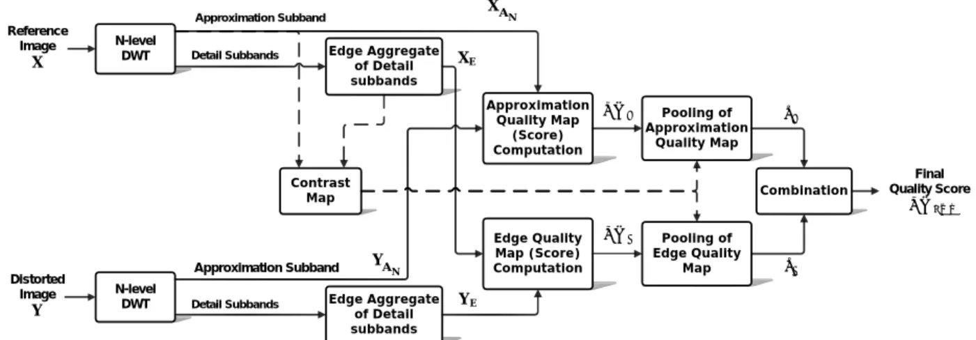
In this section, we describe a DWT-based framework for computing a general purpose FR image quality metric (IQM). The block diagram of the proposed framework is shown in Fig. 1. The dashed lines in this figure display the parts that may be omitted based on whether or not it is a map-based metric. Let X and Y denote the reference and distorted images respectively. The procedure for calculating the proposed version of IQM is set out and explained in the following steps.

Contrast Map

Edge Aggregate of Detail subbands

Edge Aggregate of Detail subbands

Approximation Quality Map

(Score) Computation

Edge Quality Map (Score) Computation

Pooling of Approximation

Quality Map

Pooling of Edge Quality

Map IQMA

IQME

Combination SA

SE N-level

DWT Detail Subbands Reference

Image X

N-level

DWT Detail Subbands Approximation Subband

Distorted Image

Y YE

Approximation Subband

XE

Final Quality Score

IQMDWT AN

X

AN

Y

Fig. 1. Block diagram of the proposed discrete wavelet domain image quality assessment framework

Step 1. We perform N-level DWT on both the reference and the distorted images based on the Haar wavelet filter. With N-level decomposition, the approximation subbands

AN

X and

AN

Y , as well as a number of detail subbands, are obtained.

The Haar wavelet has been used previously in some quality assessment and compression methods [18],[19]. For our framework, we chose the Haar filter for its simplicity and good performance. The Haar wavelet has very low computational complexity compared to other wavelets. In addition, based on our simulations, it provides more accurate quality scores than other wavelet bases. The reason for this is that symmetric Haar filters have a generalized linear phase, so the perceptual image structures can be preserved. Also, Haar filters can avoid over-filtering the image, owing to their short filter length.

The number of levels (N) selected for structural or information-theoretic strategies, such as SSIM or VIF, is equal to one. The reason for this is that, for more than one level of decomposition, the resolution of the approximation subband is reduced exponentially and it becomes very small. Consequently, a large number of important image structures or information will be lost in that subband. But, for error-based approaches, like PSNR or absolute difference (AD), we can formulate the required decomposition levels N as follows: when an image is viewed at distance d from a display of height h, we have [20]:

d (cycles/degree) 180 h ^s

f_{θ =} π f (1) where fθ is the angular frequency that has a cycle/degree (cpd) unit; and fs denotes the spatial frequency.

For an image of height H, the Nyquist theorem results in eq. (2):

( )

s max 2

f = (2) It is known that the HVS has a peak response for frequencies at about 2-4 cpd. We chose fθ = 3. If the image is assessed at a viewing distance of d=kh, using eq. (1) and eq. (2), we deduce eq. (3):

360 360 3 344

H (d/h) 3.14 f

k k

π θ

≥ = × ≈

× (3) So, the effective size of an image for human eye assessment should be around (344/k). Accordingly, the minimum size of the approximation subband after N-level decomposition should be approximately equal

to (344/k). For an image of size H×W, N is calculated as follows (considering that N must be non negative):

( )

N 2

(H, W) 344 (H, W)

N log

2 344 /

min min

round

k k

⎛ ⎛ ⎞⎞

≈ ⇒ = ⎜⎜⎝ ⎜⎜⎝ ⎟⎟⎠⎟⎟⎠

(4)

( )

2

(H, W)

N 0 N max 0, log

344 / round min

k

⎛ ⎛ ⎛ ⎞⎞⎞

⎜ ⎟

≥ ⇒ = ⎜⎝ ⎜⎜⎝ ⎜⎜⎝ ⎟⎟⎠⎟⎟⎠⎟⎠

(5) Step 2. We calculate the quality map (or score) by applying IQM between the approximation subbands of XAN and

AN

Y , and call it the approximation quality map (or score), IQM_A. Examples of IQM computations applied to various quality metrics, such as SSIM and VIF, will be presented in section III.

Step 3. An estimate of the image edges is formed for each image using an aggregate of detail subbands.

If we apply the N-level DWT to the images, the edge map (estimate) of image X is defined as:

N

E E,L

L 1

( , ) ( , )

=

=

∑

X m n X m n (6) where XE is the edge map of X; and X_E,L is the image edge map at decomposition level L, computed as defined in eq. (7). In eq. (7),

HL

X ,

VL

X , and

DL

X denote the horizontal, vertical, and diagonal detail subbands obtained at the decomposition level L for image X respectively.

L N-L

XH ,A ,

L N-L

XV ,A , and

L N-L

XD ,A are the wavelet packet approximation subbands obtained by applying an (N-L)-level DWT on

HL

X ,

VL

X , and

DL

X respectively. The parameters µ, λ, and ψ are constant. As the HVS is more sensitive to the horizontal and vertical subbands and less sensitive to the diagonal one, greater weight is given to the horizontal and vertical subbands. We arbitrarily propose μ λ= =4.5ψ in this paper, which results in

μ λ= =0.45 and ψ =0.10 to satisfy eq. (8).

( ) ( ) ( )

( ) ( ) ( )

L L L

L N-L L N-L L N-L

2 2 2

H V D

E,L 2 2 2

H ,A V ,A D ,A

( , ) ( , ) ( , ) if L N ( , )

( , ) ( , ) ( , ) if L < N

μ λ ψ

μ λ ψ

⎧ ⋅ + + =

= ⎨⎪

⎪ ⋅ + +

⎩

X X X

X

X X X

m n m n m n

m n

m n m n m n

(7)

μ λ ψ

1 1

XH ,A

1 1

XH ,H

1 1

XH ,V

1 1

XH ,D

1 1

XD ,D

1 1

XD ,V

1 1

XD ,A

1 1

XD ,H

1 1

XV ,A

1 1

XV ,H

1 1

XV ,V

1 1

XV ,D H2 2 X XA

V2

X XD2

Fig. 2. The wavelet subbands for a two-level decomposed image

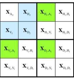
The edge map of Y is defined in a similar way for X. As an example, Fig. 2 depicts the subbands of image X for N=2. The subbands involved in computing the edge map are shown in color in this figure. It is notable that the edge map is intended to be an estimate of image edges. Thus, the most informative subbands are used in forming the edge map, rather than considering all of them. In our method, we use only 3N edge bands. If we considered all the bands in our edge map, we would have to use 4^N−1 bands.

When N is greater than or equal to 2, the value 4^N−1 is much greater than 3N. Thus, our proposed edge map helps save computation effort. According to our simulations, considering all the image subbands in calculating the edge map does not have a significant impact on increasing prediction accuracy. It is notable that the edge maps only reflect the fine-edge structures of images.

Step 4. We apply IQM between the edge maps X_E and Y_E. The resulting quality map (or score) is called the edge quality map (or score), IQM_E.

Step 5. Some metrics, like AD or SSIM, generate an intermediate quality map which should be pooled to reach the final score. In this step, we form a contrast map function for pooling the approximation and edge quality maps. It is well known that the HVS is more sensitive to areas near the edges [2]. Therefore, the pixels in the quality map near the edges should be given more importance. At the same time, high- energy (or high-variance) image regions are likely to contain more information to attract the HVS [21].

Thus, the pixels of a quality map in high-energy regions must also receive higher weights (more

importance). Based on these facts, we can combine our edge map with the computed variance to form a contrast map function. The contrast map is computed within a local Gaussian square window, which moves (pixel by pixel) over the entire edge maps X_E and Y_E. As in [8], we define a Gaussian sliding window ^W=

{

}

N E AN

2 2 0.15 E A

( , ) ( _{x x} )

Contrast x x = μ σ (9)

N N N

A A

2 K 2

A , 1

( )

k k

k

x w x x

σ μ

=

=

∑

E AN N

K K

E, A ,

1 1

,

k k k k

k k

x w x x w x

μ μ

= =

=

∑

∑

AN

x denote image patches of X_Eand

AN

X within the sliding window. It is notable that the contrast map merely exploits the original image statistics to form the weighted function for quality map pooling. Fig. 3(b) demonstrates the resized contrast map obtained by eq. (9) for a typical image in Fig.

3(a). As can be seen in Fig. 3, the contrast map nicely shows the edges and important image structures to the HVS. Brighter (higher) sample values in the contrast map indicate image structures that are more important to the HVS and play an important role in judging image quality.

(a) (b)

Fig. 3. (a) Original image; (b) Contrast map computed using eq. (9). The sample values of the contrast map are scaled between [0,255] for easy observation.

Step 6. For map-based metrics, the contrast map in (9) is used for weighted pooling of the approximation quality map IQM_A and the edge quality map IQM_E.

N N N

N

M

E, A , A A , A ,

1

M

E, A , 1

( , ) IQM ( , )

( , )

j j j j

j A

j j

j

Contrast S

Contrast

=

=

⋅

=

∑

∑

x x x y

x x

(12)

N

N

M

E, A , E E, E,

1

M

E, A , 1

( , ) IQM ( , )

( , )

j j j j

j E

j j

j

Contrast S

Contrast

=

=

⋅

=

∑

∑

x x x y

x x

(13)

where x_E,j and

A ,N j

x in the contrast map function denote image patches in the j-th local window;

A ,N j

x ,

A ,N j

y , x_E,j, and y_E,j in the quality map (or score) terms are image patches (or pixels) in the j-th local window position; M is the number of samples (pixels) in the quality map; and S_A and S_E represent the approximation and edge quality scores respectively. It is notable that, for non map-based metrics like PSNR, S_A = IQM_A and S_E = IQM_E.

Step 7. Finally, the approximation and edge quality scores are combined linearly, as defined in eq. (14), to obtain the overall quality score IQMDWT between images X and Y:

IQMDWT( , ) (1 )

0 1

A E

S S

β β

β

= ⋅ + − ⋅

< ≤

X Y (14) where IQM_DWT gives the final quality score between the images; and β is a constant. As the approximation subband contains the main image contents, β should be close to 1 to give the approximation quality score (S_A) much greater importance. We set β to 0.85 in our simulations, which means the approximation quality score constitutes 85% of the final quality score and only 15% is made up of the edge quality score.

III. EXAMPLES OF FRAMEWORK APPLICATIONS

In this section, we clarify how to apply a framework to various well-known quality assessment methods. The SSIM and VIF methods are explained in the top-down category [22],[23], and the PSNR

and AD approaches are discussed in the error-based (bottom-up) category. The SSIM and AD metrics are examples of map-based metrics, and VIF and PSNR are examples of non map-based metrics.

A. Structural SIMilarity

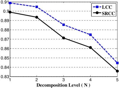
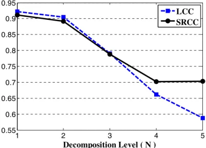
In the first step, we need to make sure that one decomposition level, as we previously proposed, works appropriately for calculating the proposed SSIM_DWT value. Since the image approximation subband plays the major role in our algorithm, we want to determine N in such a way that it maximizes the prediction accuracy of the approximation quality score SSIM_A by itself. So, using an approximation quality part with computational complexity that is lower than that of the full metric helps to predict quality accurately. The plots in Fig. 4 show the linear correlation coefficient (LCC) and Spearman’s rank correlation coefficient (SRCC) between SSIM_A and the mean opinion score (MOS) values for different N. In performing this test, all the distorted images of the IVC image database [24] were included in computing the LCC and SRCC. The distorted images in this database were generated from 10 original images using 4 different processing methods: JPEG, JPEG2000, LAR coding, and Blurring [24]. As can be seen from Fig. 4, SSIM_A achieves its best performance for N=1.

1 2 3 4 5

0.55 0.6 0.65 0.7 0.75 0.8 0.85 0.9 0.95

Decomposition Level ( N )

LCC SRCC

Fig. 4. LCC and SRCC between the MOS and mean SSIMA prediction values for various decomposition levels

In the second step, we calculate the approximation SSIM map, SSIM_A, between the approximation subbands of X and Y. For each image patch x_A and y_A within the first level approximation subbands of X and Y, SSIM_A is computed as eq. (15):

A A A A A

SSIM ( ,x y ) SSIM( ,= x y ) (15) The SSIM map is calculated according to the method in [8]. We keep all the parameters the same as those proposed in [8], except for window size, for which we use a sliding 4×4 Gaussian window.

In the third step, the edge-map function is defined for each image using eqs. (6), (7):

(

) (

) (

)

2 2 2

E( , )m n = 0.45⋅ H ( , )m n +0.45⋅ V( , )m n +0.1⋅ D( , )m n

X X X X (16)

(

) (

) (

)

2 2 2

E( , )m n = 0.45⋅ H( , )m n +0.45⋅ V( , )m n +0.1⋅ D ( , )m n

Y Y Y Y (17)

where (m,n) shows the sample position within the wavelet subbands.

In the fourth step, the edge SSIM map, SSIM_E, is calculated between two images using the following formula:

E E

E E

,

E E E 2 2

SSIM ( , ) 2 ^{x y}

x y

c c σ

σ σ

= +

+ +

x y (18) ( ) , 2 1

c= kL k (19) where

E, E

σx y is the covariance between image patches x_E and y_E (of X_E and Y_E); parameters

E

2x

σ and

E

y2

σ are variances of x_E and y_E respectively; k is a small constant; and L is a dynamic range of pixels (255 for gray-scale images). The correlation coefficient and variances are computed in the same manner as presented in [8]. In fact, as the edge map only forms image-edge structures and contains no luminance information, the luminance comparison part of the SSIM map in [8] is omitted for the edge SSIM map.

In the next steps, the contrast map is obtained using eq. (9) for pooling SSIMA and SSIME in eqs.

(12),(13). The final quality score, SSIMDWT, is calculated using eq. (14):

SSIMDWT( , )X Y = ⋅β S_A+ −(1 β)⋅S_E (20)

B. Visual Information Fidelity

The VIF index is the most accurate image quality metric, according to the performance evaluation of the prominent image quality assessment algorithms presented in [9]. In spite of its high level of accuracy, this index has not been given as much consideration as the SSIM index in a variety of applications. This is probably because of its high computational complexity (6.5 times the computation time of the SSIM, index according to [16]). Most of the complexity in the VIF index comes from over-complete steerable pyramid decomposition, in which the neighboring coefficients from the same subband are linearly correlated. Consequently, the vector Gaussian scale mixture GSM is applied for accurate quality prediction.

In this section, we explain the steps for calculating VIF in the discrete wavelet domain by exploiting the proposed framework. The proposed approach is more accurate than the original VIF index, and yet is less complex than the VIF index. It applies real Cartesian-separable wavelets and uses scalar GSM instead of vector GSM in modeling the images for VIF computation.

1) Scalar GSM-based VIF: Scalar GSM has been described and applied in the computation of the IFC [15]. We repeat that procedure here for VIF index calculation using scalar GSM. Considering Fig. 5, let

M

1 2 M

C C ,C ,…,C denote M elements from C, and let D^M D ,D ,… ,D_{1 2 M} be the corresponding M elements from D. C and D denote the RFs from the reference and distorted signals respectively (as in [15], the models correspond to one subband). C is a product of two stationary random fields (RFs) that are independent of each other:

{

} {

}

= C ∈ = ⋅ =I S U⋅ ∈I

C S U (21)

Fig. 5. Block diagram of the VIF index [16]

where I denotes the set of spatial indices for the random field (RF); S is an RF of positive scalars; and U is a Gaussian scalar RF with zero mean and variance σ_U². The distortion model is a signal attenuation and additive Gaussian noise, defined as follows:

{

} {

}

= D ∈ =I GC V+ = C V ∈I

D g (22) where G is a deterministic scalar attenuation field; and V is a stationary additive zero mean Gaussian noise RF with variance σ_V². The perceived signals in Fig. 5 are defined as follows (see [16]):

= +

E C N , F D N= + ^' (23) where N and N^'represent stationary white Gaussian noise RFs with variance σ_N². If we take the steps outlined in [16] for VIF index calculation considering scalar GSM, we obtain:

(

) (

)

1

; 1

2

i i

I I σ σ

= σ

⎛ + ⎞

= = = ⎜ ⎟

⎝ ⎠

∑

N

og

; s

C E S s C E s l (24)

In the GSM model, the reference image coefficients are assumed to have zero mean. So, for the scalar GSM model, estimates of s²_i can be obtained by localized sample variance estimation. The variance σ_U² can be assumed to be unity without loss of generality [15]. Thus, eq. (24) is simplified to eq. (25):

(

)

1

; 1 1

2

i

i

I σ

σ

=

⎛ ⎞

=

∑

N

og

C E s l ^C (25)

Similarly, we arrive at eq. (26):

(

)

1

; 1 1

2

i i

i

I σ

σ σ

=

⎛ ⎞

=

∑

V N

og g

C F s l ^C (26)

The final VIF index is defined by eq. (27), as in [16], but considering a single subband:

( )

( )

M M M

M M M

;

; VIF I

= I C F s

C E s (27)

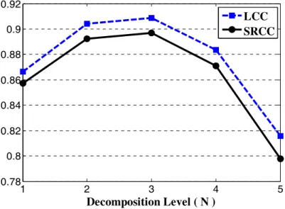
2) Description of the Computational Approach: As we explained previously in the SSIM section, we first need to verify the right number of decomposition levels to calculate the proposed VIF_DWT. We perform the experiments on an IVC image database in a similar way to that explained in the SSIM section for the scalar VIF. Fig. 6 shows the LCC and SRCC between VIF_A and the MOS values for different decomposition levels. As expected, the VIF_A prediction accuracy decreases as the number of decomposition levels increases. Therefore, VIF_A performance is best at N=1. In the second step, we calculate the approximation quality score, VIF_A, between the first-level approximation subbands of X and Y, i.e. XA and YA (for simplicity, XA and YA are used instead of

A1

X and

A1

Y here):

,

,

2 2 M

2 2 2

1 M 2

2 2

1

1

1

A i

i

A i

i i

A

i

VIF

σ σ σ

σ σ

=

=

⎛ ⎞

+

⎜ ⎟

⎜ + ⎟

⎝ ⎠

= ⎛ ⎞

+

⎜ ⎟

⎜ ⎟

⎝ ⎠

∑

∑

V N

N

og g

og l

l

x

x

(28)

where M is the number of samples in the approximation subband; x_{A i,} is the i^th image patch in the approximation subband XA; and

,

2

σ_xA i is the variance of x_{A i,} . The noise variance σ_N² is set to 5 in our approach. The parameters g_i and ²

σ_Vi are estimated as described in [16], which results in eq. (29) and eq.

(30).

, ,

,

, 2

A i A i

A i

i

σ

σ ε

= +

x y x

g (29)

where

,, , A i A i

σ_{x y} is the covariance between image patches x_{A i,} and y_{A i,} ; and ε is a very small constant to avoid instability when

,

2

σ_xA iis zero. In our approach, ε =10⁻²⁰.

, , ,

2 2

i A i i A i, A i

σ_V =σ_y − ⋅g σ_{x y} (30) All the statistics (the variance and covariance of the image patches) are computed within a local Gaussian square window, which moves (pixel by pixel) over the entire approximation subbands XA and YA. In this case, a Gaussian sliding window is used in exactly the same way as that defined in step 5 of

section II. Because of the smaller resolution of the subbands in the wavelet domain, we can even extract reasonably accurate local statistics with a small, 3×3 sliding window. But, to achieve the best performance and extract accurate local statistics, a larger, 9×9 window is used here. In the simulation section, we show that the VIF_DWT can provide accurate scores with the proposed setup.

1 2 3 4 5

0.83 0.84 0.85 0.86 0.87 0.88 0.89 0.9 0.91

Decomposition Level ( N )

LCC SRCC

Fig. 6. LCC and SRCC between the MOS and VIFA prediction values for various decomposition levels

In the third step, the edge maps XE and YE are computed using eqs. (16) and (17). Then, the edge quality score, VIFE, is calculated between edge maps, as in the second step.

Finally, the overall quality measure between images X and Y is obtained using eq. (14):

VIFDWT( , ) (1 )

0 1

A E

VIF VIF

β β

β

= ⋅ + − ⋅

< ≤

X Y (31)

where VIF_DWT gives the final quality score of images in the range [0,1].

It is worth noting that we skipped the steps for computing a contrast map (eq. (9)) and the pooling procedure as defined in the general framework. That is because the VIF is a non map-based quality score, unlike the SSIM.

C. PSNR

The conventional PSNR and the mean square error (MSE) are defined as in eqs. (32) and (33):

2

PSNR( , ) 10 10

MSE( , )

⎛ max ⎞

= ⋅ ⎜ ⎟

⎝ ⎠

X Y X

og X Y

l (32)

( )

P ,

MSE( , ) 1 ( , ) ( , )

N _{m n} m n m n

= ⋅

∑

X Y X Y (33) where X and Y denote the reference and distorted images respectively; Xmax is the maximum possible pixel value of the reference image X (the minimum pixel value is assumed to be zero); and NP is the number of pixels in each image. Although the PSNR is still popular because of its ability to easily compute quality in decibels (dB), it cannot adequately reflect the human perception of image fidelity.

Other error-based techniques, such as wSNR[6], NQM [6], and VSNR [5], are more complex to use, as they follow sophisticated procedures to compute the human visual system (HVS) parameters. In this subsection, we explain how to calculate PSNR-based quality accurately in the discrete wavelet domain using the proposed framework.

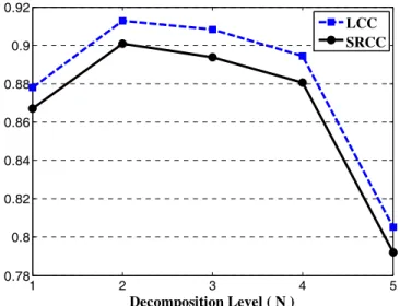
The first step is to determine the right number of decomposition levels (N) required to calculate the PSNR_DWT value. This number can be calculated using eq. (5). To make sure of the validity of eq. (5), we verify the theoretical value by comparing it with the experimental value obtained by performing tests on the IVC database. This database consists of 512×512 images that were subjectively evaluated at a viewing distance of 6 times the screen height. The plots in Fig. 7 show the LCC and SRCC between PSNR_A and the MOS values for different decomposition levels. It can be seen that PSNR_A attains its best performance at N=3. However, the prediction accuracy for N=2 is very close to that. Based on individual types of distortion, which are available in the corresponding image database, we can determine which value of N (2 or 3) provides more reliable prediction scores. Table I lists the SRCC values for four different types of distortion. It is observed that the PSNRA at N=3 performs better for all types of distortion, expect blurring. When all data (distorted images) are considered, the performance of PSNRA is superior, at N=3.

To reach a fair comparison for PSNR_DWT, we optimized that full metric with respect to constant β for each decomposition level (N=2 and N=3). When we calculated the root mean square error (RMSE) between the PSNR_DWT and MOS values for different β, which reaches its minimum (global) for β = 0.89 at N=2, and for β = 0.79 at N=3. Interestingly, these values of β are close to what is suggested in step 7 in section II, i.e. β is equal to 0.85. The value of β for N=2 is greater than its value for N=3. That is because, for larger N, the resolution of the approximation subband, and consequently the importance of its role in quality prediction, decreases. As Table I shows, the prediction accuracy of PSNR_DWT at N=3 is better than that computed at N=2 for all types of distortion. Hence, N=3 is the appropriate decomposition level for the proposed algorithm performing on the IVC database.

The SRCC value for the PSNR_DWT at N=3 is 0.9511, which is higher than the value of 0.9368 at N=2.

This shows the effectiveness of the proposed edge-map function in improving prediction accuracy, especially for the low-pass filtering type of distortion.

Now, we use eq. (5) to compute the appropriate number of decomposition levels for the IVC database.

For that database, k is equal to 6. Thus,

( )

( )

(

)

N_IVC =max 0,round log 512 / 57.33 =3 (34) It can be observed that the theoretical value of N obtained in eq. (34) exactly matches the experimental value explained previously.

We must point out that the LCC has low sensitivity to small variations in β, that is, the proposed β = 0.85 does not drastically affect PSNRDWT performance compared with the optimum β value for the quality prediction across different image databases.

In the second step, the edge-map functions of images X and Y are computed by eq. (6). Then, we calculate the approximation quality score PSNRA and the edge quality score PSNRE using eq. (32), as defined in eq. (35) and eq. (36):

N N

A A A

PSNR =PSNR(X ,Y ) (35)

E E E

PSNR =PSNR(X Y, ) (36)

Finally, the overall quality score PSNR_DWT is computed by combining approximation and edge quality scores according to eq. (14):

DWT A E

PSNR ( , )X Y = ⋅β PSNR + −(1 β) PSNR , 0⋅ < ≤β 1 (37) where PSNRDWT gives the final quality score of the images in dB.

1 2 3 4 5

0.78 0.8 0.82 0.84 0.86 0.88 0.9 0.92

Decomposition Level ( N )

LCC SRCC

Fig. 7. LCC and SRCC between the MOS and PSNRA prediction values for various decomposition levels

TABLE I

SRCC VALUES FOR DIFFERENT TYPES OF IMAGE DISTORTION IN THE IVCIMAGE DATABASE Distortion PSNR_A (N=2) PSNR_A (N=3) PSNRDWT

(N=2)

PSNRDWT

(N=3)

JPEG 0.8482 0.8699 0.8505 0.865

JPEG2000 0.9210 0.934 0.9262 0.9315

Blur 0.9308 0.9112 0.9368 0.9511

LAR 0.8262 0.8798 0.8668 0.8861

All Data 0.8924 0.8971 0.8964 0.906

D. Absolute Difference (AD)

To verify the performance of our framework more generally, we investigate how it works if the AD of the images is considered as the IQM. As in previous cases, we first need to know the required number of decomposition levels in order to calculate the AD_DWT value. When we perform a test on the IVC image

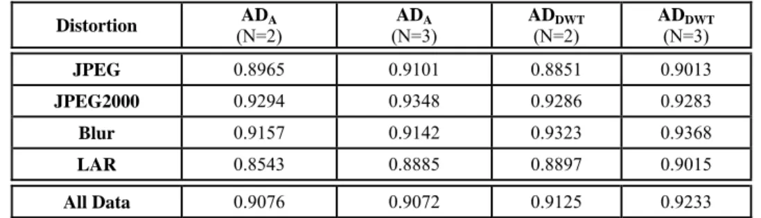
database in the same way as before, Fig. 8 is obtained, which shows the LCC and SRCC between the mean AD_A and MOS values for different decomposition levels. Like the PSNR_A, the AD_A performs well at N=2 and N=3. Table II shows SRCC values between the AD-based metrics and MOS values for two and three decomposition levels. According to Table II, the performances of the AD_A and AD_DWT at N=3 are better than N=2 for individual types of distortion. Like the computation of PSNR_DWT in the previous subsection, we optimized AD_DWT with respect to constant β, which results in β = 0.89 for N = 2 and β = 0.72 for N = 3. When the value of N is calculated by eq. (5), the result is three levels of decomposition for the IVC database that match the experimental value.

In the second step, we calculate the approximation AD map, AD_A, between the approximation subbands of X and Y.

N N

A A A

AD ( , )m n = X ( , )m n −Y ( , )m n (38) where (m,n) shows a sample position in the approximation subband.

In the third step, the edge-map function images X and Y are defined in eqs. (6),(7), and the edge AD map, AD_E, is calculated between the edge maps X_E and Y_E in the next step.

E E E

AD ( , )m n = X ( , )m n −Y ( , )m n (39) In the fourth step, the contrast map is obtained using eq. (9), and then ADA and ADE are pooled using the contrast map to calculate the approximation and edge quality scores SA and SE.

M

A 1

M

1

( , ) AD ( , ) ( , )

j A

j

Contrast m n m n S

Contrast m n

=

=

⋅

=

∑

∑

(40)

M

E 1

M

1

( , ) AD ( , ) ( , )

j E

j

Contrast m n m n S

Contrast m n

=

=

⋅

=

∑

∑

(41)

The final quality score, ADDWT, is calculated using eq. (42).

ADDWT( , )X Y = ⋅β S_A+ −(1 β)⋅S_E (42)

1 2 3 4 5

0.78 0.8 0.82 0.84 0.86 0.88 0.9 0.92

Decomposition Level ( N )

LCC SRCC

Fig. 8. LCC and SRCC between the MOS and mean ADA prediction values for various decomposition levels

TABLE II

SRCC VALUES FOR DIFFERENT TYPES OF IMAGE DISTORTION IN THE IVCIMAGE DATABASE Distortion ADA

(N=2) ADA

(N=3) ADDWT

(N=2) ADDWT

(N=3)

JPEG 0.8965 0.9101 0.8851 0.9013

JPEG2000 0.9294 0.9348 0.9286 0.9283

Blur 0.9157 0.9142 0.9323 0.9368

LAR 0.8543 0.8885 0.8897 0.9015

All Data 0.9076 0.9072 0.9125 0.9233

E. Computational Complexity of the Algorithms

In spite of the number of steps required to calculate the final quality score, the computational complexity of the proposed algorithms is low. Here, we discuss various different aspects of the complexity of the approach. The resolution of the approximation subband and edge map is a quarter of that of the original image. Lower resolutions mean that fewer computations are required to obtain the image statistics or quality maps, e.g. SSIM maps for the SSIM_DWT. Because of the smaller resolution of the subbands in the wavelet domain, we can extract accurate local statistics with a smaller sliding window. For example, the spatial SSIM in [8] uses an 11×11 window by default, while in the next section we show that the SSIMDWT can provide accurate scores with a 4×4 window. A smaller window reduces

the number of computations required to obtain local statistics. As can be seen from eq. (9), the local statistics calculated for eq. (15) and eq. (18) are used to form the contrast map. Therefore, in computing SSIM_DWT, the contrast map does not impose a large computational burden.

Probably the most complex part of the approach is wavelet decomposition. A simple wavelet can be used to reduce complexity. We used the Haar wavelet for image decomposition. As this wavelet has the shortest filter length, it makes the filtering process simpler. The use of the Haar wavelet makes it possible to calculate VIF_DWT using the scalar GSM model with a complexity of about 5% of the original VIF index, which uses an over-complete steerable pyramid transform. Furthermore, the use of the Haar wavelet enables us to investigate the computational complexity of simple algorithms, e.g. PSNR_DWT, mathematically and compare them to other methods like PSNR, as explained below.

To calculate the PSNR between two images, we need 1 subtraction, 1 multiplication (square), and 1 addition for every input pixel. Therefore, this calculation requires 3 operations per input pixel.

In the decomposition stage, one operation per input pixel must be performed to obtain a desired image subband using the Haar wavelet. That is because the Haar wavelet is actually a simple averaging. For example, to obtain the second level approximation subband, we need to perform 15 additions and 1 shift (as a division) for every 4×4=16 neighboring pixels, which results in 1 operation per input pixel. As we apply the DWT to both the reference and the distorted images, we need (2+3/(4^N)) operations per input pixel to calculate PSNRA (with N-level wavelet decomposition). Since N is greater than or equal to unity (N ≥ 1), the computational complexity of PSNR_A is less than that of the PSNR. However, in the next section, we show that PSNR_A is much more accurate than the PSNR in predicting quality scores.

In order to calculate PSNR_E, we first need to compute edge maps for the reference and distorted images. By analyzing eq. (6), eq. (7), and eq. (36), we find that the number of operations per input pixel for calculating PSNR_E is found as in eq. (43) (considering the square root as s operations):

( )

E

N N

N

# (PSNR )

3 1

2N 3 (8 s) / 4 3 2N 1 N(16 2s) 4 (43)

4 3 /

of operations per input pixel =

⋅ + + + = ⋅⎛ +⎛ + + ⎞ ⎞

⎜ ⎟

⎜ ⎝ ⎠ ⎟

⎝ ⎠

The value of s is about 30 for Intel processor architectures [25]. For instance, for an N of 2, the complexity of PSNR_E is about 7.2 times that of the PSNR (and about 7 times greater for N=3). A comparison based on a C++ implementation of SSIM shows that, for a 640×480 image, it is approximately 115 times more complex than the PSNR. Thus, calculation of PSNR_DWT is not computationally expensive relative to other metrics. However, we should mention that PSNR_A alone gives very accurate scores, while PSNR_E is most effective when taking into account certain distortions, like fast fading channel distortion.

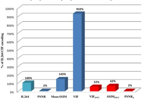
In order to develop a practical concept of the complexity of the various metrics, we chose the complexity of IPP-based H.264 baseline encoding [26] for CIF-sized videos as the benchmark and compared it to the complexity of some of the metrics. In order to verify the computational complexity of those metrics, we measured the execution time of the algorithm based on the elapsed CPU time. Fig. 9 shows the bar graph of quality metric complexity versus H.264 CIF encoding. We used C/C++

implementations for timing measurement. As can be observed from Fig. 9, the computational complexity of PSNR and PSNRA is about 2% of the H.264 encoding. In the next section, we show that PSNRA

prediction accuracy is much greater than that of conventional PSNR.

0%

100%

200%

300%

400%

500%

600%

700%

800%

900%

1000%

H.264 PSNR Mean SSIM VIF 100%

2%

143%

932%

52% 62%

2%

% of H.264 CIF encoding

Quality metric complexity vs. H.264 CIF encoding

VIF_DWT SSIM_DWT PSNR_A

Fig. 9. Comparison of the complexity of various quality metrics vs. H.264 encoding complexity

IV. SIMULATION RESULTS

In the previous section, we used the IVC image database for some verification with respect to decomposition levels. In this section, the performance of the proposed algorithm for the quality calculation is evaluated on the LIVE Image Quality Assessment Database, Release 2 [27]. This database consists of 779 distorted images derived from 29 original color images using five types of distortion:

JPEG compression, JPEG2000 compression, Gaussian white noise (GWN), Gaussian blurring (GBlur), and the Rayleigh fast fading (FF) channel model. The realigned subjective quality data for the database are used in all experiments [27].

In this paper, two performance metrics are applied, in addition to the statistical F-test, to measure the performance of the objective models. The first metric is the Pearson correlation coefficient (LCC) between the Difference Mean Opinion Score (DMOS) and the objective model outputs after nonlinear regression. The correlation coefficient gives an evaluation of prediction accuracy. We use the five- parameter logistical function defined in [9] for nonlinear regression. The second metric is the Spearman rank correlation coefficient (SRCC), which provides a measure of prediction monotonicity.

In order to put the performance evaluation of our proposed scheme into the proper context, we compare our quality assessment algorithms with other quality metrics, including the conventional PSNR, the spatial domain mean SSIM [8], an autoscale version of SSIM that performs downsampling on images [28], and a weighted SNR (wSNR) [6], in which the images are filtered by the CSF specified in [29] and [30]. For the LIVE database, we set k at eq.(5) equal to 3, based on the experimental setup and the decomposition level calculated for each image using eq. (5).

Tables III and IV show the results of performance metrics for each type of image distortion in the LIVE database. To understand the effect of the contrast map (eq. (9)) in improving quality prediction, we can compare the results of the mean SSIM_A and S_A rows in the corresponding tables. It is observed that the SRCC of the mean SSIM_A increases from 0.9441 to 0.9573 for S_A, which corresponds to a 1.32%

improvement. The performance of SSIM_DWT is the best of all the structural metrics. For SNR-based

metrics, the SRCC of PSNR_A is 0.9307, which is higher than that of conventional PSNR (0.8756) and even wSNR (0.9240), while its complexity is lower than that of conventional PSNR. The performance of PSNR_DWT is better than PSNR_A for GWN, GBlur, and FF types of distortion. To verify the validity of the proposed framework, we check the performance of AD_DWT. Table IV shows that its performance is close to mean SSIM_A and SSIM_autoscale. The SRCC value for VIF_DWT is 0.9681, which is higher than the SRCC value of the VIF index (0.9635) defined in [16]. VIF_DWT has the best performance of all the image quality metrics we describe here.

To assess the statistical significance of each metric’s performance relative to that of other metrics, a two-tailed F-test was performed on the residual differences between the IQM predictions and the DMOS.

The F-test is used to determine whether one metric has significantly larger residuals (greater prediction error) than another [31]. The F-statistic is defined by a ratio of variances of prediction errors (residuals) from two image quality metrics. The more this ratio deviates from 1, the stronger the evidence for unequal population variances. Values of F > F_critical or F < 1/F_critical indicate that residuals resulting from one quality metric are statistically distinguishable from the residuals of another quality metric (i.e.

significantly larger or smaller). Fcritical is computed based on the number of residuals and a significance level of α. In this paper, we used α = 0.05, which results in Fcritical = 1.151. Table V shows the F-statistic obtained based on the residuals from each structurally based metric against the residuals from SSIMautoscale. It is observed that SSIMDWT has significantly smaller residuals than SSIMautoscale, and SSIMspatial has significantly larger residuals than SSIMautoscale. Results in Table VI show that the proposed VIFDWT outperforms the VIF index when all the distorted images are considered. F-statistic values for error-based metrics are presented in Table VII. As can be seen, the performance of ADDWT is statistically superior to that of the other error-based models.

Fig. 10 shows the scatter plots of DMOS vs. various quality metrics for all the distorted images. It is evident that the SSIM_DWT, PSNR_DWT, and VIF_DWT predictions are more linear and more uniformly scattered compared to other models.