ON THE STABILITY OF THE MOTION FOR A NEO-HOOKEAN SYSTEM

(1)

1

ON THE STABILITY OF THE MOTION FOR A NEO-HOOKEAN

SYSTEM

Nicolae–Doru Stănescu

University of Piteşti, Department of Applied Mechanics, Piteşti, Romania

Abstract

It is well known that the vibrations are a major cause for the instability in the mechanical systems and major source of noises. In this paper we propose a simple system with two degrees of freedom based on a non-linear elastic element. For this system, it is proved in the present paper that the motion is stable, but not asymptotically stable. A comparison between the non-linear case and the linear case is performed, and for the both cases the eigenpulsations are also determined. All theoretical results are validated by numerical simulation.

Keywords: neo-Hookean, motion, stability, numerical validation.

1. Introduction

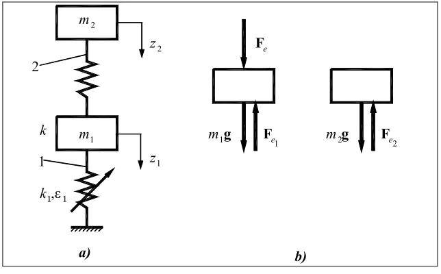
The system purposed for the study is described in figure 1, a. It consists of the masses m₁ and m₂

linked one to another by the linear spring of stiffness k . The mass m₁ can be considered to be the foundation of the machine-tool, and the mass m₂ the machine-tool itself. The mass m₂ is linked to the ground by the non-linear spring 1 for which the elastic force writes

2 1 1

x x k

F= − ε , (1)

where x is the elongation of the spring. The fundamental working hypothesis is that

0

1>

ε . (2)

The system has two degrees of freedom, that is the displacements z₁ and z₂ of the two masses in the vertical direction.

2. The equations of motion

(2)

2

b) a)

2

e

F

m2g g

1

m

1 F_e

e

F

1 2

2

z

1

z k

2

m

1

m

ε₁

, 1

[image:2.595.137.459.98.298.2]

k

Figure 1 – The mathematical model

(

z z

)

mg

k z z k z

m ₂ ₂ ₁ ₁

1 1 1 1 1

1 + − +

ε + − =

&

& _,

(

)

1 2 2

2

2z m g k z z

m && = − − _, ₍₃₎

where g is the gravitational acceleration. Denoting

1

1=z

ξ , ξ₂ =z₂, ξ₃ =z&₁_,

2 4 =z&

ξ , (4)

the relations (3) transform in a system of four first order non-linear differential equations,

3

1 =ξ

ξ&

, ξ&₂ =ξ₄,

(

)

_

  

 

+ ξ − ξ + ξ ε + ξ − =

ξ k k mg

m ₁2 2 1 1

1 1 1 1 3

1

&

,

[

₂

(

₂ ₁

)

]

2 4

1

ξ − ξ − =

ξ m g k

m &

. (5)

3. The equilibrium positions

These positions found at the intersections of the nullclines, so that one obtains the system

0

3 =

ξ , ξ₄ =0,

(

₂ ₁

)

₁ 0

2 1 1 1

1 _ξ + ξ −ξ + =

ε + ξ

−k k mg , m₂g−k

(

ξ₂−ξ₁

)

=0. ₍₆₎

Summing the last two relations (6), it results

(

₁ ₂

)

0

2 1 1 1

1 _ξ + + =

ε + ξ

−k m m g , ₍₇₎

wherefrom

(

₁ ₂

)

₁2 ₁ 0 3

1

1ξ − m +m gξ −ε =

k . (8)

(3)

3

(

₁ ₂

)

₁2 ₁ 0 3

1

1ξ + m +m gξ +ε =

k (9)

for which there exists no variation of sigh in the sequence of the coefficients so that the Descartes theorem assures us that we have no negative real root for the equation (8). In conclusion, the equation (8) has exactly one positive real root, name it ξ₁.

The last relation (6) becomes now a linear equation in the unknown ξ₂ and therefore it has only one solution,

1 2

2 = +ξ

ξ

k g m

. (10)

We proved in this way that the system has only one equilibrium position

(

ξ₁,ξ₂,0,0

)

. Let us denote by f

( )

ξ₁ the function f :_R→_R,

( )

(

)

2 ₁

1 2 1 3 1 1

1 = ξ − + ξ −ε

ξ k m m g

f (11)

for which the derivative is

( )

(

1 2

)

1

2 1 1

1 =3 ξ −2 + ξ

ξ

′ k m m g

f . (12)

The equation f′

( )

ξ₁ =0 has the solutions

( )1 ₀

1 =

ξ , ( )

(

)

1 2 1 2

1

3 2

k g m

m +

=

ξ , (13)

( )1 1

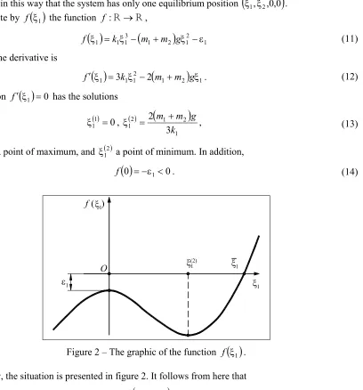
ξ being a point of maximum, and ξ₁( )2 a point of minimum. In addition,

( )

0 =−ε₁<0

f . (14)

ε₁

O

ξ₁ ξ₁

1

ξ

(2)

f ( )

[image:3.595.122.530.246.684.2]

ξ₁

Figure 2 – The graphic of the function f

( )

ξ₁ .

Graphically, the situation is presented in figure 2. It follows from here that

(

)

1 2 1 1

3 2

k g m

m +

>

(4)

4

4. The stability of the equilibrium

Let us denote by f_k, k =1,4 the right-hand terms of the relations (5) and by j_kl the partial derivatives

l k kl

f j

ξ ∂ ∂

= , k =1,4, l=1 ,4. ₍₁₆₎

We have

0

11=

j , j₁₂=0, j₁₃=1, j₁₄ =0, (17)

0

21=

j , j₂₂=0, j₂₃=0, j₂₄ =1, (18)

    

  

ξ ε − − −

= ₃

1 1 1

1 31

2 1

k k m

j ,

1 32

m k

j = , j₃₃=0, j₃₄ =0, (19)

2 41

m k

j = ,

2 42

m k

j =− , j₄₃ =0, j₄₄=0. ₍₂₀₎

The characteristic equation

(

)

0

det J−λI = (21)

in which J is the Jacobi matrix,

[ ]

4 , 1

= =

=

l k kl

j

J , and I is the fourth order unity matrix, reads

0

0 0 1 0 0

0 1 0

42 41

32 31

=

λ − λ − λ − λ −

j j

j

j . (22)

Multiplying the third column by λ and adding it to the first column, the fourth column by λ and adding it to the second column, results the equation

(

₃₁ ₄₂

)

2 ₃₁ ₄₂ ₃₂ ₄₁ 0

4 ₋ ₊ _λ ₊ ₋ ₌

λ j j j j j j . (23)

From the Routh–Hurwitz criterion we deduce that the equation has not all the roots with negative real part and therefore the equilibrium can not be asymptotically stable.

On the other hand, the roots of the equation (23) are

(

)

2

4 ₃₂ ₄₁ 2

42 31 42

31 2 1

j j j

j j

j + ± − +

=

λ . (24)

Keeping into account the expressions (17)-(20), we have

0 2

2 1

3 1 1 1

42

31 − <

ξ ε + + − = +

m k m

k k

j

j , (25)

0 4 4

2 1

2

41

32 = >

m m

k j

(5)

5

(

j₃₁− j₄₂

)

2 +4j₃₂j₄₁>0, (27) More,

(

)

2 ₃₂ ₄₁

42 31 42

31 j j j 4j j

j + > − + (28)

because it is equivalent to

41 32 42

31j j j

j > , (29)

that is

2 1

2

2 3 1 1

2 1

2

2 1

1 2

m m

k m

m k m m

k k

> ξ

ε +

+ . (30)

The previous relations assure us that λ2₁<0, λ2₂ <0 so that the roots of the characteristic equation (23) are all pure imaginary. The equilibrium position

(

ξ₁,ξ₂,0,0

)

is simply stable.

5. The stability of the motion

Let

(

ξ₁,ξ₂,ξ₃,ξ₄

)

a solution of the system (5) and

(

u₁,u₂,u₃,u₄

)

a deviation sufficiently small in its norm. We can write

3 3 1

1+u =ξ +u

ξ& & _,

4 4 2

2+u =ξ +u

ξ& & _,

(

)

(

)

(

)

_

 

  

+ − + ξ − ξ + + ξ

ε + + ξ − = +

ξ k u u m g

u u

k m

u ₂ ₁ ₂ ₁ ₁

2 1 1

1 1

1 1 1 3 3

1

&

& _,

(

)

[

2 2 1 2 1

]

2 4 4

1

u u k

g m m

u = − ξ −ξ + −

+

ξ& & _.

(31)

Since u₁ <<ξ₁ we can approximate

(

)

3 1

1 1 2 1 1 2 1 1

1 2 _u

u ξ

ε − ξ

ε ≈ + ξ

ε

. ₍₃₂₎

Keeping into account that

(

ξ₁,ξ₂,ξ₃,ξ₄

)

is a solution of the system (5), from the relations (31) and (32) we obtain the system in deviations

3

1 u

u& = _,

4

2 u

u& = _,

(

)

_

  

 

− + ξ ε − −

= ₃ ₂ ₁

1 1 1 1 1 1 3

2 1

u u k u u

k m

u& _,

[

(

)

]

1 2 2 4

1

u u k m

u& = − − _, ₍₃₃₎

wherefrom

(

₂ ₁

)

3 1 1 1 1 1 1 1

2

u u k u u

k u

m + −

ξ ε − − =

&

& _,

1 2 2

2u ku ku

m && =− + _. ₍₃₄₎

(6)

6 2 2 2 1 u k u m

u = && + ,

( ) 2 2 2 1 u k u m u iv & & &

& = + _, ₍₃₅₎

the first relation (34) offering now

( ) 2 ₀

2 2 1 3 1 1 1 2 2 2

1 ₊ ₌

        +         ξ ε + +

+ k k m u ku

k m u

k m

m iv _&_&

. (36)

The characteristic equation reads now

0 2 2 1 3 1 1 1 2 4 2

1 ₊ ₌

        +         ξ ε + +

+ k k m r k

k m r k m m

. (37)

The discriminate of this equation is

(

)

(

)

2

(

)

2 0

4 2 3 1 1 1 2 1 2 2 1 2 2 1 2 2 1 2 1 3 1 1 1 2 >         ξ ε + + +     ₊ + − = −         +       ξ ε + + = ∆ k k m m m k k k m m m m m m k k k m (38)

and, in addition,

2 1 3 1 1 1 2 2         +         ξ ε + + <

∆ k k m

k m

. (39)

Keeping into account that

0 2 1 3 1 1 1

2 ₊ _>

        ξ ε + +

= k k m

k m

a (40)

it immediately results that r₁2 <0, r₂2 <0 so that the roots of the characteristic equation (37) are all pure imaginary, the motion being stable, but not asymptotically stable.

The solution of the equation (36) is

            ϕ + ∆ + +             ϕ + ∆ − = ₂ 2 1 2 1 2 1 1

2 cos ₂ cos ₂ t

m m k a C t m m k a C

u . (41)

By twice derivation of the expression (41), we obtain

            ϕ + ∆ + ∆ + −             ϕ + ∆ − ∆ − − = ₂ 2 1 2 2 1 1 2 1 1 2 1

2 ₂ cos ₂ ₂ cos ₂ t

m m k a C m m k a t m m k a C m m k a

u&& ₍₄₂₎

(7)

7             ϕ + ∆ +             + ∆ + − +             ϕ + ∆ −             + ∆ − − = ₂ 2 1 2 2 1 2 1 2 1 1 2 1 2

1 ₂ 1 cos ₂ ₂ 1 cos ₂ t

m m k a C m m k a k m t m m k a C m m k a k m

u . (43)

Everywhere C₁, C₂, ϕ₁ and ϕ₂ are constants of integration, which result from the initial conditions

( )

10

1 0 u

u = , u₂

( )

0 =u₂₀, u&₁

( )

0 =u&₁₀_,

( )

20

2 0 u

u& = & _.

The expressions (41) and (43) approximate the solution of the system in deviations (31).

6. The small oscillations around the equilibrium position

These can be obtained as a particular case of the previous paragraph for

1

1 =ξ

ξ . (44)

Result the eigenpulsations

2 1 2 1 2 1 3 1 1 1 2 1 3 1 1 1 2 1 ₂ 4 2 2 m m k m m m k k k m m k k k m −         +         ξ ε + + − +         ξ ε + + = ω , 2 1 2 1 2 1 3 1 1 1 2 1 3 1 1 1 2 2 ₂ 4 2 2 m m k m m m k k k m m k k k m ₋         +       ξ ε + + + +       ξ ε + + = ω (45)

7. Comparison with the linear case

The linear case is obtained for ε₁=0. The equation (7) writes

(

₁ ₂

)

0

1

1ξ + + =

−k m m g , (46)

with the solution

( ) _g

k m m l 1 2 1 1 + =

ξ . ₍₄₇₎

One observes that ξ₁( )l <ξ₁ for which holds true the relation (15). The relation (10) offers

( ) _g

(8)

8 and therefore ξ₂( )l <ξ₂, too.

The equilibrium remains again simply stable because the relations (25)-(30) still hold true. The motion is again simply stable and we have in addition

( )

(

)

2

(

)

,

4

1 2 1 2 2 1 2 2 1 2

2 1 2 1 2 1 2

k k m m m k

k m m

m

m m k

k m m m

l

+ +       + − =

−    



 ₊ ₊

= ∆

(49)

( )

k k m m m

al = ₂ + ₁+ 2 1, ₍₅₀₎

with

( ) _>₀

∆l _, _∆( )l _<_∆_,_a( )l _>₀_,_a( )l _<_a_. ₍₅₁₎

The eigenpulsations are

( )

2 1

2 1 2 1 2 1 2 1

2 1 2

1 ₂

4

m m

k

m m k

k m m m k

k m m m

l

−    



 ₊ ₊

− + + =

ω ,

( )

2 1

2 1 2 1 2 1 2 1

2 1 2

2 ₂

4

m m

k

m m k

k m m m k

k m m m

l

−    



 ₊ ₊

+ +

+ =

ω .

(52)

8. Numerical application

Let us consider the case

kg 2000

1 =

m , m₂ =1000kg, g=10m/s2, k₁=106 N/m, ε₁=700Nm2, k =105 N/m. (53)

The equation (8) leads us to

0 700 10

3000

106ξ₁3− × ξ₁2− = (54)

with the solution

m 1 . 0

1=

ξ . (55)

The relation (10) offers us

m 2 . 0 1 . 0 10

10 1000

5

2 + =

× =

ξ . (56)

(9)

9

(

)

m 02 . 0 10 3 10 1000 2000 2 m 1 . 0 6 = × × + ×

> . (57)

The equations (17)-(20) lead us to

1250 1 . 0 700 2 10 10 2000 1 3 5 6

31 =−

     × − − − × =

j , 50

2000 105

32 = =

j , 100

1000 105

41 = =

j ,

50 2000

105

42 =− =−

j ,

(58)

the roots of the characteristic equation (23) being (24)

(

)

2 100 50 4 50 1250 50 1250 2 2 1 × × + + − ± − − =

λ , λ2₁ =−45.848, λ2₂ =−1254.152. (59)

The parameters a and ∆ are

27000 2000 1 . 0 700 2 10 10 10 1000 3 5 6

5 _+ =

 



 ₊ ₊ ×

=

a , (60)

721000000 1000 2000 4 2000 1 . 0 700 2 10 10 10 1000 2 3 5 6

5  − × × =

     +       ₊ ₊ × =

∆ . ₍₆₁₎

The eigenpulsations read

1 -5

1 38.543s

1000 2000 10 2 721000000 27000 = × × − =

ω , ₁ ₅ 733.835s-1

1000 2000 10 2 721000000 27000 = × × + = ω (62)

In the linear case we have

( ) ₁₀ ₀_.₀₃_m

10 1000 2000

6

1 × =

+ =

ξl

, ( ) 10 0.13m

10 1000 2000 10 10 1000 6 5

2 × =

+ + × =

ξl

, (63)

( ) ₁₃₀₀₀

10 10 1000 2000 1000 ₅ 6 = × + + = l

a , (64)

( ) ₄ ₂₀₀₀ ₁₀₀₀ _161000000

10 10 1000 2000 1000 2 5 6 = × × −       × + + =

∆l _, ₍₆₅₎

( ) 1

5

1 55.805s

1000 2000 10 2 161000000 13000 -l ₌ × × − =

ω , ( )₂ ₅ 506.839s1

1000 2000 10 2 161000000 13000 -l ₌ × × + = ω . (66)

One observes that

( )l

1

1 <ω

ω , ω₂ >ω( )₂l , (67)

(10)

10

0.08 0.1 0.12

0 0.5 1 1.5 2 2.5 3

t [s]

x

i_

1

[

m

]

0.19 0.2 0.21 0.22

0 0.5 1 1.5 2 2.5 3

t [s]

x

i_

2

[

m

]

-0.4 -0.2 0 0.2 0.4

0 0.5 1 1.5 2 2.5 3

t [s]

x

i_

3

[

m

/s

]

-0.15 -0.1 -0.05 0 0.05 0.1 0.15

0 0.5 1 1.5 2 2.5 3

t [s]

x

i_

4

[

m

/s

[image:10.595.124.473.99.357.2]

]

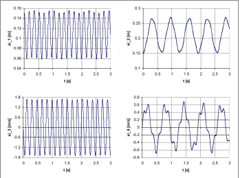
Figure 3 – The time history for the system with parameters (53) and the initial conditions (68).

0.04 0.06 0.08 0.1 0.12 0.14 0.16

0 0.5 1 1.5 2 2.5 3

t [s]

x

i_

1

[

m

]

0.1 0.15 0.2 0.25 0.3

0 0.5 1 1.5 2 2.5 3

t [s]

x

i_

2

[

m

]

-1.8 -1.2 -0.6 0 0.6 1.2 1.8

0 0.5 1 1.5 2 2.5 3

t [s]

x

i_

3

[

m

/s

]

-0.8 -0.6 -0.4 -0.2 0 0.2 0.4 0.6 0.8

0 0.5 1 1.5 2 2.5 3

t [s]

x

i_

4

[

m

/s

]

In figure 3 are represented the diagrams ξ_i

( )

t , i=1 ,4 for the parameters (53) the initial conditions being

m 11 . 0

10 =

[image:10.595.124.473.390.649.2]

(11)

11

0.04 0.06 0.08 0.1 0.12 0.14 0.16

0 0.5 1 1.5 2 2.5 3

t [s]

x

i_

1

[

m

]

0.1 0.15 0.2 0.25 0.3

0 0.5 1 1.5 2 2.5 3

t [s]

x

i_

2

[

m

]

-1.8 -1.2 -0.6 0 0.6 1.2 1.8

0 0.5 1 1.5 2 2.5 3

t [s]

x

i_

3

[

m

/s

]

-0.8 -0.6 -0.4 -0.2 0 0.2 0.4 0.6 0.8

0 0.5 1 1.5 2 2.5 3

t [s]

x

i_

4

[

m

/s

[image:11.595.124.472.113.371.2]

]

-0.005 -0.0025 0 0.0025 0.005

0 0.5 1 1.5 2 2.5 3

t [s]

x

i_

1

[

m

]

-0.005 -0.0025 0 0.0025 0.005

0 0.5 1 1.5 2 2.5 3

t [s]

x

i_

2

[

m

]

-0.2 -0.15 -0.1 -0.05 0 0.05 0.1 0.15 0.2

0 0.5 1 1.5 2 2.5 3

t [s]

x

i_

3

[

m

/s

]

-0.04 -0.03 -0.02 -0.01 0 0.01 0.02 0.03 0.04

0 0.5 1 1.5 2 2.5 3

t [s]

x

i_

4

[

m

/s

]

Figure 6 – The deviated motion between the systems captured in figures 4 and 5.

In figure 4 are represented the same diagrams for

m 15 . 0

10 =

[image:11.595.123.473.403.662.2]

(12)

12 in figure 5 for

m 151 . 0

10 =

ξ , ξ₂₀ =0.149m, ξ₃₀ =0.1m/s, ξ₄₀ =0.02m/s, (70)

and in the figure 6 the deviated motion between the two cases from figures 5 and 6.

9. Conclusions

In this paper we presented a study concerning the influence of the non-linear neo-Hookean elements on the stability of the system machine-tool-foundation. We proved that both the equilibrium and the motion are simply stable and the neo-Hookean element increases the safety domain where the resonance doesn’t appear.

References

[1] Stănescu, N.–D., Munteanu, L., Chiroiu, V., Pandrea, N., Dynamical systems. Theory and

applications, vol. 1, The Publishing House of the Romanian Academy, Bucharest (Romania),

2007.

[2] Stănescu, N.–D., Munteanu, L., Chiroiu, V., Pandrea, N., Dynamical systems. Theory and

applications, vol. 2, The Publishing House of the Romanian Academy, Bucharest (Romania), 2009

(in press).

[3] Pandrea, N., Stănescu, N.–D., Mechanics, Didactical and Pedagogical Publishing House, Bucharest (Romania), 2002.

[4] Stănescu, N.–D., Numerical methods, Didactical and Pedagogical Publishing House, Bucharest (Romania), 2007.

[5] Teodorescu, P.P., Stănescu, N.–D., Pandrea, N., Numerical analysis with applications to