BIBLIOTECAS DEL TECNOLÓGICO DE MONTERREY
PUBLICACIÓN DE TRABAJOS DE GRADO
Las Bibliotecas del Sistema Tecnológico de Monterrey son depositarias de los trabajos recepcionales y de grado que generan sus egresados. De esta manera, con el objeto de preservarlos y salvaguardarlos como parte del acervo bibliográfico del Tecnológico de Monterrey se ha generado una copia de las tesis en versión electrónica del tradicional formato impreso, con base en la Ley Federal del Derecho de Autor (LFDA).
Es importante señalar que las tesis no se divulgan ni están a disposición pública con fines de comercialización o lucro y que su control y organización únicamente se realiza en los Campus de origen.
Cabe mencionar, que la Colección de Documentos Tec, donde se encuentran las tesis, tesinas y
disertaciones doctorales, únicamente pueden ser consultables en pantalla por la comunidad del Tecnológico de Monterrey a través de Biblioteca Digital, cuyo acceso requiere cuenta y clave de acceso, para asegurar el uso restringido de dicha comunidad.
El Tecnológico de Monterrey informa a través de este medio a todos los egresados que tengan alguna inconformidad o comentario por la publicación de su trabajo de grado en la sección Colección de
Documentos Tec del Tecnológico de Monterrey deberán notificarlo por escrito a http://biblioteca.itesm.mx
Performance of Wireless Networks Using Migration Processes
for Mobility Modeling -Edición Única
Title Performance of Wireless Networks Using Migration
Processes for Mobility Modeling -Edición Única
Authors Eric Baca Sánchez
Affiliation Campus Monterrey
Issue Date 2002-05-01
Item type Tesis
Rights Open Access
Downloaded 19-Jan-2017 09:05:22
Instituto Tecnologico y de Estudios Superiores de
Monterrey
Campus Monterrey
Division de Graduados en Electronica, Computacion, Informacion
y Comunicaciones
Programa de Graduados
Performance of Wireless Networks using Migration Processes
for Mobility Modeling
THESIS
Presented as a partial fulfillment of the requirements for the degree of
Master in Sciences in Electronic Engineering
Major in Telecommunications
Ing. Eric Baca Sanchez
Instituto Tecnologico y de Estudios Superiores de
Monterrey
Campus Monterrey
Division de Electronica, Computacion, Informacion, y
Comunicaciones
Programa de Graduados
The members of the thesis committee recommended the acceptance of the thesis of Eric Baca Sanchez as a partial fulfillment of the requirements for the degree of
Master in Science in:
Electronic Engineering
Major in Telecommunications
THESIS COMMITTEE
Ph.D. Cesar Vargas Rosales Advisor
PljD. Jerge Agustin Olvera Rodriguez Synodal
Approved
lazar Director oTThe gfaduate Program
Mayo 2002
Acknowledgements
I want to thank Organization of American States (OAS-OEA) for the opportunity to perform graduate studies at the Instituto Tecnologico y de Estudios Superiores de Monterrey.
I am grateful to my thesis advisor, Cesar Vargas Rosales, Ph.D., because this thesis could not have been possible without his interest and collaboration.
I also want to thank Jorge Agustin Olvera Rodriguez, Ph,D., and Jose Ramon Rodriguez Cruz, Ph.D., for their comments that have helped to enhance this work.
To God, my father and my mother (Mariano and Hortencia) for their guidance, inspiration and support.
To my siblings (Mariana y Yuri) for your love and support.
Abstract
The principal idea of a communication system is to provide service to the users at any time, and this service needs to be fast, efficient and of good quality. The increasing demand of mobile cellular telecommunication systems has raised the necessity to employ efficiently the limited resources to maintain a good grade of service. In order to determine the optimal use of the resources, the dynamic population analysis is important due to the impact of mobility over performance measures such as blocking probability, multi-user interference, location area design and handoff process.
Knowing the characteristics of customers' mobility, we can predict the customers' density on an attractor, on a cell, on a system; and as a result, the system could adjust by itself the assignment of channels according to the conditions of the traffic demand, and maintain the same system performance.
This work considers the use of the reversibility migration processes, [1], in modeling the customer's mobility in a spatial area and time of day. In summary, we use the concept of Social Grouping Behavior considering the principal activity centers denominated attractors.
Resumen
La idea principal de un sistema de comunicacion es proporcionar el servicio a los usuarios en cualquier momento, este servicio necesita ser rapido, eficiente y de buena calidad. La creciente demanda en los sistemas de comunicacion celulares moviles va aumentando la necesidad de emplear eficientemente los limitados recursos y mantener un buen grado de servicio. Para determinar el uso Optimo de los recursos, el analisis dinamico de la poblacion es importante debido al impacto de la movilidad sobre las medidas de rendimiento del sistema tales como la probabilidad de bloqueo , interferencia multi-usuario, ubicacion del area de diseno y el proceso de handoff.
Conociendo las caracteristicas de movilidad de los usuarios, podemos predecir la densidad de usuarios en un atractor, en una celda, en un sistema; y consecuentemente, el sistema podra adaptar por si mismo la asignacion de canales segun las condiciones de la demanda de trafico, manteniendo la misma eficiencia de funcionamiento de sistema.
Este trabajo considera el uso de la reversibilidad de los procesos de la migracion, [1], modelar la movilidad de los usuarios en un area espacial y una hora del dia. En resumen, utilizamos el concepto del comportamiento social de grupo considerando los principales centros de actividad humana, denominados atractores.
Table of Contents
List of Figures iii
List of Tables v
Chapter 1 Introduction 1
1.1 Objective 1 1.2 Justification 2 1.3 Contribution 2 1.4 Thesis Organization 3
Chapter 2 Fundamentals 5
2.1 Mobility Management 5 2.2 Mobility and Migration Processes 7 2.2.1 Closed and Open Migration Processes 8 2.3 Social Grouping Behavior 11 2.3.1 Open Migration Processes 12 2.3.2 Closed Migration Processes 15 2.4 Polya's Urn Scheme 17 2.5 System Performance 18 2.5.1 Blocking Probability 18
Chapter 3 Model Description 21
Chapter 4 Numerical Results 33
4.1 Proposed algorithm 33 4.1.1 Scenario 1 35 4.1.2 Scenario 2 40
Chapter 5 Conclusions and Further Research 49
5.1 Conclusions 49 5.2 Further Research 50
References 53
List of Figures
Figure 2.1 Transition between colonies in an open migration process 12
Figure 2.2 Variation of the parameters /; and rij for equation (2.14), where gj =0.1 13
Figure 2.3 Variation of the parameters fj and «; for equation (2.14), where g • = 0.5 14
Figure 2.4 Variation of the parameters fj and rij for equation (2.14), where gj =0.9 14
Figure 2.5 Transition between colonies in an closed migration process 16
Figure 2.6 Variation of the parameters / • and rij for equation (2.17) 16
Figure 3. 1 Attractor function of an industrial area 22 Figure 3. 2 Interaction between attractors 22 Figure 3. 3 Attractors in a specific city's area 23 Figure 3. 4 Cells and attractors representation 24 Figure 3. 5 Representation of the attractors and their transition 25 Figure 3. 6 Feasibility representation 26 Figure 3. 7 states for two attractors 29
Figure 4. 1 Block diagram of proposed algorithm 34 Figure 4. 2 First scenario 36
Figure 4. 3 New Call Blocking Probability for CA = 10, N = 1000, ta = 2 36
Figure 4. 4 New Call Blocking Probability for CA = 2 0 , N = 1000, ta = 2 37
Figure 4. 5 New Call Blocking Probability for CA = 3 0 , TV = 1000, ta = 2 37
Figure 4. 6 New Call Blocking Probability using Polya model for TV = 100, ta = 2, CA = 0 to
30, traffic 0 to 40 erlangs 38
Figure 4. 7 New Call Blocking Probability using Erlang B model for N = 100, ta = 2, CA = 0
to 30, traffic 0 to 40 erlangs 38
Figure 4. 8 New Call Blocking Probability using Engset model for N = 100, ta = 2, CA = 0 to
30, traffic 0 to 40 erlangs 39
Figure 4. 9 New Call Blocking Probability using Poisson model forN = 100, ta = 2, CA = 0 to
30, traffic 0 to 40 erlangs 39 Figure 4. 10 Second scenario 40
Figure 4. 11 Attractor function, working nAi (t), residential nAi (t) , entertainment nDi (t) 41
Figure 4. 12 fA,fA ,fD variations by the hour of the day 44
Figure 4. 13 AX,A2,DX, traffic variation by the hour of the day, inerlangs 45
Figure 4. 14 New Call Blocking Probability variation in cell A by the hour of a day, N =24,
CA=2,taA=2 47
Figure 4. 15 New Call Blocking Probability variation in cell D by the hour of a day, iV =24,
CD=2,taD=l 48
List of Tables
Table 3. 1 Parameters equivalent between Polya's urn and Closed Migration Processes 30
Table 4. 1 Parameters of first scenario 36 Table 4. 2 System's characteristics 41 Table 4. 3 Mobility coefficient between attractors for some hours on the day 42 Table 4. 4 Active customers moving between attractors by the hour of the day 42
Table 4. 5 fo,fA ,fA ,fD variations by the hour of the day 43
Table 4. 6 Al,A2,D1, traffic variation by the hour of the day, in erlangs 44
Table 4. 7 New Call Blocking Probability in percentage for each cell by the hour of a day 46
Chapter 1
Introduction
Recently, the increasing demand of mobile cellular telecommunication systems has raised the necessity to employ efficiently the limited resources to maintain a good grade of service. In order to determine the optimal use of the resources, the dynamic population analysis is important due to the impact of mobility over performance measures such as blocking probability, multi-user interference, location area design and handoff process.
This work considers the use of the reversibility migration processes, [1], in modeling the customer's mobility in a spatial area and time of day. In summary, we use the concept of Social Grouping Behavior considering the principal activity centers denominated attractors.
Customers' distribution based on attractors is employed to calculate the blocking probability variations during the day, and predict the position and mobility of them. The objective of this work is to present a mobility model, based on migration processes, which can help measure performance of a wireless cellular network to get a better use of the resources. The use of the migration process and the attractors can be extended to consider power controlled systems such as a CDMA wireless network.
1.1 Objective
The purpose of this thesis is to present a mobility model for the customers' population of Personal Communication Systems based on migration processes, using the concept of
Social Grouping Behavior, that can help measure performance of a wireless cellular network to get a better use of the resources.
1.2 Justification
The principal idea of a communication system is to provide service to the users at any time, and this service needs to be fast, efficient and of good quality; it is very difficult to fulfill this due to the limited resources of the system; in case of a cellular systems, the total bandwidth is divided into sets of channels, where each set is assigned a specific cell, then, calls originated in a particular cell, can only use the channels of that cell, if there are no channels available, calls will be blocked.
A large number of channels on each cell is necessary to maintain the same call blocking probability or a good quality of service. For this, it is necessary to develop new strategies that allow to maintain the same performance of the system with the same resources assigned.
Some techniques, such as cell splitting, sectoring, and coverage zone approaches are used in practice to expand the capacity of cellular systems or increase service quality; however, these techniques generate problems in other important parameters, such as, handoff, signaling traffic, paging.
Knowing the characteristics of customers' mobility, we can predict the customers' density on an attractor, on a cell, on a system; and as a result, the system could adjust by itself the assignment of channels according to the conditions of the traffic demand, and maintain the same system performance.
1.3 Contribution
Up to now, there are only a few publications in the research about customers' mobility applied to cellular systems, [2],[3], they consider concepts of attractors and diffusion models.
The major contribution of this thesis, is the application of the social grouping behavior as a closed migration process, in the modeling of the customer mobility, on a
cellular system; and present it as an alternative solution for a better use of the PCS resources.
1.4 Thesis Organization
The organization of this thesis is as follows. In Chapter 2, the background on the study is introduced, a general description of a cellular system and some important parameters that are mentioned throughout the thesis, are given. The reversibility migration processes, social grouping behavior and closed migration processes, are also described. In Chapter 3, we describe the model proposed. In Chapter 4, we use the proposed algorithm to obtain system performance in two different scenarios of applications using the model developed in Chapter 3. Chapter 5 contains the conclusions of the thesis.
Chapter 2
Fundamentals
In order to establish a mobility model and to know the behavior under different conditions of the customers of a system, the most important concepts like mobility management, and mathematical tools like migration processes and Polya's urn, are described in this chapter, in order to help us reach the objective of the thesis.
2.1 Mobility Management
In mobile telecommunications, the influence of mobility on the network performance will be strengthen, mainly due to the huge number of mobile users in conjunction with the small cell size. It is important to use new optimization techniques for planning an efficient network; thus, the mobility modeling is involved in the analysis of aspects related to, [5],
• Location management procedures (location update, domain update, user registration, user location), used to keep track of the user/terminal location. • The handover procedure, which allows for the continuity of ongoing calls.
The performance of the mentioned procedures, is influenced by the user mobility behavior; their applications directly affect,
• The signaling load generated on both the radio link and the fixed networks. • The data base queries found.
Moreover, the handover procedure affects the offered traffic volume per cell as well as the quality of service experienced by the mobile users. The determination of the above parameters, is very important for the network planning and system design, then, it is critical the development of appropriate mobility models. Different mobility levels are required, such as location management aspects, radio resource management aspects and radio propagation aspects.
The evaluation studies involve the consideration of user mobility behavior; therefore, the accuracy of the results heavily depends on the assumed mobility models; it is highly desirable to have an accurate mobility model involved in network planning, since it affects the ratio of system capacity with respect to the cost of the network implementation.
In the transportation theory, the input framework utilized as a basis for the development of the models are the trips, area zones, population groups, movement attraction points, time zones, and transportation systems characteristics. Some models used by the transportation theory are,
• Trip Production and Attraction Models.- The output parameters of these models are the number of trips produced and attracted by each area zone.
• Trip Distribution Models.- The output parameters of these models are the number of trips from an area i to an area j and these are recorded in an origin-destination matrix.
• Modal Split Models.- The output of these model is the transportation means an individual selects to perform a trip with given end points.
In mobility models for mobile communications there are several analytical models, some of them are, [5],
• The city area model.- This consists of a set of area zones connected via high-capacity routes. Some parameters may include the user distribution per area zone with respect to time, the crossing rate per zone, the percentage of nonmoving and moving users for each area zone with respect to time and so on.
• The area zone model.- The model consist of a street network and a set of building blocks. It may be utilized for the estimation of the probability distribution function of a user residence time in an area zone, the probability distribution function of a user's crossing time in an area zone, and so on.
• The street unit model.- This considers three street types. o Highways,
o Streets with traffic-lights-controlled flow, o High/low-priority streets,
the output parameters may include the probability distribution function of a car density and car speed in a street segment, the probability distribution function of car residence time in a street segment, and so on.
In order to develop new techniques for mobility models; it is possible to see the coverage areas of the cellular system, like a set of areas that they attract customers. These areas can be modeled like a closed or open queueing network as we will see in section 2.2; it is possible to analyze the coverage area of cellular system as a Polya's urn, where the areas can be considered like the urns with different color of balls and the number of balls as the attraction level.
2.2 Mobility and Migration Processes
departing from a colony. For the closed migration process, only transitions among colonies are allowed. The migration processes allow the probability intensity that a customer moves from one colony to another to depend upon the number in the receiving colony.
2.2.1 Closed and Open Migration Processes
In a closed migration process, the individuals cannot enter or leave the system, but can only move between colonies; thus the total number of individuals in the system, N, is fixed.
Consider a set of J colonies and the state in a migration process is given by the vector n = (nl,n2,n3,....,n/), where n.denotes the number of individuals in colony j ,
for j = 1,2, , J; define an operator Tjk to act upon n, it represents the movement of an
individual from colony j to k, as follows,
TJt(nl,n2,....,nJ,....,nt,....,nJ)=(nl,n2,....,nJ -l,....,nk +1,....,«,)
The rate at which an individual moves from colony j to k is:
q(n, 7 » = AJk^ («,. )y/k (nk ) , (2.1)
where (/>j (0) = 0 and for simplicity AM =0.
To ensure that n is irreducible, we define the state space as the set of feasible states that the system can take as, [1],
it is necessary that ^-(H,-) > 0 if nj > 0, ysk(nk) > 0 if nk > 0, and that the parameter
Xti allow an individual to pass between any two colonies, either directly or indirectly via
a chain of other colonies.
With the state space C, in (2.2), and the rates in (2.1), we can consider a Markov
process, where the state given by n, has equilibrium equations that satisfy
*(n)]T
Y
J^
J{n
J)
¥k{n
k)
= £ J>(7>n)V*(»*
+ 1> M » J~
!
)' (
2"
3>
7=1 *=1 7=1 *=1
where ^r(n) is the stationary probability of the number of individuals in the system for
ne£.
These equilibrium equations will be satisfied if we can find a distribution 7r(n),
n e ( , which satisfies
^ n, "1), (2-4)
and the process n will be reversible if there are constants ax,a2,...,aj which satisfy
ajXjk=akXkj, (2.5)
and then the detailed balance conditions will be given by
7r(n)AJk^(nt)y/k(nk) = 7r(TJkn)Akj0k(nk +1)^7 («7 -1). (2.6)
Equations (2.3) are the full balance conditions, (2.4) are the partial balance conditions and (2.6) are the detailed balance conditions.
We define the operators Tf and Tk as follows,
Tj{nl,n2,....,nJ,....,nJ)={nl,n2,....,nj - 1 , ,«,)
Tk{nl,n2,....,nk,....,nJ) = {nl,n2,....,nk + 1, ,«,
Tj removes an individual from colony j and Tk introduces one at colony k; for this
open migration system we have transition rates as follows
and similarly, the equilibrium equations are given by
./ J
7=1 ./=!
-i
k=\J J
j=\ 7=1
(2.10)
which will be satisfied if we can find a distribution ;r(n) which satisfies the partial
balance equations
k=l
k=l
(2.11) = 7v(TJn)q(Tin,n) + Yj7t(Tjkn)q(Tjkn,n), j = 1,2,...., J;
and the detailed balance equations
k=l k=\
(2.12)
A solution to Equation (2.6) is, [1],
— W{r ~n (2.l3)
the normalizing constant B is chosen so that the distribution ;r(n) sums to unity over the
state space £",[1]. We can summarize the above result to open and closed migration
processes in the followings theorems.
Theorem 2.1.- A stationary closed migration process with transition rates (2.1) is
reversible if there exist positive constants a1,a2,...,aJ satisfying condition (2.5). In this
case the equilibrium distribution takes the form (2.13),[1].
Theorem 2.2.- A stationary open migration process with transition rates (2.7),
(2.8), and (2.9) is reversible if there exist positive constants al,a2,...,aJ satisfying
conditions (2.5). In this case the equilibrium distribution takes the form (2.13) and in equilibrium nx ,n2,n3,....,rij are independent,!!].
2.3 Social Grouping Behavior
In order to model modeling the mobility behavior of an individual or a set of individuals, we can consider the social aspect that attracts cellular customers; thus, we shall consider an adaptation of the migration processes described in Section 2.1.
The reversible migration processes can be applied to modeling the behavior of individuals gathering in groups for social reasons, e.g., people working, playing or cellular customers in an specific geographical location. To model this is possible considering an open or a closed migration process; for this we suppose a group j that consists of individuals at a particular geographical location.
2.3.1 Open Migration Processes
In Section 2.1, we described the general concept of closed and open migration processes, one application of this is the social grouping behavior in its open form, where we consider users moving between groups and they can enter or leave the system; then, let
nj be the number of individuals in group j and suppose that n = (w1,w2,...,w/.)is an open
migration process with transition rates given in equations (2,7), (2.8) and (2.9), [1],
where, 0(nj) = djnj and y/k(nk) = ak+cknk, ak>0, dk>ck>0,and
ak
dk;
is the attractiveness to an outsider user of belonging to group k. is the attractiveness to an outsider of individual in group k .
is the propensity to depart from group j of an individual in group;.
is a measure of the mobility of a individual from groups j to k, it can see as the feasibility of a individual move from groups j to k.
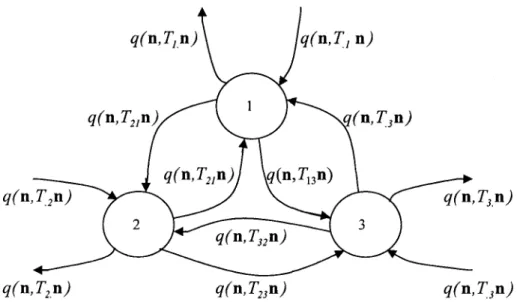
In Figure 2.1 we can see an example of an open migration process with 3 colonies, where an individual can reach some colony from outside the system, leave the system from a colony and move between colonies; the transition rates are also shown in the figure and are given by equations (2.7), (2.8) and (2.9).
q(n,T2n)
q(n,T2n)
Figure 2.1 Transition between colonies in an open migration process
A solution to Equation (2.5) is ax= a2,....-a, =\. Thus nl,n2,...,nj, are
independent and the form of the equilibrium distribution, for each one is a negative binomial distribution, [1], given by
'fj+nj-l
(2.14)
Q. C
where f- = —- and g} = - i - .
c d
The expected number of individuals in group j is given by
a
J
(2.15)
uj ~c.i
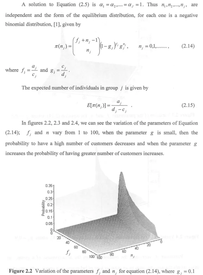
In figures 2.2, 2.3 and 2.4, we can see the variation of the parameters of Equation
(2.14); fj and n vary from 1 to 100, when the parameter g is small, then the
probability to have a high number of customers decreases and when the parameter g
increases the probability of having greater number of customers increases.
0,35- 0.3-
0.25-•f 0.15:
a.
0.1-
0.05-u
o
2 0 ^ 40'
fj
40 2u
100
Figure 2.2 Variation of the parameters fj and nj for equation (2.14), where g. =0.1
Figure 2.3 Variation of the parameters /; and «y for equation (2.14), where g f =0.5
Figure 2.4 Variation of the parameters /; and nj for equation (2.14), where g; =0.9
Parameter f} represents the relation between the attractiveness of a group, in
other words the attractiveness to an outsider user of belonging to a group, with respect to the attractiveness to an outsider of an individual in a group, if this parameter increases
then the probability of belonging to a group increases too. The parameter gf represents
the relation between the attractiveness to an outsider of individual in a group with respect to the propensity to depart from the group; in other words, it represents the relation between the arrivals with respect to the departures of a colony.
2.3.2 Closed Migration Processes
Now, we apply the general concept of closed migration processes described in Section 2.1, to the social grouping behavior, and obtain the system's behavior; where the total number of users in the system is fixed and no one can enter or leave the system from or to the outside. Thus, if we consider a closed migration process with the transition rates given in Equation (2.9), where
t(nj) = djtij , y/k(nk) = ak+cknk,
ak,ck,dk >0,
and the total number of customers in the system is N; the form of the equilibrium distribution is obtained by using Theorem 2.1, nevertheless the constant B is in general an awkward expression; it is simplified when Cj Id;. = g for j - l,2,....J.
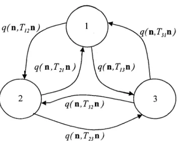
In Figure 2.5 we can see and example of a closed migration process with 3 colonies, where an individual can only move between colonies, here it is not possible to reach some colony from the outside of the system or leave the system from some colony; the transition rates are given by Equation (2.9).
Then, the equilibrium distribution for this closed migration process is given by
(
J
V
*(n) = w *
t l \
J
\
(
2
-
16
)
V J
J a.
for n such that ^ rij = N and /y = — .
7=1 ' C
7
q(n,Tl2n) g(n,T 3ln)
q(n,T23n)
Figure 2.5 Transition between colonies in an closed migration process
The marginal distribution for nj is the Polya's distributional].
—
V ./
k=\
N \
r
)
1
(- 1
u /
/
V
J f • ~ / f
k=\
N-nj
(2.17)
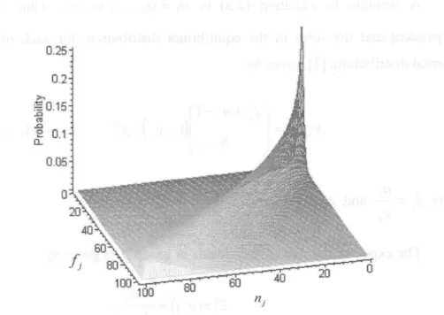
In Figure 2.6, we can see the variation of the parameters of Equations (2.17); /
varies from 0 to 80 and n varies from 0 to 40. Notice that when the parameter / is
increasing, the probability to have a high number of customers increases as well.
Figure 2.6 Variation of the parameters f} and rij for equation (2.17)
2.4 Polya's Urn Scheme
There is a similitude between a social grouping behaviour in its closed form and the Polya's urn scheme. The urn is equivalent to the system of social grouping behaviour and the color of the balls of the urn is equivalent to the groups i.e., each group represents a color. Thus, Polya's urn can help us to understand the parameters of social grouping behavior in its closed form.
An urn contains b black balls and w white balls, a ball is drawn at random, and it is replaced and c balls of the same color are added. A new drawing is made from the urn replacing and adding more balls, and this procedure is repeated, [4].
Now, we can consider two geographical areas A and B as an urn where there are b black balls in A and w white balls in B, in this case b and w can represent the attraction level of the geographical area to an individual; we can set the initial proportion of black and white balls in order to characterize geographical areas and to adjust the initial probabilities to some convenient value. We draw a ball from the urn, then if it is black or white ball, we replace and add in c more attractiveness units of the same color.
Repeating this procedure, we can obtain the probability that in N = nx+n2
drawings, the first nx ones result in black balls and the remaining n2 ones result in white
balls as follows,
b (b + c) (b + 2c) (b + nxc-c) w
(b + w) (b + w + c) (b + w+2c) (b + w + nxc-c) (b + w + nxc-c)
(w + c) (w + 2c) (w + nxc-c) (2.18)
(b
(b+w+Nc-c)
If we consider any other ordering of nx black balls and n2 white balls, to
calculate the probability we will obtain the same probability as that given in (2.18), but
rearranged in a new order. It follows that all possible combinations of «, black and n2
white balls have probabilities given by Equation (2.18); and to obtain the probability Pn n
that n drawings result in nx black and n2 white balls in any order we must multiply
n
Equation (2.18) by , obtaining the number of possible orderings. Then we have a
V)
new expression for this probability, [4], given by
(—blcY—wlc
j v "i A n2 j
w)/c
N N
we can see «, and n2 as the number of individuals in location areas A and B.
2.5 System Performance
In the design of a cellular system, it is very important to define its optimal configuration; to reach a good efficiency. The grade of service GoS is an important parameter to evaluate the system and it is defined as the number of unsuccessful calls relative to the total number of attempted calls. In practice we can express it as the proportion of calls that are blocked during the busiest hour and it is directly related to the blocking probability. Cellular systems are designed to have a GoS of 2%, rising up to 5% as the system grows.
2.5.1 Blocking Probability
The blocking probability determines the proportion of calls that are rejected or will not obtain service from the system; generally we can use the Erlang B formula to calculate this probability, it is based on a Markov chain model; we use the following assumptions.
• Call request are memoryless, implying that all users, including blocked users, may request a channel at any time.
• All free channels are fully available for servicing calls until all channels are occupied.
• The probability distribution of channel holding time is exponential. • There is a finite number of channels available.
• The number of subscribers is assumed to be infinite. • Traffic requests are described by a Poisson process. • Interarrival times of calls are independent of each other
The arrival rate, At, is independent of the state, then Af = A; the departure rate,
jui, is state dependent; the expression for the Erlang B formula is:
(2.20)
where A is the traffic intensity in erlangs, and C is the total number of available channels in the system.
In systems with a small number of users, the Erlang B is not a good formula to calculate the blocking probability; in such case the Engset formula can be used; the
assumptions to Engset are same as those of the Erlang B with the exception that the number of users is finite, then in the Engset model the arrival rate, At, is dependent on
the state; in this model A, =(N - i)A; the expression for the Engset formula is,
B(N,A,C)= ;
C,{,,
, (2.21)
where A is the traffic intensity in erlangs, C is the total number of available channels in the system, and N >C is the total number of subscribers in the system.
Some systems can be modeled by an M/M/co queue, which has a Poisson
e'AA"
stationary distribution, then the probability of having n subscribers is P = , thus, n\
we can calculate the blocking probability, with the expression,
where A is the traffic intensity in erlangs, and C is the total number of available channels in the system.
If a system can be model as a queueing network by a closed migration processes, we can calculate the new call blocking probability, with the stationary distribution as we can see in the follow chapter in Section 3.4.
In this Chapter, we described the concepts of user mobility and showed how to consider it for cellular performance evaluation. We develop the model proposed and in the following chapter we use to measure new call blocking in a cellular system.
Chapter 3
Model Description
In this thesis, we are interested in predicting the position and mobility of cellular customers, and determine other parameters like new call blocking probability in a cellular or carrier to interference. In order to do this, we use the concept of social grouping behavior as a closed migration process described in Chapter 2, considering the principal activity centers denominated attractors.
3.1 Attractor Model
We consider a city as a finite associated group of different zones of activity called attractors, where the number of customers is varying with respect to time according to the characteristics of the attractor and its relation with other adjacent attractors.
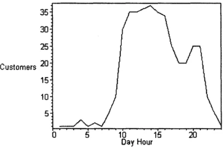
An attractor is an area or region that attracts customers and in which they spend certain time; for example working areas, residential areas, entertainment areas or specifically shopping centers, theaters, and others. Each attractor has different grades of attraction, this grades could change with time depending on the infrastructure characteristics and social events; then each attractor has its own time function as shown in Figure 3.1, where we represent the time function of an industrial area, it is to say the number of customers in the attractor respect the day hour. In Figure 3.2, we can see some kinds of attractors and its interaction between them.
Customers
10 15 Hour
Figure 3.1 Attractor function of an industrial area
Industrial area
'ential area
Entertainment area
Figure 3. 2 Interaction between attractors
This thesis use attractors in a cellular system. A cell can have a finite number of attractors. In order to determine the attractors in a cell, we have to analyze the geographical area, the infrastructure of the zone and the user's customs; as we can see, each cell has a different number and kind of attractors, as shown in Figure 3.3.
*"."**-; s^\;
N i l
IWw:**-Figure 3. 3 Attractors in a specific city's area
In this model, we consider the attractor function referred solely to the characteristics of attraction on the cellular systems' customers. We define an attractor 0, which contains all those customers who are not active in the network, in other words, we consider a set of J attractors, where the active customers move between attractors and the inactive customers are in attractor zero. In each coverage area, it is possible to consider one attractor that contains the dispersed customers in the cell's coverage area, which are not in an specific attractor; the location of this attractor will have to be in a point of balance for these dispersed customers. Considering what has been just discussed, we can represent the system of attractors in a particular cell or group of cells as a closed migration process.
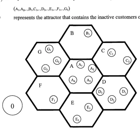
In the model, we will represent the cells and attractors as shown in Figure 3.4., where
represents the cell's name; for example (A,B,C,D,E,F,G)
z represents the attractor in a specific cell where7=1,2,3,...;
0 represents the attractor that contains the inactive customers of the system.
Figure 3. 4 Cells and attractors representation
Each attractor has its own characteristics (as a function of time), and parameters as follows
* ^ . The attractiveness to an outsider customer to belong to group k on time t, that generates a call.
k : The attractiveness to an outsider customer to belong to an individual group
k.
k : The propensity to depart of a customer from group j of an individual
group j , this parameter is the service rate; in this work we assume that is
constant on time.
Jk : Is a measure of the customer's mobility from group j to k; as a function
of time.
J^ ' : Arrival rate, into attractor j as a function of the time.
In Figure 3.5, we can see the representation of one cell with three attractors, their transitions between them and with the attractor zero.
>
Figure 3. 5 Representation of the attractors and their transition
3.2 Mobility
We consider a cellular network where each cell z has z j attractors as shown in Figure
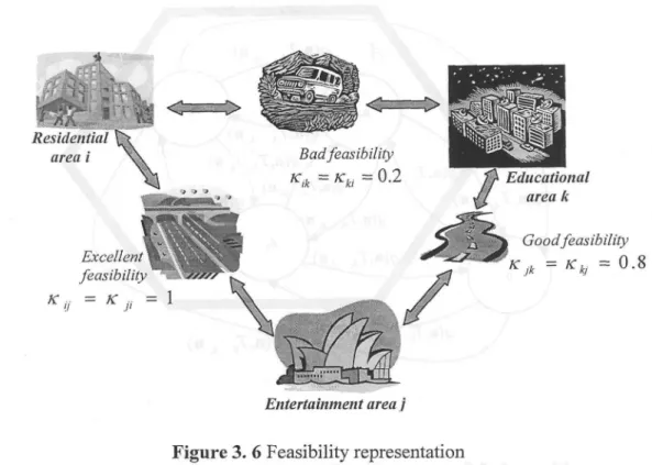
3.4. When an specific attractor increase its level of attraction, the amount of customers that enter to the attractor increase too and the amount of customers that leave of the attractor decrease, in this conditions the proportion of customers who enter and leave to others attractors decrease too; now if the level of the attractor decrease the contrary effect is observed, thus, we can know the attractor characteristics and build the attractor function. We define a parameter K, , (t) as in [2], as the geographical feasibility of the
customer to go from attractor z to attractor zk at time t, as shown in Figure 3.6. This
parameter satisfies the inequality 0 < Kz Zj (/),:£ 1; where, if KZjh (t) is equal to zero, then,
it is not possible to go from Zjto attractor zk and if Kz_Zt(t) is equal to 1, there are not
restrictions to go from attractor z; to attractor zk.
Residential area i
Excellent; feasibility "
= K ,,• =
. Good feasibility
* V = K =0.8
Entertainment area j
Figure 3. 6 Feasibility representation
The value of the feasibility parameter K (t), depends on the zone's
j ft
characteristic, such as the road network, distance between attractors, the day's hour, customers behavior. The evaluation of this parameter can be estimated statistically, studying the zone's characteristics and the flow of customers.
The flow of customers between attractors can be represented by the parameter Kifi)* which is defined as the customer's mobility between attractors z;. and zk,
Xzz it), and is obtained as, [2],
(3-D
where
z; Attractor y in cell z .
nz (t) represents the attraction function, (average number of active customers
in attractor Zj at time t).
X2 (?) is the mobility coefficient from attractor Zj to attractor zk.
K
z.zk (0 is me customers' feasibility, to go from attractor z; to attractor zk.
Then, we can predict the number of active customers in attractor z; at time /,
nz (t), by the equations given in, [2], as follows
0.2)
where
nz(t — 1) average number of active customers in attractor z. at time t-\.
Xz z it) is the mobility coefficient from attractor Zj to attractor zk.
As we can see, the second term on the right hand side of Equation (3.2), represents the active customers, who are going from an attractor z, ± z f to attractor z;;
thus, in order to calculate the number of customers hz {t), who are going from a cell to
another one, we can use
(3.3)
7=1 v, /ez v*z
v*0
We can see Equation (3.3) as the average number of active customers that generate a handoff in cell z at time t.
3.3 Closed Migration Process Model
We can model a cellular system as a closed migration process, as we discussed in Chapter
2. The total number of customers in the system is fixed (N) and it can be calculated from the attractor function of each cell as follows,
(3.4)
thus, the transition rates between attractors are
q(n, T., ri) = X., d7 n. (a, + c. n, ),
" V ' z j2
k ' 2 jz
k z ) z
j V z k z
k z k '
(3-5)
where a, ,cz ,d2 > 0 , and the equilibrium distribution for the system is the Polya's
distribution given by
-IX,
zi
N ^~1
n
(3.6)azz
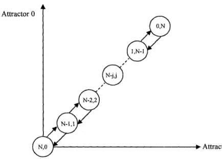
where fz = —-; and the number of system's states (nss) can be calculated by the relation
nss =
to-1 (3.7)
where ta is the total number of attractors in the system. For example if we have a system with two attractors we will have the states, as shown in Figure 3.6. ; if ta = 2 then
nss = N +1
Attractor 0
-••Attractor A,
Figure 3. 7 states for two attractors
3.3.1 Determination of parameters
In order to know the parameters az and c2 in Equation (3.5), we can analyze the system
as a Polya's urn, as we saw in Chapter 2. The parameter az is similar to b and w balls in
Equation (2.19), where b and w represent the initial number of black and white balls. In our model, it is equivalent to the initial value of the attractiveness to an outside customer to belong to group k. In other words the initial attraction value; the parameter c, can be
seen as c in Equation (2.19), where c represents the number of balls of same color b or w which are added after we draw a ball from the urn. Then, our model is equivalent to the increment of attractiveness to an outsider to belong to an individual group k, whenever
an attractor increases its number of active customers, i.e., when a customer makes a call. We can summarize this in the Table 3.1.
Table 3.1 Parameters equivalent between Polya's urn and Closed Migration Processes
Polya's urn
b or w. initial balls
c increment of balls b or w, when we draw a ball from the urn.
Closed Migration Processes
az initial attractiveness
cz attractor's attractiveness increment
when a customer makes a call.
In this work, the service rate is exponentially distributed with parameter dz for
attractor z.. Each attractor has the same dz . If we take the condition of Equation (2.16),
where cz I dr = g , i.e., we assume that c2 is also constant.
j Z j j
By the simulation of the model, we determinate some optimums values to the
model application; thus, is recommendable to maintain constant in the time the f0 value,
having to be much greater than the values of attraction of the other attractors, since the time that a user remains inactive is greater to the time than he remains active; being recommendable f0 - N; other important condition is the relation between fz and the
traffic (erlangs), we determinate, fz , increasing or decreasing in order to condition, 0.8
units of fz by 1 erlang.
3.4 Performance Evaluation
In this model we measure performance evaluation at a cell level given by new call blocking probability. This measure can be obtained using the stationary distribution in
Equation (3.6), for the possible states in each cell; then if we have z cells with mz
channels of capacity, the new call blocking probability in cell z will be given by
I ^ 1 (3.8)
n : ^ [ J
where Bz Blocking probability of cell z, n, total active customers in cell z, mz
capacity of cell z, n vector n = (na,nA>,nAi ,...,nFj ,...,nZj).
Since we are not using any strategy to provide priority to handoff calls over new calls, Equation (3.8) also gives the handoff blocking probability.
Chapter 4
Numerical Results
This chapter presents a proposed algorithm to determine the mobility and the system's performance; according to the model introduced in Chapter 3. We present numerical results of two proposed scenarios.
4.1 Proposed algorithm
We propose the following algorithm in Figure 4.1, as follows
1. The first step is to determine the system's characteristics, as geographical location, number of cells, capacity of each cell.
2. Determine the kind, number, characteristics and distribution of attractors in the system.
3. Determine the attractor functions, nz{t), referred to the attraction's
characteristics on the customers' system.
4. Calculate the total number of customers N in the system by Equation (3.4).
5. Calculate the mobility coefficient A,2.2(f) for each pair of attractors, using
Equation (3.1).
6. Now, we calculate the number of active customers moving between cells h, (t), by
Equation (3.3), this is equivalent to the handoffs in each cell.
Determine [System's characteristics]
(Geographical location, number of cells, capacity of each cell)
Find [attractors]
(Kind, number, characteristics and distribution)
Find«z.(0
[attractors' function]
(on the customers' svxterrA
no
yes
Find [N\
Equation (3.3)
Equation (3.1)
Predict [ nz( 0 l
Equation (3.2)
Determine
[attractor's parameters]
Find
[New call Blocking Probability]
Equation (3.8)
Find [ h2 (t) ]
Equation (3.3)
Figure 4.1 Block diagram of proposed algorithm
7. With Xzlk it), we can predict the number of active attractor's customers nz (t),
by Equation (3.2).
8. In order to evaluate the system's performance, we have to determine the attractors' parameters; aZk ,cZt ,d,t ,fZk, considering the conditions
• aXt,cZt,dIt>0
• dz = d is the service rate and it's the same for all the cells
• cZk I dZk = cZt I d = g then cZt = c, is constant.
• fz = az I c, the optimal value of fQ is N.
• Equivalency between erlangs and fz , by each increment of traffic of one
erlang, we increment in 0.8 units fz .
9. Now, calculate the new call blocking probability using Equation (3.8).
4.1.1 Scenario 1
The first scenario, is shown in Figure 4.2. We have one cell with one attractor for active customers, and 1000 total customers. Therefore, we have a system with one cell,
J V = 1 0 0 0 and two attractors. The system's behavior and the performance (New call
Blocking Probability) is calculated and compared with the Erlang B, the Engset and the Poisson blocking equations given in (2.20), (2.21), and (2.22), respectively. We define the capacity in channels of cell A as CA. The parameters used in this first scenario are summarized in Table 4.1.
Table 4.1 Parameters of first scenario
N = 1000 customers ta - 2 attractors
nss =1001 states
d = 1 service rate
c = 1 attraction increment
fA> is increasing in order to the erlangs increments. (0.8 units of fAi by 1 erlang )
Figure 4. 2 First scenario
D.1-F
3
A B
B 7
0
Figure 4. 3 New Call Blocking Probability for C^ = 10, TV = 1000, ta = 2
D.1
D.DB-
0.06-BA •
0.04-
0.02-Engset Polya
2 4
Erlang B
B 10 12 14 Erlangs
1B 18
Figure 4. 4 New Call Blocking Probability for CA = 20, N = 1000, ta = 2
Erlangs
Figure 4. 5 New Call Blocking Probability for CA = 30, iV = 1000, ta = 2
Figures 4.3, 4.4 and 4.5, show the new call blocking probability versus traffic in erlangs; for 10, 20 and 30 channels of capacity in the cell respectively. Traffic from 0 to 30 erlangs and N =1000. We can see the behavior of the proposed model compared to the Erlang B, the Engset and the Poisson blocking models. The model has a similar behavior to the Erlang B blocking model.
Polya
BA
10
Erfangs 3Q
40 3026
10 20 ""'Capacity
Figure 4. 6 New Call Blocking Probability using Polya model for N = 100, ta = 2, CA = 0 to 30, traffic 0 to 40 erlangs.
Erlang B
10
Erlangs20 Capacity
Figure 4. 7 New Call Blocking Probability using Erlang B model for N = 100, ta = 2, CA = 0 to 30, traffic 0 to 40 erlangs.
Engsst
•»•--?•**••*»•""*•>»})»«$«,(.,;. ,
Erfangs Capacity
Figure 4. 8 New Call Blocking Probability using Engset model for JV = 100, ta = 2, CA = 0 to 30, traffic 0 to 40 erlangs.
Poisson
Capacity
Figure 4. 9 New Call Blocking Probability using Poisson model for iV = 100, ta - 2, CA = 0 to 30, traffic 0 to 40 erlangs.
Figures 4.6, 4.7, 4.8 and 4.9, show the behavior of the model proposed, for the Polya, the Erlang B, the Engset and the Poisson blocking models, respectively. Total
customers are 100 and the traffic was varied from 0 to 40 erlangs and capacity from 0 to 30 channels. Our model has a similar behavior than the Erlang B blocking model.
4.1.2 Scenario 2
The second scenario is shown in Figure 4.10. Several attraction areas in an urban region
are specified, each one with different attraction function as shown in Figure 4.11. In this Figure 4.10, we can see a system of two cells, in cell A there are two attractors Ay,A2
with different characteristics and in cell D there is one attractor Dy, the transitions rates
are specified between attractors and with the attractor zero. Thus, we proceed according to the proposed algorithm, as follows
Figure 4.10 Second scenario
System's characteristics: The number of cells is 2 cells.
Total system states is 2925 obtained using Equation (3.7). The remaining parameters are in Table 4.2
Table 4. 2 System's characteristics
Characteristics
Capacity (channels)
Offered Traffic by customers (erlangs) Attractors
Kind
Attractor function
Cell A
2 0.025
A
Working area Residential Area nAl(t)Cell D
2 0.025
A
Entertainment Area S3B
|
| 12 1D B- 4-Working area \D
1D
15 2DHours of the day
Figure 4.11 Attractor function, working nA (t), residential nA (t), entertainment nD (t)
• Using Equation (3.4) on attractors' function shown in Figure 4.11, we calculate N=24 customers in the system. Now, we calculate the mobility coefficient
X...k(t), by Equation (3.1); Table 4.3, shows the values of A:. (t), for some
hours of the day; in this second scenario. The feasibility between attractors, k, is assumed to be one.
Table 4. 3 Mobility coefficient between
Time: 1 a.m.
attractors for some hours on the day
Time: 8 a.m.
A 0
A
A
A
0 0.000 0.875 0.875 0.875A
0.042 0.000 0.042 0.042A
0.042 0.042 0.000 0.042A
0.042 0.042 0.042 0.000 X 0A
A
A
0 0.000 0.708 0.708 0.708A
0.208 0.000 0.208 0.208A
0.042 0.042 0.000 0.042A
0.042 0.042 0.042 0.000Time : 11 a.m. Time: 4 p.m.
X 0
A
A
A
0 0.000 0.083 0.083 0.083A
0.500 0.000 0.500 0.500A
0.208 0.208 0.000 0.208A
0.208 0.208 0.208 0.000 X 0A
A
A
0 0.000 0.417 0.417 0.417A
0.292 0.000 0.292 0.292A
0.042 0.042 0.000 0.042A
0.250 0.250 0.250 0.000 A 0A
A
A
Time: 8 p 0 0.000 0.083 0.083 0.083
A
0.542 0.000 0.542 0.542 .m.A
0.167 0.167 0.000 0.167A
0.208 0.208 0.208 0.000 A 0A
A
A
Time: 111 0 0.000 0.667 0.667 0.667A
0.083 0.000 0.083 0.083 a.m.A
0.042 0.042 0.000 0.042A
0.208 0.208 0.208 0.000To determine the number of active customers moving between attractors, we use Equation (3.3). Table 4.2 shows the result by the hour of the day.
Table 4. 4 Active customers moving between attractors by the hour of the day.
Cell A
Cell D
Cell A
Cell D
14 3 3 15 3 6 16 2 4 17 1 1 18 2 1 19 4 1 20 1 3 21 3 4 22 3 5 23 1 3 24 0 0
The results in Table 4.4, can be seen as the numbers of handoffs in each cell by the hour of the day. These values increase when mobility increases.
To evaluate the system's performance, we determine the attractors' parameters
using d = 1, c - 1, and /0 =24, fAi,fAi,fDi increasing or decreasing in order to
condition, 0.8 units of fz by 1 erlang. For example, if we have 0.75 erlangs, we
increase fz in 0.75 x 0.8 = 0.6. In Table 4.5, and in Figure 4.12, we can see the
variation by hour of the day of the parameter / for each attractor
(/o'IA\ >//i2'/D, ) ' m t n e s a m e form m Table 4.6, and in Figure 4.13, we can see
the variation by hour of the day of the traffic in erlangs for each attractor.
Table 4. 5 f0, fA, variations by the hour of the day
/ o
A
17 24 0.04 0.02 0.06 18 24 0.2 0.04 0.12 19 24 0.24 0.08 0.04 20 24 0.26 0.08 0.1 21 24 0.26 0.06 0.12 22 24 0.2 0.04 0.14 23 24 0.04 0.02 0.1 24 24 0.02 0.02 0.06 0.25- 0.2- 0.1-0.05:0 1D 15 2D
Hours of the day
Figure 4.12 ,fD variations by the hour of the day
Table 4.6 AX,A2,DX, traffic variation by the hour of the day, in erlangs
Traffic Ax
Traffic A2
Traffic DY
Traffic Ax
Traffic A2
Traffic Dj
Traffic Ax
Traffic A2
Traffic D, 9 0.175 0.025 0.025 17 0.050 0.025 0.075 10 0.300 0.100 0.075 18 0.250 0.050 0.150 11 0.300 0.125 0.125 19 0.300 0.100 0.050 12 0.300 0.125 0.075 20 0.325 0.100 0.125 13 0.325 0.175 0.075 21 0.325 0.075 0.150 14 0.300 0.200 0.100 22 0.250 0.050 0.175 15 0.275 0.150 0.175 23 0.050 0.025 0.125 16 0.175 0.025 0.150 24 0.025 0.025 0.075
M
A
/ V
10 15 20
Hours of the day
Figure 4.13 Ai,A2,Dl, traffic variation by the hour of the day, in erlangs
Finally, we calculate the New Call Blocking Probability for each cell by the hour of a day as shown in Table 4.7, and Figures 4.14 and 4.15.
Table 4. 7 New Call Blocking Probability in percentage for each cell by the hour of a day Time 1 2 3 4 5 6 7 8 9 10 11 12 13 14 15 16 17 18 19 20 21 22 23 24 Polya 0.5422 0.5422 0.5422 0.5422 0.5422 0.8283 0.5422 1.7449 2.4037^ 5.3864 5.7822 5.7991 7.0862 7.0759 5.7653 2.3855 0.8257 3.8036 5.3944 5.7822 5.3627 3.7980 0.8232 0.5406 Cell Erlang B 0.1189 0.1189 0.1189 0.1189 0.1189 0.2609 0.1189 0.9688 1.6393 5.4054 5.9600 5.9600 7.6923 7.6923 5.9600 1.6393 0.2609 3.3457 5.4054 5.9600 5.4054 3.3457 0.2609 0.1189
A
Engset 23.8754 23.8754 23.8754 23.8754 23.8754 35.6692 23.8754 57.4468 65.5582 80.6428 81.6551 81.6551 84.1463 84.1463 81.6551 65.5582 35.6692 75.1816 80.6428 81.6551 80.6428 75.1816 35.6692 23.8754 Poisson 0.0020 0.0020 0.0020 0.0020 0.0020 0.0066 0.0020 0.0503 0.1148 0.7926 0.9334 0.9334 1.4388 1.4388 0.9334 0.1148 0.0066 0.3599 0.7926 0.9334 0.7926 0.3599 0.0066 0.0020 Polya 0.1329 0.1329 0.1329 0.1329 0.1329 0.1326 0.1329 0.1320 0.1316 0.4046 0.6975 0.4040 0.4022 0.5459 1.0099 0.8632 0.4129 0.8579 0.2649 0.6975 0.8527 1.0176 0.7127 0.4135 Cell Erlang B 0.0305 0.0305 0.0305 0.0305 0.0305 0.0305 0.0305 0.0305 0.0305 0.2609 0.6897 0.2609 0.2609 0.4525 1.2864 0.9688 0.2609 0.9688 0.1189 0.6897 0.9688 1.2864 0.6897 0.2609B
Engset 9.7320 9.7320 9.7320 9.7320 9.7320 9.7320 9.7320 9.7320 9.7320 35.6692 51.8797 35.6692 35.6692 44.8052 61.9117 57.4468 35.6692 57.4468 23.8754 51.8797 57.4468 61.9117 51.8797 35.6692 Poisson 0.0003 0.0003 0.0003 0.0003 0.0003 0.0003 0.0003 0.0003 0.0003 0.0066 0.0296 0.0066 0.0066 0.0155 0.0784 0.0503 0.0066 0.0503 0.0020 0.0296 0.0503 0.0784 0.0296 0.0066The behavior of the proposed model is similar to that of the Erlang B, nevertheless our model has a better behavior when the traffic is increased, this can be seen in Figures 4.14 and 4.15.
D.
D
D
D
*
t \B-
6-
4-
2-
D-fP
i
A f / \ jj * 0 5
/
i
i / it. ^ Engset1D
\
^\
15
s. I \ \\i
r'
ij
fr~"~~ "<
* ^ 1 "l 1 1 1 1 \ \
2D
1D 15
Hours of the day
O.DB-
D.D4-
D.D2-10 15
Hours of the day
20
Figure 4.14 New Call Blocking Probability variation in cell A by the hour of a day, iV=24, CA=2, taA=2
10 15
Hours of the day
20
10 15
Hours of the day
20
Figure 4.15 New Call Blocking Probability variation in cell D by the hour of a day,
iV=24, CD=2, taD=\
Chapter 5
Conclusions and Further Research
In this Chapter in section 5.1 we present the conclusions of the thesis. In section 5.2 some future research are presented.
5.1 Conclusions
The limited resources and the increase in the demand of resources of the PCS' system have generated the necessity to investigate the patterns of mobility of the users within the system. The analysis of mobility is a excellent tool to design the mobile communications systems, it is very important for the efficient administration of the resources of the system and obtain a good performance of quality of service.
On Chapter 3 we presented a new method to analyzed the performance of the PCS' system. This model consider the characteristics of customers mobility and the characteristics of the geographical zone using the concept of attractor where the number of customers is finite and it is analyzed as a Migration Processes by the concept of Social Grouping Behavior.
The model is based in the attractor concept, and Social Grouping Behavior to apply it in a real system, first we have to analyze the statistical information and the characteristics of the geographical zone, in which our system is it, it to determine the
level of the relation of attraction of each attractor. The main aspect to obtain is the attractor function from as we can calculate the necessary parameters for our model.
The result of the thesis indicate that the model proposed have a similar performance than the Erlang B blocking probability model. In our model the total number of customers in the system is finite, the arrival rate is state dependent, in other words, the more customers that are free to generate a call the greater that arrival rate.
In the system design is very important pay attention in the location of the cells and the distribution of resources respect the number and characteristics of the attractors, greater amount of attractors and greater attraction level, then greater new call blocking probability.
5.2 Further Research
According to the work done in this thesis, the following ideas can be suggested for further research.
• The use of the migration process as a Social Grouping Behavior in its closed form can be extended to consider power controlled systems as a CDMA wireless network.
• Using strategies to provide priority to handoff calls over new calls, we could analyze the model proposed to determine a Equation to give the handoff blocking probability.
• It is possible to use the migration process as a Social Grouping Behavior in its open form.
• Continuing the work under consideration of a process in which customers form themselves into clusters, then, it is possible to apply the Clustering Processes.
The application of the proposed model has a complexity to determine all possible states, in such reason, the design and construction of a data base, that maintains the information of all the possible states and their probabilities with respect to the attractor function can be a solution, this data base will have to be updated periodically.
Determine a procedure to calculate the relation between fo,fz,,N and the
traffic in Erlangs, in order to adjust these parameters to the characteristics of the system.
References
[1 ] F.P. Kelly, Reversibility and Stochastic Networks, John Wiley & Sons Ltd, 1987
[2] J.I. Bermudez Vasquez, "Analysis and modeling of the population distribution for cellular systems," M.Sc. in EE. Thesis, ITESM June 1997
[3] Esteban A. Carrasco Melendez, "Using the diffusion and the attractor models to represent traffic intensity, mobility and interference in a power controlled system,"MSc. in EE. Thesis, ITESM July 2001
[4] W. Feller, An Introduction to Probability Theory and Its Applications. John Wiley & Sons Third Edition. 1968.
[5] J. Markoulidakis, G. Lyberopoulos, D. Tsirkas, E. Sykas, "Mobility Modeling in Third-Generation Mobile Telecommunications Systems," IEEE Personal Communications magazine, vol. 4, No. 4 pp. 41-56, August 1997.
[6] Christopher Rose and Roy D. Yates, "Location Uncertainty in Mobile Networks: A Theoretical Framework," IEEE Communications Magazine, vol. 35, No. 2 pp. 94-101, February 1997.