Methodology of Diagnostic Tests in Hepatology
Erik Christensen** Departament of medical endocrinology and gastroenterology I, Bispebjerg Hospital, University of Copenhagen, Denmark.
ABSTRACT
The performance of diagnostic tests can be assessed by a number of methods. These include sensitivity, specificity, positive and negative predictive values, likelihood ratios and receiver operating characteristic (ROC) curves. This pa-per describes the methods and explains which information they provide. Sensitivity and specificity provides measures of the diagnostic accuracy of a test in diagnosing the condition. The positive and negative predictive values estimate the probability of the condition from the test-outcome and the conditions prevalence. The likelihood ratios bring to-gether sensitivity and specificity and can be combined with the conditions pre-test prevalence to estimate the post-test probability of the condition. The ROC curve is obtained by calculating the sensitivity and specificity of a quantitative test at every possible cut-off point between normal and abnormal and plotting sensitivity as a func-tion of 1specificity. The ROC-curve can be used to define optimal cut-off values for a test, to assess the diagnostic accuracy of the test, and to compare the usefulness of different tests in the same patients. Under certain conditions it may be possible to utilize a tests quantitative information as such (without dichotomization) to yield diagnostic evidence in proportion to the actual test value. By combining more diagnostic tests in multivariate models the diag-nostic accuracy may be markedly improved.
Key words. Diagnostic test. Sensitivity. Specificity. Positive predictive value. Negative predictive value. Likelihood ra-tio. Receiver operating characteristic curve. ROC curve.
Correspondence and reprint request: Erik Christensen, MD, Dr. Med. Sci. Chief Consultant Physician, Associate Professor
Department of Medical Endocrinology and Gastroenterology I, Bispebjerg Hospital,
Bispebjerg Bakke 23
DK-2400 Copenhagen NV, Denmark Email: [email protected]
Manuscript received: August 2, 2009. Manuscript accepted: August 2, 2009. INTRODUCTION
The performance of diagnostic tests can be asses-sed by a number of methods developed to ensure the optimal utilization of the information provided by symptoms, signs and investigational tests of any kind for the benefit of the patient. The evaluations of diagnostic tests include sensitivity, specificity, po-sitive and negative predictive values, likelihood ra-tios and ROC-curves.1 This article will review these
methods and provide some suggestions for their ex-tension and improvement. The methods will be illus-trated by an important variable in hepatology, namely the hepatic venous pressure gradient (HVPG).
The decision of the doctor in regard to diagnosis and therapy is based on the variables characterising
the patient. It is therefore essential for the doctor: a) to know which variables hold the most informa-tion and b) to be able to interpret the informainforma-tion in the best possible way.1 How this is done depends on
the type of the variable and on the type of decision, which has to be made. Some descriptive variables are by nature dichotomous or binary like variceal bleeding being either present or absent. However, many variables like liver function tests and the he-patic venous pressure gradient (HVPG) are measu-red on a continuous scale, i.e. they are quantitative variables.
A doctor’s decision has to be binary, i.e. yes or no concerning a specific diagnosis and treatment. The-refore, for a the simple diagnostic tests to provide a yes or no answer, quantitative variables need to be made binary by introducing a threshold or cut-off le-vel to distinguish between ‘normal’ and ‘abnormal’ values.
CLASSIFICATION OF NORMAL AND ABNORMAL
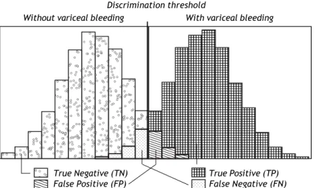
causes some patients to be misclassified. The larger the overlap, the poorer the discrimination of the test and the larger the proportion of misclassified patients. This is illustrated in figure 1. Patients with the condition in question (here variceal blee-ding) could have a positive test (here hepatic venous pressure gradient (HVPG) above 12 mm Hg). They would be the True Positives (TP). But some pa-tients with the condition could have a negative test i.e. an HPVG below 12 mm Hg. They would be the
False Negatives (FN). In patients without
the condition, the test would frequently be negative i.e. the HVPG would be below 12 mm Hg. That would
the True Negatives (TN). But some patients
without the condition could have a positive test i.e. an HVPG above 12 Hg. That would be the False Positives (FP). The false negatives and the
fal-Table 1. Test classification of patients summarized in a 2 x 2 table. The example shows the relation between high (≥ 12 mm Hg) or low (< 12 mm Hg) Hepatic Venous Pressure Gradient (HVPG) and occurrence of vari-ceal bleeding.
HVPG Bleeding No bleeding
High True Positive (TP)* False Positive (FP)** Low False Negative (FN)** True Negative (TN)*
*Agreement between test and patient outcome (True Positive and True Ne-gative). ** Disagreement between test and patient outcome (False Positive and False Negative).
Table 2. Various measures of performance of a binary classification test. In this table the example presented in table 1 is supplemented by the definition and calculation of sensitivity (true positive rate ), false positive rate, positive likelihood ratio (*), specificity (true negative rate), false negative rate, negative likelihood ratio (**), positive predictive value and negative predictive value.
HVPG Bleeding No bleeding
High True Positive (TP) = 70 False Positive (FP) = 30 Positive predictive value = TP/(TP+FP) = 70/(70+30) = 0.70 Low False Negative (FN) = 6 True Negative (TN) = 194 Negative predictive value =
TN/(FN+TN) = 194/(6+194) = 0.97
True Positive rate* = True Negative rate** = Positive likelihood ratio* =
Sensitivity* = Specificity** = TP-rate/FP-rate = 0.92/0.13 = 7.1* TP/(TP+FN) = 70/(70+6) = 0.92* TN/(FP+TN) = 194/(30+194) = 0.87**
False negative rate** = False positive rate* = Negative likelihood ratio** =
FN/(TP+FN) = 6/(70+6) = 0.08** FP/(FP+TN) = 30/(30+194) = 0.13* FN-rate/TN-rate = 0.08/0.87 = 0.09**
Figure 1. Schematic illustration of the dis-tribution of HVPG (hepatic venous pressure gra-dient) in patients without variceal bleeding and in patients with variceal bleeding. Since the distributions overlap, the HVPG does not provi-de complete discrimination between bleeding and non-bleeding patients. For most of the pa-tients with variceal bleeding the HVPG would be above the discrimination threshold (usually 12 mm Hg); they would be classified as True Posi-tives (TP). However, some patients with vari-ceal bleeding would have HVPG below the discrimination threshold; they would be classi-fied as False Negatives (FN). For most of the Discrimination threshold
True Negative (TN) True Positive (TP) False Positive (FP) False Negative (FN)
patients without variceal bleeding the HVPG would be below the discrimination threshold of 12 mm Hg; they would be classified as
True Negatives (TN). However, some patients without variceal bleeding would have HVPG above the discrimination threshold; they would be classified as False Positives (FP).
se positives are the patients who are misclassified. An effective diagnostic test would only misclassify few patients.
The classification of the patients by the test can be summarized in a 2 x 2 table as shown in table 1.
aaaaaa aaaaaa aaaaaa aaaaaa aaaaaa aaaaaa aaaaaa aaaaaa aaaaaa aaaaaa aaaaaa aaaaaa aaaaaa aaaaaa aaaaaa aaaaaa aaaaaa aaaaaa aaaaaa aaaaaa aaaaaa aaaaaa aaaaaa aaaaaa aaaaaa aaaaaa aaaaaa aaaaaa aaaaaa aaaaaa aaaaaa aaaaaa aaaaaa aaaaaa aaaaaa aaaaaa aaaaaa aaaaaa aaaaaa aaaaaa aaaaaa aaaaaa aaaaaa aaaaaa aaaaaa aaaaaa aaaaaa aaaaaa aaaaaa aaaaaa aaaaaa aaaaaa aaaaaa aaaaaa aaaaaa aaaaaa aaaaaa aaaaaa aaaaaa aaaaaa aaaaaa aaaaaa aaaaaa aaaaaa aaaaaa aaaaaa aaaaaa aaaaaa aaaaaa aaaaaa aaaaaa aaaaaa aaaaaa aaaaaa aaaaaa aaaaaa aaaaaa aaaaaa aaaaaa aaaaaa aaaaaa aaaaaa aaaaaa aaaaaa aaaaaa aaaaaa aaaaaa aaaaaa aaaaaa aaaaaa aaaaaa aaaaaa aaaaaa aaaaaa aaaaaa aaaaaa aaaaaa aaaaaa aaaaaa aaaaaa aaaaaa aaaaaa aaaaaa aaaaaa aaaaaa aaaaaa aaaaaa aaaaaa aaaaaa aaaaaa aaaaaa aaaaaa aaaaaa aaaaaa aaaaaa aaaaaa aaaaaa aaaaaa aaaaaa aaaaaa aaaaaa aaaaaa aaaaaa aaaaaa aaaaaa aaaaaa aaaaaa aaaaaa aaaaaa aaaaaa aaaaaa aaaaaa aaaaaa aaaaaa aaaaaa aaaaaa aaaaaa aaaaaa aaaaaa aaaaaa aaaaaa aaaaaa aaaaaa aaaaaa aaaaaa aaaaaa aaaaaa aaaaaa aaaaaa aaaaaa aaaaaa aaaaaa aaaaaa aaaaaa aaaaaa aaaaaa aaaaaa aaaaaa aaaaaa aaaaaa aaaaaa aaaaaa aaaaaa aaaaaa aaaaaa aaaaaa aaaaaa aaaaaa aaaaaa aaaaaa aaaaaa aaaaaa aaaaaa aaaaaa aaaaaa aaaaaa aaaaaa aaaaaa aaaaaa aaaaaa aaaaaa aaaaaa aaaaaa aaaaaa aaaaaa aaaaaa aaaaaa aaaaaa aaaaaa aaaaaa aaaaaa aaaaaa aaaaaa aaaaaa aaaaaa aaaaaa aaaaaa aaaaaa aaaaaa aaaaaa aaaaaa aaaaaa aaaaaa aaaaaa aaaaaa aaaaaa aaaaaa aaaaaa aaaaaa aaaaaa aaaaaa aaaaaa aaaaaa aaaaaa aaaaaa aaaaaa aaaaaa aaaaaa aaaaaa aaaaaa aaaaaa aaaaaa aaaaaa aaaaaa aaaaaa aaaaaa aaaaaa aaaaaa aaaaaa aaaaaa aaaaaa aaaaaa aaaaaa aaaaaa aaaaaa aaaaaa aaaaaa aaaaaa aaaaaa aaaaaa aaaaaa aaaaaa aaaaaa aaaaaa aaaaaa aaaaaa aaaaaa aaaaaa aaaaaa aaaaaa aaaaaa aaaaaa aaaaaa aaaaaa aaaaaa aaaaaa aaaaaa aaaaaa aaaaaa aaaaaa aaaaaa aaaaaa aaaaaa aaaaaa aaaaaa aaaaaa aaaaaa aaaaaa aaaaaa aaaaaa aaaaaa aaaaaa aaaaaa aaaaaa aaaaaa aaaaaa aaaaaa aaaaaa aaaaaa aaaaaa aaaaaa aaaaaa aaaaaa aaaaaa aaaaaa aaaaaa aaaaaa aaaaaa aaaaaa aaaaaa aaaaaa aaaaaa aaaaaa aaaaaa aaaaaa aaaaaa aaaaaa aaaaaa aaaaaa aaaaaa aaaaaa aaaaaa aaaaaa aaaaaa aaaaaa aaaaaa aaaaaa aaaaaa aaaaaa aaaaaa aaaaaa aaaaaa aaaaaa aaaaaa aaaaaa aaaaaa aaaaaa aaaaaa aaaaaa aaaaaa aaaaaa aaaaaa aaaaaa aaaaaa aaaaaa aaaaaa aaaaaa aaaaaa aaaaaa aaaaaa aaaaaa aaaaaa aaaaaa aaaaaa aaaaaa aaaaaa aaaaaa aaaaaa aaaaaa
SENSITIVITY AND SPECIFICITY
The performance of a binary classification test can be summarized as the sensitivity and specifici-ty2-4 (Table 2).
• The sensitivity measures the proportion of ac-tual positives, which are correctly identified as such. It is also called the true positive rate. In the example in table 2 the sensitivity or true posi-tive rate is the probability of high HVPG in pa-tients with bleeding.
• The specificity measures the proportion of ac-tual negatives, which are correctly identified as such. It is also called the true negative rate. In the example the specificity or true negative rate is the probability of low HVPG in patients with no bleeding.
A sensitivity (true positive rate) of 100% means that the test classifies all patients with the condi-tion correctly. A negative test-result can thus rule out the condition.
A specificity (true negative rate) of 100% means that the test classifies all patients without the dition correctly. A positive test-result can thus con-firm the condition.
Complementary to the sensitivity is the false ne-gative rate, i.e. it is equal to 1 – sensitivity. This is sometimes also called the type 2 error (β), which is the risk of overlooking a positive finding when it is in fact true. In the example used the false negati-ve rate is the probability of bleeding in patients with low HVPG.
Complementary to the specificity is the false po-sitive rate, i.e. it is equal to 1 – specificity. This is sometimes also termed the type 1 error (α), which is the risk of recording a positive finding when it is in fact false. In the example the false positive rate is the probability of no bleeding in patients with high HVPG.
POSITIVE AND
NEGATIVE PREDICTIVE VALUES
The weaknesses of sensitivity and specificity are: a) that they do not take the prevalence of the condi-tion into consideracondi-tion and b) that they just give the probabilities of test-outcomes in patients with or without the condition. The doctor needs the opposi-te information, namely the probabilities of the con-dition in patients with a positive or negative test-outcome, i.e. the positive predictive value and negative predictive value4-5 defined below (Table 2).
• The positive predictive value (PPV) is the proportion of patients with positive test results who are correctly diagnosed as having the condi-tion. It is also called the post-test probability of the condition. In the example the positive predic-tive value (PPV) is the probability of bleeding in patients with high HVPG.
• The negative predictive value (NPV) is the
proportion of patients with negative test results who are correctly diagnosed as not having the condition. In the example the negative predictive value (NPV) is the probability of no bleeding in patients with low HVPG.
Both the positive and negative predictive values depend on the prevalence of the condition with may vary from place to place. This is illustrated in table 3. With decreasing prevalence of the condition the posi-tive predicposi-tive value (PPV) decreases and the negati-ve predictinegati-ve value (NPV) increases - connegati-versely with increasing prevalence of the condition.
LIKELIHOOD RATIO
A newer tool of expressing the strength of a diagnostic test is the likelihood ratio, which incor-porates both the sensitivity and specificity of the test and provides a direct estimate of how much a
Table 3. Example showing the influence of a lower prevalence of variceal bleeding on the positive and negative predictive values. By increasing the pre-valence of bleeding from 25% (upper panel) to 3.3% (lower panel) the positive predictive value (PPV) decreases from 0.70 to 0.19 and the negative predic-tive value (NPV) increases from 0.97 to 0.997.
HVPG Bleeding No bleeding
High TP = 70 FP = 30 Positive predictive value (PPV) = TP/(TP+FP) = 70/(70+30) = 0.70 Low FN = 6 TN = 194 Negative predictive value (NPV) = TN/(FN+TN) = 194/(6+194) = 0.97
test result will change the odds of having the con-dition.6-8
• The likelihood ratio for a positive result (LR+) tells you how much the odds of the con-dition increase when the test is positive.
• The likelihood ratio for a negative result (LR-) tells you how much the odds of the condi-tion decrease when the test is negative.
Table 2 shows how the likelihood ratios are being calculated using our example. The positive likeliho-od ratio (LR+) is the ratio between the true positive rate and the false positive rate. In our example it is the probability of high HVPG among bleeders divi-ded by the probability of high HVPG among non-bleeders.
The negative likelihood ratio (LR-) is the ratio between the false negative rate and the true negati-ve rate. In the example it is the probability of low HVPG among bleeders divided by the probability of low HVPG among non-bleeders.
The advantages of likelihood ratios are:
• That they do not vary in different populations or settings because they are based on ratio of rates. • They can be used directly at the individual level. • They allow the clinician to quantitate the
proba-bility of bleeding for any individual patient. • Their interpretation is intuitive: i.e. the larger
the LR+, the greater the likelihood of bleeding, the smaller the LR-, the lesser the likelihood of bleeding.
Likelihood ratios can be used to calculate the post-test probability of the condition using Bayes’ theorem, which states that the post-test odds equals
the pre-test odds times the likelihood ratio: Post-test odds = pre-test odds × likelihood ratio.7,9
Using our example (Table 2) we can now calcula-te the probability of bleeding with high HVPG using LR+ as follows: The pre-test probability p1 (or pre-valence) of bleeding is 0.25. The pre-test probability
p2(or prevalence) of no bleeding is thus 1-0.25 = 0.75. The pre-test odds of bleeding/no bleeding = p1/
p2 = 0.25/0.75 = 0.34. Since LR+ = 6.9 we can (using Bayes’ theorem) calculate the post-test odds
o1as 0.34 × 6.9 = 2.34. Then we can calculate the
post-test probability of bleeding with a high HVPG as o1/(1+ o1) = 2.34/3.34 = 0.70. Note that this is the same value as the PPV.
Similarly we can calculate the probability of blee-ding with a low HVPG using LR- as follows: As be-fore the pre-test odds of bleeding/no bleeding is 0.34. Since the LR- = 0.09 the post-test odds o2 = 0.34 × 0.09 = 0.03. Then the post-test probability of bleeding with a low HVPG is o2/(1+ o2) = 0.03/ 1.03 = 0.03. Note that this is the same value as 1-NPV. The calculation of post-test probabilities from pre-test probabilities and likelihood-ratios is greatly facilitated using a nomogram.10
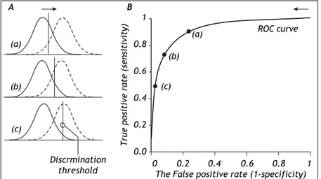
THE ROLE OF THE DISCRIMINATION THRESHOLD
The specification of the discrimination threshold or cut-off is important for the optimal performance of a diagnostic test based on a quantitative variable test like the HVPG. As the position of the threshold changes, the sensitivity and the specificity also change. If you want a high sensitivity (true positive rate), you would specify a relatively low discrimina-tion threshold. If you want a high sensitivity (true negative rate) you would specify a relatively high
Figure 2. The relation between the discri-mination threshold (A) and the position on the receiver operating characteristic (ROC) curve
(B). The ROC curve is a graphical plot of the true positive rate (sensitivity) as a function of the false positive rate (1-specificity) for a diagnostic test as its discrimination threshold is varied through the whole range. By moving the discrimination threshold from left to rig-ht, the points on the ROC curve are obtained from right to left. The figure shows the co-rrespondence between three positions of the discrimination threshold (A) and the three corresponding points on the ROC curve (B).
0 0.2 0.4 0.6 0.8 1
The False positive rate (1-specificity)
True
positive
rate
(sensitivity)
1
0.8
0.6
0.4
0.2
0.0
(a)
(b)
(c) (a)
(b)
(c)
A B
ROC curve
discrimination threshold. The effect of changing the position of the discrimination threshold is illustra-ted in figure 2 (left side) together with the receiver operating characteristic (ROC) curve (Figure 2, right side), which summarizes the overall perfor-mance of a diagnostic test.11-14 The ROC curve
shows the true positive rate (sensitivity) as a func-tion of the false positive rate (1 - specificity) as the discrimination threshold runs through all the possi-ble values.
SEPARATION BETWEEN
POSITIVE AND NEGATIVE TEST VALUES
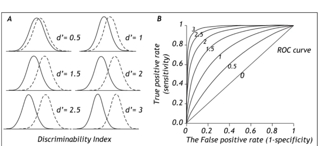
The degree of separation between two distributio-ns is given by the discriminability index d’, whi-ch is the difference in means of the two distributions divided by their standard deviation.15 Figure 3
shows that with increasing separation (decreased overlap) between the distributions the discriminabi-lity index increases (Figure 3, left side) and the middle of the ROC curve moves up toward the upper left corner of the graph (Figure 3, right side). For the discriminability index to be valid, the distribu-tions need to be normal with similar standard de-viations. In practice these requirements may not always be fulfilled.
The area under the ROC curve (AUC) or
c-statistic is another measure of how well a diagnos-tic test performs (Figure 4).11-14 With increasing
discrimination between the test distributions for pa-tients with and without the condition, the AUC or c-statistic will increase. An AUC of 0.5 means no discrimination, an AUC = 1 means perfect discrimi-nation. Most frequently the AUC or c-statistic would lie in the interval 0.7-0.8. The standard error of an AUC can be calculated and ROC-curves for di-fferent diagnostic tests derived from the same pa-tients can be compared statistically.16-18 In this way
the test with the highest diagnostic accuracy in the patients can be found.
The ROC-curve can also be used to define the op-timal cut-off value for a test by localizing the value where the overall misclassification (false positive rate plus false negative rate) is minimum. This will usually be the cut-off value corresponding to the po-int of the ROC curve, which is closest to upper left corner of the plot (i.e. point [0, 1]).
The performance of diagnostic tests may be im-proved if ‘noise’ in the measurement of the diagnos-tic variable e.g. HVPG can be reduced as much as possible. Therefore every effort should be made to reduce the influence of factors, which could make the measurements less accurate. Thus if ‘noise’ can be reduced, the spread of the test distributions would be less, the test distributions would be na-rrower with less overlap, and this would improve the test’s discrimination between those with and those without the condition.
Figure 3. Effect of increasing separation (decreasing overlap) between the test distribution curves for patients with (dsicon-tinuous line) or without (conti-nuous line) the condition a) on the discriminability index (A) and b) on the position of the ROC curve (B).
Figure 4. ROC-curves with different areas under the curve (AUC) or c-statistic. The better the discrimination, the larger the AUC or c-statistic. An AUC of 0.5 means no discrimina-tion, an AUC = 1 means perfect discrimination.
0 0.2 0.4 0.6 0.8 1
The False positive rate (1-specificity)
A
True
positive
rate
(sensitivity)
1
0.8
0.6
0.4
0.2
0.0
B
ROC curve
0 0.5 1 1.5 2 2.5 3
d= 0.5 d= 1
d= 1.5 d= 2
d= 2.5 d= 3
0 0.2 0.4 0.6 0.8 1
The False positive rate (1-specificity)
True
positive
rate
(sensitivity)
1
0.8
0.6
0.4
0.2
0.0
ROC curve
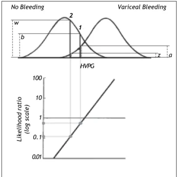
Figure 5. Likelihood ratio based on probability densities (heights) of the two distribution curves for variceal bleeding and no bleeding at the actual HVPG level. For this procedure to be valid both distribution curves should be normal and have the same standard deviation. In example 1 the likeliho-od ratio of bleeding to no bleeding is 0.5 since the height (a)
up to the curve for variceal bleeding is only half the height
(b) up to the curve for no bleeding. In example 2 the likeli-hood ratio of bleeding to non-bleeding is 0.12 since the height
(z) up to the curve for variceal bleeding is only 0.12 of the height (w) up to the curve for non-bleeding. Thus for a given patient the risk of bleeding can be estimated from his/her ac-tual HVPG level.
WEAKNESSES OF DICHOTOMIZATION
The preceding methods of utilizing the informa-tion provided by a quantitative diagnostic variable like HVPG involve dichotomization defining ‘nor-mal’ and ‘abnor‘nor-mal’. Thus the quantitative informa-tion provided by the test-value within each of the two defined groups (normal or abnormal) is not uti-lized. All test-values smaller than the cutoff are con-sidered equal and all test-values larger than the cutoff are also considered equal. By disregarding the actual value of the test-variable within each of the groups (normal, abnormal) information is lost.
STRENGTH OF EVIDENCE BASED ON TEST-VALUE
In the following a method utilizing quantitative test-values as such without dichotomization will be
described. Considering the HVPG there would be a relation between the risk of bleeding and the actual level of HVPG irrespective any defined threshold: the smaller the HVPG, the lesser the risk of bleeding; the larger the HVPG, the greater the risk of blee-ding.
The risk can be expressed as the likelihood ra-tio (the ratio between the probability densities or heights) of the two distribution curves at the actual HVPG level (Figure 5).19 From the likelihood ratio
and the pre-test probability of bleeding the post-test probability of bleeding can be estimated using Ba-yes’ theorem as shown previously in this paper. However, this likelihood ratio method would only be valid if the distribution curves for bleeding and non-bleeding were normal with the same standard de-viation. These requirements may not be entirely fulfilled in practice. If they are not fulfilled it may be possible to perform a normalizing transformation of the variable or to perform analysis after dividing the information of the quantitative variable into a sma-ller number of groups e.g. 3 or 4 groups.
UTILIZING THE COMBINED INFORMATION OF MORE VARIABLES
Besides the key variable HVPG other descriptive variables (e.g. symptoms, signs and liver function tests) may influence the risk of bleeding from vari-ces. By utilizing such additional information, esti-mation of the risk of bleeding in a given patient may be improved. Such predictive models may be develo-ped using multivariate statistical analysis like logis-tic regression or Cox regression analysis.20,21
In the literature there are many examples of uti-lizing the combined diagnostic information of more variables.22,23 Here will just be mentioned one
example by Merkel, et al. who showed that the pre-diction of variceal bleeding could be improved by supplementing the information provided by HVPG with information of the Pugh score, the size of the esophageal varices and whether variceal bleeding had occurred preciously.24 Their multivariate
mo-del had significantly more predictive power than HVPG alone.
CONCLUSION
The methods for evaluation of simple diagnostic tests provided in this paper are important tools for optimal evaluation of patients. They may, however, have limitations for quantitative variables, since the dichotomization, which needs to be made, has
2 1
z w
a b
No Bleeding Variceal Bleeding
Likelihood
ratio
(log
scale)
100
10
1
0.1
0.01
the consequence that quantitative information is being lost. Quantitative variables should be kept as such whenever possible. Prediction of diagnosis and out-come may be markedly improved if more informative variables can be combined using multivariate statis-tical analysis e.g. logistic regression analysis. Prefe-rably dichotomization of quantitative variables should only be used in the last step, when a binary decision (i.e. yes/no in regard to diagnosis or thera-py) has to be made.
REFERENCES
1. Mayer D. Essential evidence based medicine. Cambridge: Cambridge University Press; 2004.
2. Loong TW. Understanding sensitivity and specificity with the right side of the brain. BMJ 2003; 327: 716-9.
3. Altman DG, Bland JM. Diagnostic tests. 1: Sensitivity and specificity. BMJ 1994; 308: 1552.
4. Akobeng AK. Understanding diagnostic tests 1: sensitivi-ty, specificity and predictive values. Acta Paediatr 2007; 96: 338-41.
5. Altman DG, Bland JM. Diagnostic tests 2: Predictive va-lues. BMJ 1994; 309: 102.
6. Akobeng AK. Understanding diagnostic tests 2: likelihood ratios, pre- and post-test probabilities and their use in cli-nical practice. Acta Paediatr 2007; 96: 487-91.
7. Deeks JJ, Altman DG. Diagnostic tests 4: likelihood ratios.
BMJ 2004; 329: 168-9.
8. Halkin A, Reichman J, Schwaber M, Paltiel O, Brezis M. Likelihood ratios: getting diagnostic testing into perspec-tive. QJM 1998; 91: 247-58.
9. Gill CJ, Sabin L, Schmid CH. Why clinicians are natural ba-yesians. BMJ 2005; 330: 1080-3.
10. Fagan TJ. Nomogram for Bayes theorem. N Engl J Med
1975; 293: 257.
11. Altman DG, Bland JM. Diagnostic tests 3: receiver opera-ting characteristic plots. BMJ 1994; 309: 188.
12. Akobeng AK. Understanding diagnostic tests 3: Receiver operating characteristic curves. Acta Paediatr 2007; 96: 644-7.
13. Vining DJ, Gladish GW. Receiver operating characteristic curves: a basic understanding. Radiographics 1992; 12: 1147-54.
14. Lasko TA, Bhagwat JG, Zou KH, Ohno-Machado L. The use of receiver operating characteristic curves in biomedical informatics. J Biomed Inform 2005; 38: 404-15.
15. Kim B, Basso MA. Saccade target selection in the superior colliculus: a signal detection theory approach. J Neurosci
2008; 28: 2991-3007.
16. Tosteson TD, Buonaccorsi JP, Demidenko E, Wells WA. Measurement error and confidence intervals for ROC cur-ves. Biom J 2005; 47: 409-16.
17. Hanley JA, McNeil BJ. A method of comparing the areas un-der receiver operating characteristic curves un-derived from the same cases. Radiology 1983; 148: 839-43. 18. Hajian-Tilaki KO, Hanley JA. Comparison of three methods
for estimating the standard error of the area under the curve in ROC analysis of quantitative data. Acad Radiol
2002; 9: 1278-85.
19. Armitage P, Berry G. Statistical methods in medical resear-ch. 3rd. Ed. Oxford: Blackwell Scientific Publications; 1994.
20. Christensen E. Multivariate survival analysis using Coxs regression model. Hepatology 1987; 7: 1346-58.
21. Christensen E. Prognostic models including the Child-Pugh, MELD and Mayo risk scoreswhere are we and where should we go? J Hepatol 2004; 41: 344-50.
22. Porcel JM, Peña JM, Vicente de Vera C, Esquerda A, Vives M, Light RW. Bayesian analysis using continuous likelihood ratios for identifying pleural exudates. Respir Med 2006; 100: 1960-5.
23. Miettinen OS, Henschke CI, Yankelevitz DF. Evaluation of diagnostic imaging tests: diagnostic probability estima-tion. J Clin Epidemiol 1998; 51: 1293-8.