Received XXXX
(www.interscience.wiley.com) DOI: 10.1002/sim.0000 MOS subject classication: 92D25; 65M25; 65M12; 35B40
A numerical study on the estimation of the
stable size distribution for a cell population
balance model
Luis M. Abia
b
,
Oscar Angulo
a
, Juan Carlos Lopez-Marcos
b
and Miguel
Angel Lopez-Marcos
b
The presence of a steady-state distribution is an important issue in the modelization of cell populations. In this paper, we analyse, from a numerical point of view, the approach to the stable size distribution for a size-structured balance model with an asymmetric division rate. To this end, we introduce a second order numerical method based on the integration along the characteristic curves over the natural grid. We validate the interest of the scheme by means of a detailed analysis of convergence. Copyright c 0000 John Wiley & Sons, Ltd.
Keywords: cell population balance models; asymmetric division; numerical methods; natural grid; convergence analysis; stable size distribution
1. Introduction
We consider the numerical integration of a model which is based on the one proposed by Ramkrishna [19]. It describes the evolution of a size-structured cell population and takes the following form
ut(x; t) + (g(x) u(x; t))x = (x) u(x; t) b(x) u(x; t) + 2
∫ 1
x b(s) P (x; s)u(s; t) ds; xmin< x < 1; t > 0; (1.1)
u (xmin; t) = 0; t > 0; (1.2)
u(x; 0) = '(x); xmin x 1: (1.3)
The independent variables x and t represent size and time respectively, xmin stands for a nonnegative minimum cell-size and we
consider a maximal cell-size, normalized to 1. The dependent variable u(x; t) is the size-specic density of cells with size x at time t. The size of any cell varies according to the following ordinary dierential equation
dx
dt = g(x);
aDepartamento de Matematica Aplicada e IMUVA. ETSIT. Universidad de Valladolid. 47011 Valladolid. SPAIN.
bDepartamento de Matematica Aplicada e IMUVA. Facultad de Ciencias. Universidad de Valladolid. 47011 Valladolid. SPAIN.
where g(x) is the growth rate with g > 0 on [xmin; 1). The nonnegative functions and b represent the mortality and division
rates respectively. These are usually called the vital functions and dene the life history of cells. Finally, the distribution of sizes between the two daughter cells at the moment of cell division (unequal division) is dened in terms of a conditional density P (x; y), called the partitioning function, which gives the distribution of the size of a daughter-cell x, when the size of the mother is equal to y. Thus,
∫ x2
x1
P (x; y) dx means the probability for a daughter cell to have size x in the interval (x1; x2) knowing that
the mother had size y. Such distribution should verify the following properties:
∫1
xmin
P (x; y) dx = 1; P (x; y) = P (y x; y); P (x; y) = 0; x y:
As a particular (and extreme) case, mother cells could always divide into two identical daugther cells (equal division). In that case, the partitioning function reduces to the Dirac delta function P (x; y) = (x y=2), and it turns into the model proposed by Diekmann et al. [8]. In these models, the environment is assumed to have unlimited space and resources.
A remarkable feature is the existence of a maximum individual size. This is a biological truth: cells must divide or die before reaching this value. Therefore, (1) = 0 where
(x) = exp
( ∫ x
xmin
(s) + b(s)
g(s) ds
)
; xmin x 1;
which represents the probability that an individual of size xmin reaches size x. If the division and mortality rates are bounded
functions, cells will not disappear at the maximum size and the previous condition cannot be satised unless they do not reach such a value. For this purpose, we consider a growth function that veries lim
x!1
∫ x xmin
ds
g(s) = +1. Note that this hypothesis implies g(1) = 0 if g is a continuous function dened in [xmin; 1]. Henceforth, in the present model, we assume that cell-size is
strictly increasing during lifetime of cells and always less than one. Moreover, if we assume that initially there are no cells of maximum size, the solution to the problem satises u(1; t) = 0, t > 0 [7].
Cell population balance models were introduced in the early 1960s within the framework of particle dynamics in chemical and cellular contexts [21, 5, 11]. Despite this early development, nowadays it is an area of increasing applications and it is used to describe quite dierent issues (see [20] and references therein). In recent years, they have evolved towards more complicated models: several structuring variables, various populations (describing, for example, proliferating and quiescent cells or the dierent stages in a cell-cycle), nonlinear problems (with the consumption of a limited extracellular medium), inverse problems to compute the vital functions [6, 9, 10, 22]. In our setting, we consider a cell population balance model structured by the cell-size in which the reproduction is carried out by ssion into two daughter cells with dierent sizes. Cell-size is an attractive variable as a result of the relative ease and precision with which it can be measured because the instrumentation to obtain it has improved considerably. The model that arises because of this simplication is still useful in order to analyse and understand cell population dynamics.
From a theoretical point of view, a general survey of the main mathematical problems solved and the principal techniques employed in this context is given in [17, 16, 4, 18]. Properties such as existence, uniqueness, etc., could be studied without an explicit expression for the solution. However, the knowledge of their qualitative or quantitative behaviour in a more tangible way sometimes becomes necessary. Therefore, numerical methods provide a valuable tool to obtain such information.
One of the most important issues in the formulation of cell population balance models from both a qualitative and quantitative point of view is to establish the existence of a size pyramid. The main purpose in the study of system (1.1)-(1.3) has been to set the experimental evidence of a stable size distribution. A size distribution is represented as
u(x; t)
∫1
xminu(x; t) dx
: (1.4)
A stable steady distribution is achieved if there exists a function (x) such that the size distribution tends to (x), as time t tends to +1. The existence of implies a solution of (1.1)-(1.3) of the type C e t(x) where is an asymptotic value of the
may be, it is shaped asymptotically as the function u, this property is called asynchronicity. Even if the initial distribution has a
very narrow support, it will tend to occupy asymptotically the whole support of , therefore we can generate a large population (a clone) from a single cell. From a theoretical point of view, several authors have proved the existence of stable size distribution with dierent hypotheses [8, 13].
From a numerical point of view, in the last twenty years, several studies have addressed their numerical solution with dierent techniques: analytical solutions based on a successive generations approach, classical nite dierence schemes, nite element or spectral methods or the use of the integration along the characteristics (see [2] and references therein). However, the analysis of most of these numerical proposals is not nished yet and its convergence to the theoretical solution has been ensured only in a few of them [3]. In the present paper, we present a second-order characteristics method, based on the numerical scheme developed and analysed in [3] for the symmetric division case. Second-order methods maintain a good compromise between the required smoothness of the vital functions based on realistic biological data and the eciency of the numerical schemes. We employ a numerical approximation to an invariant grid on the state variable and the discretization of the integral representation of the solution to the problem along the characteristic curves. We also prove the optimal rate of convergence under appropriate regularity assumptions.
The paper is organized as follows. In Section 2, we introduce the proposed numerical method. Section 3 is devoted to a representative numerical simulation which shows how we use the new method to approximate the stable size distribution of the model. Finally, we strengthen the rationale for the scheme with an appendix where we analyse the convergence of the numerical solution.
2. Numerical Method
We rewrite (1.1) as
ut(x; t) + g(x) ux(x; t) = (x) u(x; t) + 2
∫ 1
x b(s) P (x; s)u(s; t) ds; xmin< x < 1; t > 0; (2.1)
where we have dened (x) = g0(x) + (x) + b(x). We denote by x(t; t
; x) the characteristic curve of the equation (2.1)
(and (1.1)) that takes the value xat the time instant t, and dene w(t; t; x) = u(x(t; t; x); t), t t. Thus,
d
dtx(t; t; x) = g(x(t; t; x)); t > t; x(t; t; x) = x;
(2.2)
and
d
dtw(t; t; x) = (x(t; t; x)) w(t; t; x) + 2
∫ 1
x(t;t;x)
b(s) P (x(t; t; x); s)u(s; t) ds; t > t;
w(t; t; x) = u(x:t):
(2.3)
We will obtain a numerical approximation to the solution u of (2.1) and (1.2)-(1.3) on a xed time interval [0; T ]. The numerical method comprises two basic steps. The rst one is to build a grid f(xj; tn) : 0 j J + 1; 0 n Ng, on [xmin; 1] [0; T ],
with xmin= x0< x1< < xJ< xJ+1= 1, such that points (xj; tn) and (xj+1; tn+1), 0 j J + 1, 0 n N, belong to the
same characteristic curve. This time-invariant grid is usually known as the natural grid and was rst introduced in [15]. Its invariance allows us to study the long-term behaviour of the model which has proven to be one of the easiest ways to discretise the population states (cell-sizes). With this aim, we solve numerically (2.2) with an integrator for ordinary dierential equations. The second step is to compute an approximation to u(xj+1; tn+1) starting from a numerical approach to u(xj; tn). To this end,
we discretize the solution to (2.3), which is given by
w(t; t; x) = u(x; t) exp
{ ∫ t t
(x(; t; x)) d
}
+ 2
∫t
t exp
{ ∫ t
(x(s; t
; x)) ds
} (∫ 1
x(;tb() P (x(; t;x) ; x); ) u(; )d
)
This approximation technique has been applied to dierent models in [2] and [3]. On the one hand, a useful rst-order scheme was proposed to obtain the solution to a nonlinear generalization of (1.1)-(1.3) when the vital functions involved in the problem depend on an abiotic environment that changes with time [2]. It is known that low-order of convergence would produce a lack of eciency which could be reduced with higher order methods. However, the smoothness of the solution to (1.1)-(1.3) is not as high as these last schemes demand. Thus, second-order methods present a good balance: they enhance the eciency even with a lack of regular data. On the other hand, a novel second-order method was introduced for the equal ssion model in [3]. In this work, we present an adaptation of this method to the more general asymmetric division case.
2.1. The grid points
Let N be a positive integer. We dene k = T
N and introduce the discrete time levels tn= n k, 0 n N. As we have mentioned,
we want to introduce a state variable grid
xmin= x0< x1< < xJ< xJ+1= 1; (2.5)
such that points (xj; tn) and (xj+1; tn+1), 0 j J + 1, 0 n N, belong to the same characteristic curve. This grid is
nonuniform and invariant with time because the growth rate function is, explicitly, independent of the time variable. We want to stress that J is an a posteriori chosen integer and represents the last grid point computed. In general, we are unable to solve (2.2) analytically, hence we integrate it numerically. We consider the grid points dened by the equations
x0= xmin; xj+1= xj+k2 (g(xj) + g(xj + kg(xj))); 0 j J 1; xJ+1= 1; (2.6)
where we employ the modied Euler method, a second order Runge-Kutta method. In [1], it is stated that we need the continuity and positivity of function g on [0; 1) to satisfy (2.5) and ensure the existence of xJ, such that K0k < 1 xJ K1k, with K0
and K1 suitable constants. It also establishes estimates for the local error when g is smooth enough. Note that actually the
points (xj; tn) and (xj+1; tn+1), 0 j J 1, 0 n N 1, belong to the same numerical characteristic curve.
2.2. Numerical integration along the characteristics
We refer to the grid point xj by a subscript j and to the time level tnby a superscript n. Let Ujnbe a numerical approximation to
un
j = u(xj; tn), 0 j J 1, 0 n N 1. The next stage is to propose a one-step method in order to obtain an approximation
Un+1
j+1 to uj+1n+1. To this end, we use, with step size k, the following second-order discretization of (2.4). For 0 n N 1,
Uj+1n+1= exp
{
k
2((xj) + (xj+1))
} (
Unj+ k Qjk(bPjUn)
)
+ k Qj+1k (b Pj+1 Un+1); 0 j J 1: (2.7)
In this formula, Ql
k(V) represents a quadrature rule to approximate the integral over the interval [xl; 1], 0 l J, of the function
with grid values V = [V0; : : : ; VJ+1]. In this case b, Pl and Um, represent the vectors with components [b(x0); : : : ; b(xJ+1)],
[P (xl; x0); : : : ; P (xl; xJ+1)] and [U0m; : : : ; UJ+1m ], respectively, and products b Pl Um, 0 l J, 0 m N, must be interpreted
component-wise. The approximating values at the minimum and maximum sizes are
Un+1
0 = UJ+1n+1= 0: (2.8)
With regard to the nonlocal terms, we consider the composite trapezoidal quadrature rule on the grid inside the interval [xl; 1]
Qlk(V) = J
∑
j=l
xj+1 xj
2 (Vj+ Vj+1) ; l = 0; : : : ; J: (2.9)
The numerical procedure seems to be implicit. However, if we compute the approximations at the new time level tn+1downwards
(that is, rst Un+1
J+1using (2.8), then Uj+1n+1from J 1 to 0 using (2.7), and nally U0n+1using (2.8) again), it results in an explicit
Assuming suitable regularity conditions in the vital functions and the solution to problem (1.1)-(1.3), we can prove the second order convergence of the numerical approximation to the exact solution u. We want to emphasise that the number of nodes in the natural grid is not determined with respect to N (and therefore, with respect to k), but even so we obtain the convergence of the quadrature rule under this premise. In [1], conversely, a subgrid of the natural grid is introduced to overcome this diculty. In Appendix A, we provide the demonstration based on the consistency property of the method. This result has been validated by means of an extensive numerical simulation carried out with dierent text problems, nal-times T and step-sizes k, not included in this paper.
3. Numerical study on the Stable Size distribution
Taking into account the interest of the discretization method in the numerical approximation of problem (1.1)-(1.3), we use it for the analysis of the associated stable size distribution. The model has a stable size distribution if there exists a function (x) and a value such that
(x) = (g(x) (x))0 ((x) + b(x)) (x) + 2∫ 1
x b(s) P (x; s) (s) ds; (xmin) = 0:
And, if we denote
P (t) =
∫ 1
xmin
u(x; t) dx;
the function u(x; t)=P (t) tends to (x), as time t tends to +1. The existence of a distribution (x) implies the existence of a solution of (1.1)-(1.3) of the type e t(x). The number is unique and known as the malthusian parameter of system
(1.1)-(1.3). A remarkable feature is the asynchonicity [4], i.e., it is possible to start from a single cell and generate a large population. The existence of a stable-size distribution for our problem could be studied in two dierent ways following the techniques employed in [13, 12, 14]. Firstly, by means of a change of variable that transforms the problem into an age-structured one. Secondly, with the use of specic division rate functions as, for example, (3.10).
The following simulation shows the appearance of the asynchronous exponential growth with one of the experiments introduced in [2]. We introduce a minimum size a at which a cell divides, xmin a < 1, to incorporate a more realistic behaviour. So, we
assume that the division rate b vanishes at the interval [xmin; a]. We consider xmin= 0, a = 14, (x) = 0, g(x) = 0:1 (1 x). We
use the size-specic division rate function
b(x) =
0; if x 2[0;1 4
]
;
g(x) b(x)
1 ∫1=4x b(s) ds; if x 2
[1
4; 1
]
; (3.10)
where we have considered that each cell has a stochastically predetermined size at which ssion has to occur, which is given by a probability density b [17]. In this case
b(x) =
(
x 1
4
)3; if x 2[1 4;58
]
;
459 4096 94
(
x 13 16
)2
+16(x 13 16
)4
; if x 2[5 8; 1
]
;
and =81920
3159. We take the same partitioning function as in [2],
P (x; y) =
1 (40; 40)
1 y
(
x y
)39(
1 xy
)39
; if x < y;
0; if x y;
(3.11)
Hence, we compute an approximation to the stable size distribution by using the numerical solution obtained with the numerical method. We describe the evolution of the size-distribution with a numerical counterpart of (1.4), that is
Un j
Q0
k(Un); 0 j J + 1;
that will converge to U
j, 0 j J + 1, an approximation of the stable size distribution if it exists. We observe that a good
approximation to the stable size distribution is reached with moderate values of T (we observe that T = 100 is enough). Once we reach such values, assuming Un
j C e tnUj, we estimate by means of the comparison of consecutive time steps (using
the total populations, for instance) and C.
First, we show how the problem reaches the stable size distribution. We have made an extensive numerical experimentation with dierent initial conditions with the same conclusion but we show the results we obtain with a compatible initial condition with some oscillations which could have introduced a dierent behaviour,
'(x) =
0; if x 2[0;1 8
]
;
'1 (x 18
)3(1 x) (sin(m x + ) + 1); if x 2[1 8; 1
]
;
(m is an integer, the higher the larger number of oscillations, and coecient '1is chosen in order to assure that the maximum
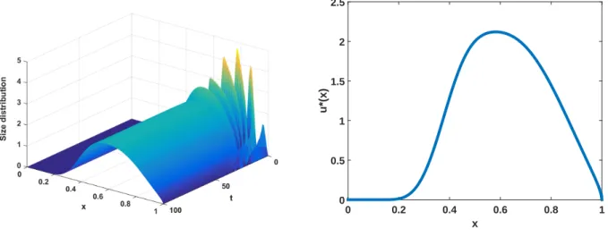
value of '(x) is 1). We have employed dierent values of m but, in Figure 1, we present the simulation with step-size k = 0:01 and m = 20. In the left-hand picture, we show the evolution of the size distribution and, in the right-hand picture, the arising approximation to the stable size distribution. The estimated values of the parameters are = 6:151916e-2 and C = 2:205377.
x
0 0.2 0.4 0.6 0.8 1
u*(x)
0 0.5 1 1.5 2 2.5
Figure 1. Left-hand picture: Evolution of the size distribution. Right-hand picture: Numerical stable size distribution uwith division rate b given in (3.10)
In order to analyse the behaviour of the solution depending on the initial distribution, we have checked with various initial conditions, however here we present only the results obtained with
'(x) =
0; if x 2[0;1 8
]
;
'1(x 18)3(1 x) ; if x 2[18; 1];
(3.12)
( 2 R, coecient '1is chosen in order to assure that the maximum value of '(x) is ). Of course, in all cases, we obtain the
same numerical stable size distribution as presented in Figure 1 (right-hand picture). Table 1 shows the computed values of C and for dierent values of . We clearly observe the independence of the initial data of the Malthusian parameter, while the constant C shows its dependence on it: C is multiplied by the same factor as the initial data.
C 1 4.408119e-1 6.151916e-2 2 8.816239e-1 6.151916e-2 4 1.763248e0 6.151916e-2 8 3.526495e0 6.151916e-2
Table 1. Computed values C and for dierent initial conditions '. T = 100.
data functions will modify it and, likewise, the Malthusian parameter and the constant C. With this purpose, we use again the following data input: xmin= 0, a = 14, (x) = 0, g(x) = 0:1 (1 x), P (x; y) and the initial data as given in (3.11) and (3.12),
= 1, respectively, but now the size-specic division rate is modied as follows,
b(x) = b1
(
x 14
)3
(1 x); 14 x 1; 0; (coecient b
1 is chosen in order to assure that the maximum value of b(x) is 1). As parameter grows, the maximum value
in the division rate is reached at smaller sizes and, then, we expect that the density of larger cells decreases.
The change in the division rate, which we have plotted on the right-hand picture of Figure 2 for dierent values of , implies signicant dierences in the arising steady state (left-hand picture of Figure 2). We observe how the increase of parameter aects its shape. This inuence appears at the locus and value of the maximum of the stable size distribution and, also, at signicant densities in the size variable. When the parameter induces an earlier division, the maximum of the stable size distribution increases and it is obtained at a smaller size (it seems to be at the half value of the corresponding maximum locus in the division rate). Consequently, the domain given by signicant densities decreases.
x
0 0.2 0.4 0.6 0.8 1
u
*(x)
0 0.5 1 1.5 2 2.5 3 3.5 4 4.5 5
γ=0
γ=2 γ=5
x
0 0.2 0.4 0.6 0.8 1
bγ
(x)
0 0.1 0.2 0.3 0.4 0.5 0.6 0.7 0.8 0.9 1
γ=0 γ=2 γ=5
Figure 2. Stable size distribution (left-hand picture) for dierent division rates b(right-hand picture).
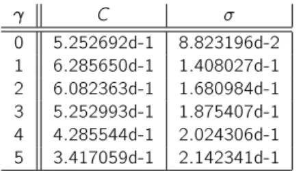
Finally, in Table 2, we display the computed values of and C for dierent values of . We observe, as expected, dierent values of for dierent values of .
4. Conclusions
C 0 5.252692d-1 8.823196d-2 1 6.285650d-1 1.408027d-1 2 6.082363d-1 1.680984d-1 3 5.252993d-1 1.875407d-1 4 4.285544d-1 2.024306d-1 5 3.417059d-1 2.142341d-1
Table 2. Computed values C and for dierent b. T = 100.
adapted to solve this problem and it is dicult to nd theoretical studies that validate them, therefore to design and analyse innovative numerical procedures is really important.
In this study, an important issue in the modelization of cell population balance models has been addressed: the evolution of the size-distribution. We have proposed a suitable scheme to attain the solution of this model which allows us to analyse and approximate the stable size distribution if it exists. We have shown the behaviour of the steady-state distribution in two experiments. The rst one aimed corroborating its independence of the initial size distribution. The second one at exploring its behaviour when the division rate changes. We have observed dierent stable size distributions for each problem and a clear inuence on its maximum, the point at which this maximum is reached and the domain of signicant densities.
The convergence of the numerical method was analysed: second order of convergence under suitable smoothness hypotheses.
A. Convergence Analysis
In this appendix, we carry out the convergence analysis of the scheme introduced in Section 2. From now on, C will denote a positive constant which is independent of k, n (0 n N) and j (0 j J + 1); C possibly has dierent values in dierent places. We denote the maximum norm of v = (v0; v1; : : : ; vJ+1) with jjvjj1.
If u is the solution to problem (1.1)-(1.3), we dene
un= (un
0; un1; : : : ; unJ+1); ujn= u(xj; tn); 0 j J + 1; 0 n N:
The local discretization error, n+1= (n+1
0 ; 1n+1; : : : ; J+1n+1); 0 n N 1, is given by
j+1n+1 = k1
(
un+1j+1 exp
{
k
2 ((xj) + (xj+1))
}(
unj + k Qjk(b Pj un)
)
k Qj+1k (b Pj+1 un+1)
)
; (A.1)
0 j J 1, n+1
0 = J+1n+1= 0.
First of all, note that the magnitude of J is not determined with respect to k. However, we prove the convergence of the composite quadrature rule over such a grid.
Lemma 1 Let f be two times continuously dierentiable, fxjgJ+1j=0 a nonuniform grid satisfying xj+1 xj C k, 0 j J, x0= 0,
xJ+1= 1; and denote with fl= f (xl), 0 l J + 1 the grid values of the function f and with Qlk, 0 l J, the composite
trapezoidal quadrature rules given in (2.9). Then, as k ! 0, the following estimates hold
∫x1
l
f () d Ql
k(f)= O(k2); 0 l J: (A.2)
Proof: From (2.9), we obtain
∫ 1
xl
f () d Ql k(f) =
J
∑
j=l
(∫ xj+1
xj
f () d xj+12 xj (f (xj) + f (xj+1))
)
0 l J. Taking into account the convergence properties of the trapezoidal cuadrature rule,
∫ xj+1
xj
f () d xj+12 xj (f (xj) + f (xj+1)) = (xj+1 xj) 3
12 f00(j); j 2 [xj; xj+1]; (A.4)
we have ∫
1 xl
f () d Qlk(f) = J
∑
j=l
(xj+1 xj)3
12 f00(j); (A.5)
0 l J. Thus
∫x1
l
f () d Ql
k(f) C J
∑
j=l
(xj+1 xj)3 C k2 J
∑
j=l
(xj+1 xj) = C (1 xl) k2: (A.6)
And the estimative (A.2) holds.
Lemma 2 Let g be three times continuously dierentiable, functions , b P and u be two times continuously dierentiable. Then, as k ! 0, the following estimates hold for the local discretization error (A.1)
jjn+1jj
1= O(k2); 0 n N 1: (A.7)
Proof: From (A.1), we obtain
jn+1
j+1j 1kuj+1n+1 u
(
x(tn+1; tn; x
j); tn+1)
+1k u(x(tn+1; tn; x
j); tn+1) k Qj+1k (b Pj+1 un+1) exp
{
k
2 ((xj) + (xj+1))
}(
un
j + k Qjk(b Pj un)
) ; (A.8)
0 j J 1, 0 n N 1. The smoothness of u and g, and the local error estimate for the modied Euler method [1] allow us to conclude
un+1 j+1 u
(
x(tn+1; tn; x
j); tn+1) C k3: (A.9)
In addition, we can use (2.4) to bound the second term on the right-hand side of (A.8) as
u(x(tn+1; tn; xj); tn+1) k Qj+1k (b Pj+1 un+1) exp
{
k
2 ((xj) + (xj+1))
}(
ujn + k Qjk(b Pj un)
) un j exp
{ ∫ tn+1
tn
(x (; tn; x j)) d
}
exp
{
k
2 ((xj) + (xj+1))
}
+2
∫ tn+1
tn exp
{ ∫ tn+1
(x (s; tn; x j)) ds
} (∫ 1
x(;tnb() P (x(; t;xj)
n; x
j); ) u(; ) d
) d k ( exp { k
2((xj) + (xj+1))
}
Qj
k(b Pj un) + Qj+1k (b Pj+1 un+1)
)
: (A.10)
Thus, we use the regularity of functions , b P and g, the convergence properties of the trapezoidal cuadrature rule and the modied Euler method to obtain
exp
{ ∫ tn+1
tn
(x (; tn; x j)) d
}
exp
{
k
2 ((xj) + (xj+1))
}
exp
{ ∫ tn+1
tn
(x (; tn; x j)) d
} exp { k 2 ( (x
j) + (x(tn+1; tn; xj)))}
+ exp { k 2(xj)
} exp { k 2 (
x(tn+1; tn; x
j))} exp
{
k
2(xj+1)
}
C (k3+ k j(x(tn+1; tn; x
With respect to the second term on the right-hand side of (A.10),
2
∫ tn+1
tn exp
{ ∫ tn+1
(x (s; tn; x j)) ds
} (∫ 1
x(;tn;xb() P (x(; tj)
n; x
j); ) u(; ) d
) d k ( exp { k
2((xj) + (xj+1))
}
Qj
k(bPjun)+Qj+1k (bPj+1un+1)
)
2
∫tn+1
tn exp
{ ∫ tn+1
(x (s; tn; x j)) ds
} (∫ 1
x(;tn;xb() P (x(; tj)
n; x
j); ) u(; ) d
) d k 2 ( exp
{ ∫ tn+1
tn
(x (s; tn; x j)) ds
} (∫ 1
xj
b() P (xj; ) u(; tn) d
)
+
∫1
x(tn+1;tn;xj)b() P (x(t
n+1; tn; x
j); ) u(; tn+1) d
)
+ kexp
{ ∫ tn+1
tn
(x (s; tn; x j)) ds
} (∫ 1
xj
b() P (xj; ) u(; tn) d
)
exp
{
k
2 ((xj) + (xj+1))
}
Qjk(b Pj un)
+ k
∫ 1
x(tn+1;tn;xb() P (x(tj)
n+1; tn; x
j); ) u(; tn+1) d Qj+1k (b Pj un+1)
: (A.12)
The rst term on the right-hand side of (A.12) is O(k3) as a result of the properties of the local error for the trapezoidal
quadrature rule. With respect to the second term on the right-hand side of (A.12), we have
exp
{ ∫ tn+1
tn
(x (s; tn; x j)) ds
} (∫ 1 xj
b() P (xj; ) u(; tn) d
)
exp
{
k
2 ((xj) + (xj+1))
}
Qj
k(b Pj un)
exp
{ ∫ tn+1
tn
(x (s; tn; x j)) ds
}
exp
{
k
2 ((xj) + (xj+1))
} ∫ 1 xj
b() P (xj; ) u(; t) d
+ exp { k
2 ((xj) + (xj+1))
}
∫ 1
xj
b() P (xj; ) u(; tn) d Qjk(b Pj un)
:
Note that the numerical grid is computed by the modied Euler method and then satises the hypotheses of Lemma 1 [1]. Thus, taking into account the assumed regularity of the vital functions and solution, the second order convergence of the composite quadrature rule (Lemma 1) and (A.11), we conclude that the previous term is O(k2).
Finally, the third term on the right-hand side of (A.12) is bounded as follows
∫ 1
x(tn+1;tn;xb() P (x(tj)
n+1; tn; x
j); ) u(; tn+1) d Qj+1k (b Pj un+1)
∫ xj+1
x(tn+1;tn;xj)b() P (x(t
n+1; tn; x
j); ) u(; tn+1) d
+ ∫1 xj+1
b()(P (x(tn+1; tn; x
j); ) P (xj+1; ))u(; tn+1) d
+ ∫ 1 xj+1
b() P (xj+1; ) u(; tn+1) d Qj+1k (b Pj+1 un+1)
:
And, we can conclude, as previously, that this term is O(k2).
Thus, we establish for the left term on (A.12)
2
∫ tn+1
tn exp
{ ∫ tn+1
(x (s; tn; x j)) ds
} (∫ 1
x(;tnb() P (x(; t;xj)
n; x
j); ) u(; ) d
) d k ( exp { k
2((xj) + (xj+1))
}
Qj
k(b Pj un)+ Qj+1k (b Pj+1un+1)
)
and from (A.11), we observe that the right-hand side of (A.10) is O(k3). The substitution of this bound and (A.9) in (A.8)
produces the estimate (A.7).
Now, we prove the convergence of the numerical method. We denote the error produced by the numerical approximation as
En= (En
0; : : : ; EJn; EJ+1n ); Ejn= ujn Ujn; 0 j J + 1;
0 n N. Note that un
j are the nodal values of the theoretical solution and Ujn are the numerical approximations obtained by
means of the numerical method.
Theorem 3 Assuming the hypotheses of Lemma 2, if kE0k
1= O(k2), as k ! 0, then
kEnk
1= O(k2); 0 n N;
as k ! 0.
Proof: From equations (A.1) and (2.7), we have
Ej+1n+1 = exp
{
k
2 ((xj) + (xj+1))
} (
Ejn+ k Qjk(b Pj En)
)
+ k Qj+1k (b Pj+1 En+1) + k j+1n+1;
0 j J 1, 0 n N 1.
Therefore, taking into account the smoothness properties of the functions and b we arrive at,
jEn+1
j+1j (1 + C k) jEjnj + C k
(
kEnk
1+ kEn+1k1)+ k jj+1n+1j;
0 j J 1, 0 n N 1, and then
kEn+1k
1 (1 + C k) kEnk1+ C k kEn+1k1+ k kn+1k1:
0 n N 1. By means of the discrete Gronwall's lemma, we arrive at
kEnk1 C
{
kE0k1+ n
∑
l=1
k klk1
}
;
1 n N. Now, the estimative holds from (A.7).
Acknowledgements
This work was supported in part by projects MTM2014-56022-C2-2-P and MTM2017-85476-C2-1-P:of the Spanish Ministerio de Economa y Competitividad and European FEDER Funds, and by project VA041P17 of the Junta de Castilla y Leon and European FEDER Funds.
References
1. Angulo O, Lopez-Marcos JC. Numerical schemes for size-structured population equations. Mathematical Biosciences 1999; 157: 169{188.
2. Angulo O, Lopez-Marcos JC, Lopez-Marcos MA. A semi-Lagrangian method for a cell population model in a dynamical environment. Mathematical and Computer Modelling 2013; 57: 1860{1866.
4. Arino O. A survey of structured cell population dynamics. Acta Biotheoretica 1995; 43: 3{25.
5. Bell GI, Anderson EC. Cell growth and division: I. a mathematical model with applications to cell volume distributions in mammalian suspension cultures. Biophysical Journal 1967; 7: 329{351.
6. Borges R, Calsina A, Cuadrado S. Oscillations in a molecular structured cell population model. Nonlinear Analysis: Real Word Applications 2011; 12: 1911{1922.
7. Cushing JM. An Introduction to Structured Population Dynamics. CMB-NSF Regional Conference Series in Applied Mathematics 71, SIAM: Philadelphia; 1998.
8. Diekmann O, Heijmans HJAM, Thieme HR. On the stability of the cell size distribution. Journal of Mathematical Biology 1984; 19: 227{248.
9. Fadda S, Cincotti A, Cao G. A Novel Population Balance Model to Investigate the Kinetics of In Vitro Cell Proliferation: Part I. Model Development. Biotechnology and Bioengineering 2012; 109: 772{781.
10. Fadda S, Cincotti A, Cao G. A Novel Population Balance Model to Investigate the Kinetics of In Vitro Cell Proliferation: Part II. Numerical Solution, Parameters, Determination, and Model Outcomes. Biotechnology and Bioengineering 2012; 109: 782{796. 11. Fredrickson AG, Ramkrishna D, Tsuchiya HM. Statistics and dynamics of procaryotic cell populations. Mathematical Biosciences 1967;
1: 327{374.
12. Gyllenberg M, Webb GF. Asynchronous Exponential Growth of Semigroups of Nonlinear Operators, J. Math. Anal. Appl. 1992; 167: 443-467.
13. Heijmans HJAM. On the stable size distribution of populations reproducing by ssion into two unequal parts. Mathematical Biosciences 1984; 72: 19-50.
14. Kato N. A general model of size-dependent population dynamics with nonlinear growth rate. J. Math. Anal. Appl. 2004; 297: 234-256. 15. Ito K, Kappel F, Peichl G. A fully discretized approximation scheme for size-structured population models. SIAM Journal of Numerical
Analysis 1991; 28: 923{954.
16. Lasota A, Mackey MC. Probabilistic Properties of Deterministic Systems. Cambridge University Press: London; 1985.
17. Metz JAJ, Diekmann O (Eds.). The Dynamics of Physiologically Structured Populations. In: Lect. Notes Biomath. 68, Springer-Verlag: New York; 1986.
18. Perthame B. Transport Equations in Biology. Birkhuser: Basel, Switzerland; 2007.
19. Ramkrishna D. Statistical models of cell populations. In: Advances in Biochemical Engineering. 11, Springer: Berlin; 1979; 1{47, . 20. Ramkrishna D, Singh MR. Population Balance Modeling: Current Status and Future Prospects. Annual Review of Chemical and
Biomolecular Engineering. 2014; 5: 123-146.
21. Randolph AD. A population balance for countable entities. The Canadian Journal of Chemical Engineering. 1964; 42: 280{281. 22. Spetsieris K, Zygourakis K. Single-Cell Behavior and Population Heterogeneity: Solving an Inverse Problem to Compute the Intrinsic