A second order numerical method for a cell population model with asymmetric division

Q1

Contents lists available atScienceDirect

Journal of Computational and Applied

Mathematics

journal homepage:www.elsevier.com/locate/cam

A second-order numerical method for a cell population

model with asymmetric division

Q2 ∧

O.

∧

Angulo

a,∗

,

∧

J.C.

∧

López-Marcos

b

,

∧

M.A.

∧

López-Marcos

b

a_{Departamento de Matemática Aplicada e IMUVA, ETSIT, Universidad de Valladolid, Pso. Belén 5, 47011 Valladolid, Spain}

b_{Departamento de Matemática Aplicada e IMUVA, Facultad de Ciencias, Universidad de Valladolid, Pso. Belén 7, 47011 Valladolid, Spain}

a r t i c l e i n f o

Article history:

Received 26 October 2015

Received in revised form 1 February 2016

MSC:

92D25 92D40 65M25 65M12 35B40

Keywords:

Size-structured population Cell population models Asymmetric division Numerical methods Characteristics method Convergence analysis

a b s t r a c t

Population balance models represent an accurate and general way of describing the compli-cated dynamics of cell growth. In this paper we study the numerical integration of a model for the evolution of a size-structured cell population with asymmetric division. We present and analyze a novel and efficient second-order numerical method based on the integration along the characteristic curves. We prove the optimal rate of convergence of the scheme and we ratify it by numerical simulation. Finally, we show that the numerical scheme serves as a valuable tool in order to approximate the stable size distribution of the model.

©2016 Published by Elsevier B.V.

1. Introduction

1

In the framework of the continuum modeling of cell kinetics, cell population balance models have become the most

2

important theoretical tool for describing the proliferation of cells taking place in a cell culture. These ones can be included

3

in the so-called structured population models which describe the evolution of a population by means of the vital properties

4

of individuals (growth, fertility, mortality, division, etc.). Such intrinsic physiological state rates depend on individual

5

characteristics (such as age or size) which structure the population. Cell population balance models were considered for the

6

first time in the sixties (see, for example, [1,2]) and were developed rapidly [3–5]. In recent years, they have evolved towards

7

more complicated models: several structuring variables, various populations (describing, for example, proliferating and

8

quiescent cells or the different stages in a cell-cycle), nonlinear problems (with the consumption of a limited extracellular

9

medium), inverse problems to compute the vital functions [6–9].

10

When reproduction occurs by fission it seems appropriate to take into account the size of individuals (by which we mean

11

any relevant quantity, like mass, volume, weight, protein or DNA content, etc.). In this work, we suppose that cells are only

12

distinguished in terms of this physiological characteristic. The model that arises due to this simplification is still useful in

13

order to analyze and understand the cell population dynamics. Cell size varies over time, and maturation can be simulated

14

∗_{Corresponding author. Tel.: +34 983 423000(Ext: 5835); fax: +34 983 423661.}

E-mail addresses:[email protected](O. Angulo),[email protected](J.C. López-Marcos),[email protected](M.A. López-Marcos).

http://dx.doi.org/10.1016/j.cam.2016.03.008

assuming its increase with the cell-life cycle. To be precise, we consider the cell population balance model proposed by 1

Ramkrishna [10] which considers reproduction by fission into two daughter cells with different size. 2

Theoretical properties of the models such as existence, uniqueness, smoothness of solutions, long-time behavior (with 3

the study of steady states and their stability) could be studied without a solution expression. However, the knowledge of 4

their qualitative or quantitative behavior in a more tangible way is sometimes necessary. Therefore, numerical methods 5

provide a valuable tool to obtain such information. In the case of general structured population models, many numerical 6

methods have been proposed to solve them (see [11,12] and references therein). In the case of cell population balance 7

models different techniques have been used (see [13] and the references therein). However, it is very important to design 8

numerical schemes specially adapted to the characteristics of cell population balance models. 9

Moreover, one of the most important issues in the modelization is whether or not a stable size distribution exists, 10

and many efforts were directed towards describing the most general models which still exhibit a stable type distribution 11

property [14]. 12

In this work we present a second-order characteristics method, based on the numerical scheme developed and analyzed 13

in [13] for the symmetric division case. It is based on the discretization of the integral representation of the solution to 14

the problem along the characteristic curves. Second-order methods maintain a good compromise between the required 15

smoothness of the vital functions based on realistic biological data and the efficiency of the numerical schemes. 16

In Section2we introduce the model and Section3is devoted to the description of the proposed numerical method. In 17

Section4we analyze the convergence of the numerical scheme, and in Section5we carry out a representative numerical 18

simulation, including the approximation of the stable size distribution of the model. 19

2. The model 20

We consider a nonnegative minimum cell-sizexminand a maximal size, normalized to 1, at which point every cell might 21

divide or die, so 0

≤

xmin

<

1. We also assume that the environment is unlimited and all possible nonlinear mechanisms 22

are ignored. 23

The problem is given by a conservation law 24

u_t

(

x

,

t

)

+

(

g

(

x

)

u

(

x

,

t

))

_x

= −

µ(

x

)

u

(

x

,

t

)

−

b

(

x

)

u

(

x

,

t

)

+

2



1

x

b

(

s

)

P

(

x

,

s

)

u

(

s

,

t

)

ds

,

25

xmin

<

x

<

1

,

t

>

0

,

(2.1) 26

a boundary condition 27

u

(

xmin

,

t

)

=

0

,

t

>

0

,

(2.2) 28

and an initial size distribution 29

u

(

x

,

0

)

=

ϕ(

x

),

xmin

≤

x

≤

1

.

(2.3) 30

The independent variablesxandtrepresent size and time, respectively. The dependent variableu

(

x

,

t

)

is the size-specific 31

density of cells with sizexat timet. The size of any individual varies according to the following ordinary differential equation 32

dx

dt

=

g

(

x

).

33

The nonnegative functionsg,

µ

andbrepresent the growth, mortality and division rate, respectively. These are usually called 34

the vital functions and define the life history of the individuals. Note that all of them only depend on the sizex(the internal 35

structuring variable). In this case, we also assume thatg

(

x

) >

0 forx

<

1. 36

The dispersion of sizes at division amongst the two daughter cells (unequal division) is defined in terms of the partitioning 37

functionP

(

x

,

y

)

, a probability density function which gives the distribution of the size of a daughter-cellxwhen the size 38

of the mother is equal toy. Thus



x2

x1 P

(

x

,

y

)

dxgives the probability for a daughter cell to have size in the interval

(

x1

,

x2

)

39 knowing that the mother had the sizey. Such a distribution verifies the following conditions: 40



1

xmin

P

(

x

,

y

)

dx

=

1

,

P

(

x

,

y

)

=

P

(

y

−

x

,

y

),

P

(

x

,

y

)

=

0

,

x

≥

y

.

41

In an extreme case, if two daughter cells from a mother cell are always identical (equal fission), the partitioning function 42

reduces to the Dirac delta functionP

(

x

,

y

)

=

δ(

x

−

y

/

2

)

, leading to the model proposed by Diekmann et al. [15]. 43

In accordance with the accepted biological point of view, there exists a maximum size. This means that cells will divide or 44

die with probability one before reaching it. To this end, if

µ

andbare positive and bounded functions, we consider a growth 45

function, introduced by Von Bertalanffy, satisfying limx→1



x xmin

ds

g(s)

= +∞

. Note that ifgis a continuous function defined 46 in [xmin

,

1] then this hypothesis implies thatg

(

1

)

=

0. Thus, the solution to the problem will satisfyu

(

1

,

t

)

=

0,t

>

0, so 47

3. Numerical method

1

In [17], a useful first-order scheme was proposed to obtain the solution to a generalization of(2.1)–(2.3)when the vital

2

functions involved in the problem depend on an abiotic environment that changes with time. The method proposed in that

3

work was based on the discretization of the ordinary differential equations that satisfies the solution along the characteristic

4

curves. It is known that a low-order of convergence would produce a lack of efficiency which could be reduced with higher

5

order methods. However, the smoothness of the solution to(2.1)–(2.3)is not as high as these last schemes demand. Thus,

6

second-order methods present a good balance: they enhance the efficiency even with a lack of regular data.

7

In [13], we developed a novel second-order characteristics method based on the discretization of the integral

8

representation of the solution to the problem along the characteristic curves for the equal fission model. Here we present

9

an adaptation of this method to the more general asymmetric division case.

10

Therefore, we define

µ

∗

(

x

)

=

g′

(

x

)

+

µ(

x

)

+

b

(

x

)

and denote byx

(

t

;

t∗

,

x∗

)

the characteristic curve of ∧

Eq.(2.1)which

11

takes the valuex∗at the time instantt∗. It is the solution to the initial value problem

12







d

dtx

(

t

;

t∗

,

x∗

)

=

g

(

x

(

t

;

t∗

,

x∗

)),

t

>

t∗

,

x

(

t∗

;

t∗

,

x∗

)

=

x∗

.

(3.1)

13

In this way, the solution to(2.1)along a characteristic curve is given by

14

u

(

x

(

t

;

t∗

,

x∗

),

t

)

=

u

(

x∗

,

t∗

)

exp



−



t

t∗

µ

∗

₍

x

(τ

;

t∗

,

x∗

))

d

τ



15

+

2



t

t∗



exp



−



t

τ

µ

∗

₍

x

(

s

;

t∗

,

x∗

))

ds

 

1

x(τ;t∗,x∗)

b

(σ)

P

(

x

(τ

;

t∗

,

x∗

), σ)

u

(σ , τ)

d

σ



d

τ,

t

≥

t∗

.

(3.2)

16

Note that, in this new layout, we have to solve two types of problems: the integration of the equation which defines

17

the characteristic curves (3.1)and the solution to Eqs. (3.2)which provides the solution to the problem along those

18

characteristics. We use discretization procedures in order to solve them.

19

We consider the numerical integration of model(2.1)–(2.3)along the time interval

[

0

,

T

]

. Thus, given a positive integer

20

N, we definek

=

T

Nand introduce the discrete time levelst

n

₌

_{n k, 0}

_≤

_n

_≤

_{N. We begin with the integration of(3.1)which}

21

provides the grid of the method on the cell-size variable. This grid is nonuniform and invariant with time because the growth

22

rate function is, explicitly, independent of the time variable. However, note that it depends on time implicitly conditioned

23

on cell size. It is usually called thenatural grid[11]. In this work, we approximate such a grid by using a second-order scheme

24

for the numerical integration of(3.1): the modified Euler method providing

25

x0

=

xmin

,

xj+1

=

xj

+

k 2



g

(

xj

)

+

g

(

xj

+

kg

(

xj

))



,

0

≤

j

≤

J

−

1

.

(3.3)

26

IntegerJrepresents the index of the last grid point computed at the size interval and is chosen in order to satisfy the condition

27

K0k

<

1

−

xJ

≤

K1k, withK0andK1suitable constants (we refer to [11] for further details). Note that the points

(

xj

,

tn

)

and

28

(

xj+1

,

tn+1

)

, 0

≤

j

≤

J

−

1, 0

≤

n

≤

N

−

1, belong to the same numerical characteristic curve. Finally, we fix the last grid

29

pointxJ+1

=

1.

30

Then, denotingun_j

=

u

(

xj

,

tn

)

, 0

≤

j

≤

J

+

1, 0

≤

n

≤

N, letUjnbe a numerical approximation tou n

j. We propose a

31

one-step method in order to obtain it. Therefore, starting from an approximation to the initial data(2.3)of the problem, for

32

example, the grid restriction of the function

ϕ

, the numerical solution at a new time level is described in terms of the previous

33

one. Such a general step is obtained by means of the following second-order discretization of(3.2). For 0

≤

n

≤

N

−

1,

34

U_jn₊+₁1

=

exp



−

k 2



µ

∗



xj



+

µ

∗



xj+1







U_jn

+

kQj_k

(

b

·

Pj

·

Un

)



+

kQj_k+1

(

b

·

Pj+1

·

Un+1

),

0

≤

j

≤

J

−

1

.

(3.4)

35

In the previous expression,Q_kl

(

V

)

represents a quadrature rule to approximate the integral over the interval

[

xl

,

1

]

, 0

≤

l

≤

J

36

of the function with grid valuesV

= [

V0

, . . . ,

VJ+1

]

. In this caseb,Pl andUm, represent the vectors with components

37

[

b

(

x0

), . . . ,

b

(

xJ+1

)

]

,

[

P

(

xl

,

x0

), . . . ,

P

(

xl

,

xJ+1

)

]

and

[

U0m

, . . . ,

U m

J+1

]

, respectively, and productsb

·

P

l

_·

_Um_{, 0}

_≤

_l

_≤

_J,

38

0

≤

m

≤

N must be interpreted component-wise. Here, a second order quadrature formula is appropriate. However,

39

it should be noted that the magnitude ofJis not determined with respect tok. So, in order to decrease the computational

40

effort, it is useful to consider a quadrature rule over a suitable subgrid

{

xjm

}

M+1

m=0, of the grid defined by(3.3), withM

=

O

(

k

−1

₎

41

nodes. To this end, we construct a subgrid

{

xjm

}

M+1

m=0such thatxj0

=

0,xjM+1

=

1, and

42

C0k

≤

xjl+1

−

xjl

≤

C1k

,

0

≤

l

≤

M

,

whereC0andC1are positive constants irrespective ofk(for more details we refer to [11]). Finally, for this problem, we 1

propose the following composite trapezoidal quadrature rule on the previous subgrid, modified in the first subinterval by 2

means of the rectangle formula 3

Ql_k

(

V

)

=

(

xj_ml

−

xl

)

Vj_ml

+

M



m=ml

xjm+1

−

xjm

2



Vjm

+

Vjm+1



,

(3.5) 4

wherexj_ml is the first node of the subgrid satisfyingxjm

≥

xl. 5

Obviously, the approximating values at the minimum and maximum sizes are 6

U₀n+1

=

U_Jn₊+₁1

=

0

.

(3.6) 7

The numerical procedure seems to be implicit. However, if we compute the approximations at the new time leveltn+1 ₈ downwards (that is, firstU_Jn₊+₁1using(3.6), thenU_jn₊+₁1fromJ

−

1 to 0 using(3.4), and finallyU₀n+1using(3.6)again), it results 9

in an explicit procedure. The reason is that the right hand side values in(3.4)corresponding to the timetn+1_{are either zero 10}

or previously computed. 11

4. Convergence analysis 12

In this section, we carry out the convergence analysis of the scheme. It is based on the property of consistency of the 13

method. 14

Ifuis the solution to problem(2.1)–(2.3), we define 15

un

=

(

un₀

,

un₁

, . . . ,

un_J+1

),

un_j

=

u

(

xj

,

tn

),

0

≤

j

≤

J

+

1

,

0

≤

n

≤

N

.

16

Thelocal discretization error,

τ

n+1

₌

_(τ

n+1 0

, τ

n+1 1

, . . . , τ

n+1

J+1

),

0

≤

n

≤

N

−

1 is given by 17

τ

n+1 j+1

=

1 k



un_j++₁1

−

exp



−

k 2



µ

∗



xj



+

µ

∗



xj+1







un_j

+

kQj_k

(

b

·

Pj

·

un

)



−

kQj_k+1

(

b

·

Pj+1

·

un+1

)



,

18

0

≤

j

≤

J

−

1

,

(4.1) 19

20

τ

n+1 0

=

τ

n+1

J+1

=

0

.

21

For a vectorv

=

(v

₀

, v

₁

, . . . , v

_J+1

)

, we denote by

∥

v

∥

∞its maximum norm. 22

From now on,Cwill denote a positive constant which is independent ofk,n(0

≤

n

≤

N) andj(0

≤

j

≤

J

+

1);Cpossibly 23

has different values in different places. 24

Lemma 1. Let g be three times continuously differentiable, functions

µ

, b

·

P and u be two times continuously differentiable. Then, 25

as k

→

0, the following estimates hold 26

∥

τ

n+1

∥

∞

=

O

(

k2

),

0

≤

n

≤

N

−

1

.

(4.2) 27

Proof. From(4.1), we obtain 28

|

τ

_jn₊+₁1

| ≤

1

k





un_j++₁1

−

u



x



tn+1

;

tn

,

xj



,

tn+1





+

1 k







u



x



tn+1

;

tn

,

xj



,

tn+1



−

kQj_k+1

(

b

·

Pj+1

·

un+1

)

29

−

exp



−

k 2



µ

∗



xj



+

µ

∗



xj+1







un_j

+

kQj_k

(

b

·

Pj

·

un

)











,

(4.3) 30

0

≤

j

≤

J

−

1, 0

≤

n

≤

N

−

1. 31

With respect to the first term on the right-hand side of(4.3), assuming the smoothness ofuandgand taking into account 32

that the numerical grid is computed by the modified Euler method, we conclude that 33





un

+1 j+1

−

u



x



tn+1

;

tn

,

xj



,

tn+1





≤

C k3

.

(4.4) 34

On the other hand, if we observe the second term on the right-hand side of(4.3), the formula(3.2)allows us to write 35









u



x



tn+1

;

tn

,

xj



,

tn+1



−

kQkj+1

(

b

·

Pj

+1

_·

_un+1

₎

₋

_exp



−

k 2



µ

∗



xj



+

µ

∗



xj+1







un_j

+

kQjk

(

b

·

Pj

·

un

)





_





36

≤





un_j















exp



−



tn+1

tn

µ

∗



x



τ

;

tn

,

xj



d

τ



−

exp



−

k 2



µ

∗



xj



+

µ

∗



xj+1















+











2



tn+1

tn

exp



−



tn+1

τ

µ

∗



x



s

;

tn

,

xj



ds

 



1

x(τ;tn_,x j)

b

(σ )

P

(

x

(τ

;

tn

,

xj

), σ)

u

(σ , τ)

d

σ



d

τ

1

−

k



exp



−

k 2



µ

∗



xj



+

µ

∗



xj+1





Q_kj

(

b

·

Pj

·

un

)

+

Q_kj+1

(

b

·

Pj+1

·

un+1

)









.

(4.5) 2

Thus, we use the regularity of functions

µ

,b

·

Pandg, the convergence properties of the trapezoidal ∧

quadraturerule and

3

the modified Euler method to obtain

4











exp



−



tn+1

tn

µ

∗



x



τ

;

tn

,

xj



d

τ



−

exp



−

k 2



µ

∗



xj



+

µ

∗



xj+1







_







5

≤











exp



−



tn+1

tn

µ

∗



x



τ

;

tn

,

xj



d

τ



−

exp



−

k 2



µ

∗



xj



+

µ

∗



x



tn+1

;

tn

,

xj







_







6

+

exp



−

k 2

µ

∗



xj



 







exp



−

k 2

µ

∗



x



tn+1

;

tn

,

xj





−

exp



−

k 2

µ

∗



xj+1











7

≤

C



k3

+

k

|

µ

∗



x



tn+1

;

tn

,

xj



−

µ

∗



xj+1



|



8

≤

C k3

.

(4.6)

9

Next, we bound the second part on the right-hand side of(4.5)as

10











2



tn+1

tn

exp



−



tn+1

τ

µ

∗



x



s

;

tn

,

xj



ds

 



1

x(τ;tn_,x j)

b

(σ)

P

(

x

(τ

;

tn

,

xj

), σ )

u

(σ , τ)

d

σ



d

τ

11

−

k



exp



−

k 2



µ

∗



xj



+

µ

∗



xj+1





Q_kj

(

b

·

Pj

·

un

)

+

Q_kj+1

(

b

·

Pj+1

·

un+1

)









12

≤

2













tn+1

tn

exp



−



tn+1

τ

µ

∗



x



s

;

tn

,

xj



ds

 



1

x(τ;tn_,x j)

b

(σ)

P

(

x

(τ

;

tn

,

xj

), σ )

u

(σ , τ)

d

σ



d

τ

13

−

k 2



exp



−



tn+1

tn

µ

∗



x



s

;

tn

,

xj



ds

 



1

xj

b

(σ )

P

(

xj

, σ)

u

(σ,

tn

)

d

σ



14

+



1

x(tn+1_;tn_,x j)

b

(σ )

P

(

x

(

tn+1

;

tn

,

xj

), σ)

u

(σ ,

tn+1

)

d

σ











15

+

k











exp



−



tn+1

tn

µ

∗



x



s

;

tn

,

xj



ds

 



1

xj

b

(σ)

P

(

xj

, σ )

u

(σ ,

tn

)

d

σ



16

−

exp



−

k 2



µ

∗



xj



+

µ

∗



xj+1





Qj_k

(

b

·

Pj

·

un

)









17

+

k













1

x(tn+1_;tn_,x j)

b

(σ)

P

(

x

(

tn+1

;

tn

,

xj

), σ )

u

(σ,

tn +1

₎

d

σ

−

_Qj_k+1

(

b

·

Pj

·

un+1

)











.

(4.7) 18

The use of the trapezoidal quadrature rule results in the first term on the right-hand side of(4.7)beingO

(

k3

₎

_{. With respect}

19

to the second term on the right-hand side of(4.7), we have

20











exp



−



tn+1

tn

µ

∗



x



s

;

tn

,

xj



ds

 



1

xj

b

(σ )

P

(

xj

, σ )

u

(σ,

tn

)

d

σ



21

−

exp



−

k 2



µ

∗



xj



+

µ

∗



xj+1





Qjk

(

b

·

Pj

·

un

)









22

≤











exp



−



tn+1

tn

µ

∗



x



s

;

tn

,

xj



ds



−

exp



−

k 2



µ

∗



xj



+

µ

∗



xj+1



























1 xj

b

(σ )

P

(

xj

, σ )

u

(σ,

tn

)

d

σ











23

+

exp



−

k 2



µ

∗



xj



+

µ

∗



xj+1

















1 xj

b

(σ)

P

(

xj

, σ )

u

(σ ,

tn

)

d

σ

−

Qjk

(

b

·

P j

_·

_un

₎

Thus, taking into account the assumed regularity of the vital functions and solution, the second order convergence of the 1

composite quadrature rule(3.5), and(4.6), we conclude that the previous term isO

(

k2

)

. 2

Finally, we bound the third term on the right-hand side of(4.7)as follows 3













1

x(tn+1_;tn_,x j)

b

(σ)

P

(

x

(

tn+1

;

tn

,

xj

), σ )

u

(σ,

tn+1

)

d

σ

−

Qj +1 k

(

b

·

P

j

_·

_un+1

₎











4

≤













xj+1

x(tn+1_;tn_,x j)

b

(σ )

P

(

x

(

tn+1

;

tn

,

xj

), σ)

u

(σ ,

tn+1

)

d

σ











5

+













1

xj+1

b

(σ)



P

(

x

(

tn+1

;

tn

,

xj

), σ )

−

P

(

xj+1

, σ )



u

(σ,

tn+1

)

d

σ











6

+













1

xj+1

b

(σ)

P

(

xj+1

, σ )

u

(σ,

tn+1

)

d

σ

−

Qj

+1 k

(

b

·

P

j+1

_·

_un+1

₎











.

7

And, we can conclude, as previously shown, that this term isO

(

k2

₎

_{. 8}

Thus, we can settle for the left term on(4.7) 9











2



tn+1

tn

exp



−



tn+1

τ

µ

∗



x



s

;

tn

,

xj



ds

 



1

x(τ;tn_,x j)

b

(σ )

P

(

x

(τ

;

tn

,

xj

), σ )

u

(σ , τ)

d

σ



d

τ

10

−

k



exp



−

k 2



µ

∗



xj



+

µ

∗



xj+1





Q_kj

(

b

·

Pj

·

un

)

+

Q_kj+1

(

b

·

Pj+1

·

un+1

)









11

≤

C k3

,

(4.8) 12

and from(4.6), we observe that the right-hand side of(4.5)isO

(

k3

)

. The substitution of this bound and(4.4)in(4.3)produces 13

the estimate(4.2). 14

In the following result, we prove the convergence of the numerical method. We denote the error produced by the 15

numerical approximation as 16

En

=

(

E₀n

, . . . ,

E_Jn

,

E_Jn+1

),

Ejn

=

unj

−

Ujn

,

0

≤

j

≤

J

+

1

,

17

0

≤

n

≤

N, (remember thatun_j are the nodal values of the theoretical solution andU_jnare the numerical approximations 18

obtained by means of the numerical method). 19

Theorem 2. Under the hypotheses of Lemma1, if

∥

E0

∥

∞

=

O

(

k2

)

, as k

→

0, then 20

∥

En

∥

∞

=

O

(

k2

),

0

≤

n

≤

N

,

21

as k

→

0. 22

Proof. From Eqs.(4.1)and(3.4), we have 23

E_jn₊+₁1

=

exp



−

k 2



µ

∗



xj



+

µ

∗



xj+1







E_jn

+

kQj_k

(

b

·

Pj

·

En

)



+

kQj_k+1

(

b

·

Pj+1

·

En+1

)

+

k

τ

_jn₊+₁1

,

24

0

≤

j

≤

J

−

1, 0

≤

n

≤

N

−

1. 25

Then, taking into account the smoothness properties of the functions

µ

∗_{andbwe arrive at,}

26

|

E_jn₊+₁1

| ≤

(

1

+

C k

)

|

E_jn

| +

C k



∥

En

∥

∞

+ ∥

En+1

∥

∞



+

k

|

τ

_jn₊+₁1

|

,

27

0

≤

j

≤

J

−

1, 0

≤

n

≤

N

−

1, and then 28

∥

En+1

∥

∞

≤

(

1

+

C k

)

∥

En

∥

∞

+

C k

∥

En+1

∥

∞

+

k

∥

τ

n+1

∥

∞

.

29

0

≤

n

≤

N

−

1. Then, by means of the discrete Gronwall’s lemma, we arrive at 30

∥

En

∥

∞

≤

C



∥

E0

∥

∞

+

n



l=1

k

∥

τ

l

∥

∞



,

31

1

≤

n

≤

N, and using(4.2)the ∧

estimateholds.

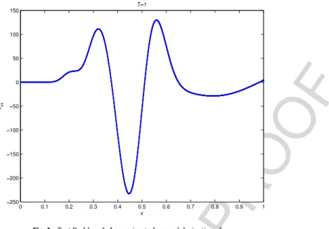
Fig. 1. Test Problem 1. Approximated second derivative ofu.

5. Numerical experiments

1

We have checked experimentally the numerical method. In order to incorporate a more realistic behavior, we introduce

2

a minimum sizeaat which cells divide,xmin

≤

a

<

1. So, we assume that the division ratebvanishes at the interval

[

xmin

,

a

]

.

3

Test problem1. The following experiment shows the optimal rate of convergence obtained with the numerical method.

4

It mirrors a similar one introduced in [13] for the symmetric division case.

5

We takexmin

=

0, anda

=

1₄. We also suppose that there is no cellular death (

µ(

x

)

=

0), and we choose the size-specific

6

growth rate asg

(

x

)

=

0

.

1

(

1

−

x

)

. We take the size-specific division rate function

7

b

(

x

)

=

b1



x

−

1 4



3

,

1

4

≤

x

≤

1

,

8

(coefficientb1is chosen in order to assure that the maximum value ofb

(

x

)

is 1). In order to avoid discontinuities caused by

9

an incompatible initial condition, we take

ϕ

satisfying

ϕ(

0

)

=

ϕ

′

₍

₀

₎

₌

_ϕ

′′

₍

₀

₎

₌

_{0. In this experiment, we opt for}

10

ϕ(

x

)

=















0

,

ifx

∈



0

,

1 8



,

ϕ

1



x

−

1 8



3

(

1

−

x

) ,

ifx

∈



1 8

,

1



,

(5.9)

11

(coefficient

ϕ

₁is chosen in order to assure that the maximum value of

ϕ(

x

)

is 1). Note that this is similar to the third test

12

problem in [13] for the symmetric division case (we assume that initially there are no cells under 1₈). Taking into account

13

the special structure of the equal fission model, there existed numerical difficulties in the numerical simulation due to the

14

lack of smoothness in the solution to the problem: we did not observe the optimal rate of convergence in the numerical

15

approximation. However, as we will see, this test does not provide a remarkable situation in the asymmetric division case.

16

With respect to the partitioning function, as in [17], we take

17

P

(

x

,

y

)

=











1

β(

40

,

40

)

1 y



x y



39



1

−

x

y



39

,

ifx

<

y

,

0

,

ifx

≥

y

,

(5.10)

18

where

β(

x

,

y

)

is the classical Euler beta function.

19

We do not know the analytical solution to the problem therefore, in order to compare, we take the computed

20

approximation with a sufficiently small value of the size stepkas the exact solution. In the experiment we compute such

21

a solution at the final timeT

=

1 withk∗

₌

₄

_.

_8828125e

₋

_{4. If we analyze the (approximated) second derivative of the}

22

computed solution, we observe inFig. 1the required regularity in the hypothesis of the convergence result (as we previously

23

mention, this behavior differs from that of the symmetric division case [13]).

24

InTable 1we present the results obtained with the method for different values of the step size. For eachk, we compare

25

at the final timeTthe computed numerical solutionUN

k, with the representation of the solution corresponding tok ∗_{at the}

Table 1

Test problem 1. Error and numerical convergence order.T=1.

k Error Order

5e−1 1.808892e−2

2.5e−1 5.061369e−3 1.8 1.25e−1 1.252221e−3 2.0 6.25e−2 3.161828e−4 2.1 3.125e−2 8.003949e−5 2.1 1.5625e−2 1.985401e−5 2.0

coarsest grid obtained withk,UN_k∗. Therefore, the second column shows the maximum error at the final time with different 1

step sizes; that is 2

ek

= ∥

UNk

−

U N

k∗

∥

∞

.

3

The third column shows the numerical order of convergence, which we compute with the formula 4

s

=

log

(

e2k

/

ek

)

log

(

2

)

.

5

Results inTable 1clearly confirm the expected second-order of convergence. 6 Test problem2. Now we present the results obtained in order to study the emerging stable size distribution. For the equal 7

fission case, Diekmann et al. [15], proved the existence of a stable size distribution assuming a certain condition of the growth 8

function:g

(

2x

) <

2g

(

x

)

. For the unequal division case, in [17] we have observed the appearance of such asynchronous 9

exponential growth: that is, in the course of time, 10

u

(

x

,

t

)

≈

Ceσtu∗

(

x

),



1

xmin

u∗

(

x

)

dx

=

1

,

(5.11) 11

where

σ

is the Malthusian parameter (intrinsic rate of natural increase), andu∗

₍

_x

₎

_{the stable size distribution. Bothu}∗

₍

_x

₎

12

and

σ

do not depend on the initial condition and only the constantCdepends on

ϕ

. 13

From(5.11)we can write 14

u

(

x

,

t

)



1

xminu

(

x

,

t

)

dx

≈

u∗

(

x

).

(5.12) 15

Then, we can compute an approximation to the stable size distribution by using the numerical solution obtained with 16

the numerical method in the following way: from the numerical solution computed by(3.4)–(3.6), and approximating the 17

integral on the left hand size of(5.12)by means of the composite trapezoidal rule, we can describe the evolution of the 18

frequency of the cell volume distribution which approaches the stable size distributions as 19

U_jn

Q0 k

(

Un

)

≈

U_j∗

.

(5.13) 20

The following simulation reproduces one of the experiments presented in [17]. As in the previous test, we consider the 21

minimum cell-sizexmin

=

0, and the minimum size at which a cell divides asa

=

1₄. Again, we choose the mortality rate 22

µ(

x

)

=

0 (there is no cellular death), and the size-specific growth rateg

(

x

)

=

0

.

1

(

1

−

x

)

. However, this time we use the 23

size-specific division rate function 24

b

(

x

)

=



















0

,

ifx

∈



0

,

1 4



,

g

(

x

)

φ

b

(

x

)

1

−



x

1/4

φ

b

(

s

)

ds

,

ifx

∈



1 4

,

1



,

25

where we have considered that each cell has a stochastically predetermined size at which fission has to occur, which is given 26

by a probability density

φ

b[4]. In this case 27

φ

b

(

x

)

=

λ





















x

−

1 4



3

,

ifx

∈



1 4

,

5 8



,

459 4096

−

9 4



x

−

13 16



2

+

16



x

−

13 16



4

,

ifx

∈



5 8

,

1



,

28

and

λ

=

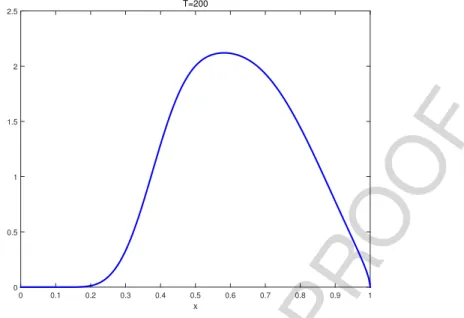
81920

Fig. 2. Test problem 2. Numerical stable size distributionu∗

.

We have carried out an extensive numerical experimentation with different final-timesT and step-sizesk. We observe

1

thatT

=

200 produces a sufficiently long time simulation in order to provide the stable size distribution by means of(5.13).

2

For the step-sizek

=

0

.

01 we obtain the stable size distribution presented inFig. 2, the value of the Malthusian parameter

3

σ

=

0

.

061519, and the computed valueC

=

0

.

440209 associated to the grid restriction of the initial data

ϕ

.

4

6. Conclusions

5

The study of cell populations by means of the use of structured population models, and their numerical simulation, are

6

current and important topics. In this work we consider a size-structured population balance model describing the dynamics

7

of a cell population when the reproduction process takes place by division into two unequal parts. The analytical solution of

8

this problem is difficult to attain in a general situation and numerical approximations are necessary. There are few numerical

9

methods adapted to this problem, and the theoretical studies that would validate them are rare. So it is crucial to design and

10

analyze innovative numerical procedures.

11

In this study we have proposed a new and efficient numerical method in order to attain the solution to this model. It is

12

an extension of the one given in [13] for the even case, which could be seen as a particular model when the partitioning

13

function is a Dirac delta. The uneven model seems to be more realistic and it does not introduce a lack of smoothness in

14

the solution. However, the birth term in the equation involves an integral term that must be approximated by means of a

15

suitable quadrature rule. This issue requires a more expensive, slower and harder numerical integration. However, we have

16

improved the efficiency of the numerical procedure by using a suitable subgrid of the natural grid in the quadrature rule.

17

We have carried out a demonstration of the second-order convergence of the approximate solution to the exact one

18

under suitable smoothness hypotheses of the vital functions and the exact solution, and we have corroborated this optimal

19

rate experimentally.

20

Finally, this numerical method is revealed as a valuable tool for the analysis and approximation of the stable size

distri-21

bution of the model.

22

Acknowledgments

23

This work was supported in part by project MTM2014-56022-C2-2-P of the Spanish Ministerio de Economía y

Compet-24

itividad and European FEDER Funds, and by project VA191U13 of the Consejería de Educación, JCyL.

25

References

26

[1] G.I. Bell, E.C. Anderson, Cell growth and division: I. A mathematical model with applications to cell volume distributions in mammalian suspension cultures, Biophys. J. 7 (1967) 329–351.

27

[2] A.G. Fredrickson, D. Ramkrishna, H.M. Tsuchiya, Statistics and dynamics of procaryotic cell populations, Math. Biosci. 1 (1967) 327–374.

28

[3] A. Lasota, M.C. Mackey, Probabilistic Properties of Deterministic Systems, Cambridge University Press, London, 1985.

29

[4] J.A.J. Metz, O. Diekmann (Eds.), The Dynamics of Physiologically Structured Populations, in: Lect. Notes Biomath., vol. 68, Springer-Verlag, New York, 1986.

30

[5] B. Perthame, Transport Equations in Biology, Birkhäuser, Basel, Switzerland, 2007.

31

[6] R. Borges, A. Calsina, S. Cuadrado, Oscillations in a molecular structured cell population model, Nonlinear Anal. RWA 12 (2011) 1911–1922.

[7] S. Fadda, A. Cincotti, G. Cao, A novel population balance model to investigate the kinetics of in vitro cell proliferation: Part I. Model development, Biotechnol. Bioeng. 109 (2012) 772–781.

1

[8] S. Fadda, A. Cincotti, G. Cao, A novel population balance model to investigate the kinetics of in vitro cell proliferation: Part II. Numerical solution, parameters, determination, and model outcomes, Biotechnol. Bioeng. 109 (2012) 782–796.

2

[9] K. Spetsieris, K. Zygourakis, Single-cell behavior and population heterogeneity: Solving an inverse problem to compute the intrinsic physiological state functions, J. Biotechnol. 158 (2012) 80–90.

3

[10] D. Ramkrishna, Statistical models of cell populations, in: Adv. Biochem. Eng., vol. 11, Springer, Berlin, 1979, pp. 1–47. 4

[11] L. Abia, O. Angulo, J.C. López-Marcos, Size-structured population dynamics models and their numerical solutions, Discrete Contin. Dyn. Syst. Ser. B 4 (2004) 1203–1222.

5

[12] L. Abia, O. Angulo, J.C. López-Marcos, Age-structured population dynamics models and their numerical solutions, Ecol. Model. 188 (2005) 112–136. 6

[13] O. Angulo, J.C. López-Marcos, M.A. López-Marcos, A second-order method for the numerical integration of a size-structured cell population model, 7

Abstr. Appl. Anal. 549168 (2015) 1–8.http://dx.doi.org/10.1155/2015/549168. 8

[14] O. Arino, A survey of structured cell population dynamics, Acta Biotheor. 43 (1995) 3–25. 9

[15] O. Diekmann, H.J.A.M. Heijmans, H.R. Thieme, On the stability of the cell size distribution, J. Math. Biol. 19 (1984) 227–248. 10

[16] J.M. Cushing, An Introduction to Structured Population Dynamics, in: CMB-NSF Regional Conference Series in Applied Mathematics, vol. 71, SIAM, Philadelphia, 1998.

11

[17] O. Angulo, J.C. López-Marcos, M.A. López-Marcos, A semi-Lagrangian method for a cell population model in a dynamical environment, Math. Comput. Modelling 57 (2013) 1860–1866.