A Second Order Method for the Numerical Integration of a Size Structured Cell Population Model

(1)

Research Article

A Second-Order Method for the Numerical Integration of

a Size-Structured Cell Population Model

O. Angulo,

1

J. C. López-Marcos,

2

and M. A. López-Marcos

2

1_{Departamento de Matem´atica Aplicada, ETSIT, Universidad de Valladolid, Paseo de Bel´en 15, 47011 Valladolid, Spain}

2_{Departamento de Matem´atica Aplicada, Facultad de Ciencias, Universidad de Valladolid, Paseo de Bel´en 7, 47011 Valladolid, Spain}

Correspondence should be addressed to M. A. L´opez-Marcos; malm@mac.uva.es

Received 30 December 2014; Revised 27 March 2015; Accepted 6 April 2015

Academic Editor: Francisco Solis

Copyright © 2015 O. Angulo et al. This is an open access article distributed under the Creative Commons Attribution License, which permits unrestricted use, distribution, and reproduction in any medium, provided the original work is properly cited.

We consider the numerical integration of a size-structured cell population model. We propose a new second-order numerical method to attain its solution. The scheme is analyzed and the optimal rate of convergence is derived. We show experimentally the predicted accuracy of the scheme.

1. Introduction

Population models are important tools in life sciences. Several types of them are commonly employed in the literature, and population balance models are one of the most applied models. These models describe the evolution of the pop-ulation by considering that it is structured by means of several physiological characteristics. Their main features can be found in [1–3] and references therein. Cell populations can also be described in this framework. They are structured,

inter alia, by the age spent in the cell cycle, cell size, or

other features such as the content of groups of proteins called cyclin and intensity of certain markers. For a reference, we can mention recent literature which describes very different problems such as oscillations in a cyclin content structured model [4], the growth of yeast populations in morpholog-ically structured ones [5, 6], or gene expression in a label-structured population [7]. References therein also provide information about the study of cell populations by means of structured models. We consider the linear size-structured population model proposed by Diekmann et al. [8]. This is a starting point in the study of more complex problems. In this model, cell mitosis happens in a symmetric way and a cell does not divide until it reaches a minimal size𝑎 > 0. This means that there is a positive minimum cell size. However, we consider that there must be a maximal size, normalized

to𝑥 = 1, at which point every cell might divide or die. The model we study is given by a conservation law

𝑢_𝑡(𝑥, 𝑡) + (𝑔 (𝑥) 𝑢 (𝑥, 𝑡))_𝑥= − 𝜇 (𝑥) 𝑢 (𝑥, 𝑡) − 𝑏 (𝑥) 𝑢 (𝑥, 𝑡) + 4𝑏 (2𝑥) 𝑢 (2𝑥, 𝑡) ,

(1)

𝑎/2 < 𝑥 < 1,𝑡 > 0, a boundary condition

𝑢 (𝑎₂, 𝑡) = 0, 𝑡 > 0, (2)

and an initial size distribution

𝑢 (𝑥, 0) = 𝜑 (𝑥) , 𝑎₂ ≤ 𝑥 ≤ 1. (3)

The independent variables𝑥and𝑡represent size and time, respectively. The dependent variable𝑢(𝑥, 𝑡)is the size-specific density of cells with size𝑥at time𝑡and we assume that the size of any individual varies according to the following ordinary differential equation:

𝑑𝑥

𝑑𝑡 = 𝑔 (𝑥) . (4)

The nonnegative functions𝑔,𝜇, and𝑏represent the growth, mortality, and division rate, respectively. These are usually

(2)

called the vital functions and define the life history of the individuals. Note that all of them depend on the size 𝑥 (the internal structuring variable). We should point out that, in (1), the reproduction process into two equal parts has been considered in the two terms in which the division rate appears. Here, we should note that the term4𝑏(2𝑥)𝑢(2𝑥, 𝑡) is interpreted as zero whenever 𝑥 > 1/2. We perform this feature with the use of functions 𝑢 and 𝑏 extended with the value zero on the interval [1, 2]. Condition (2)

reflects that cells with a size less than𝑎/2cannot exist and is a consequence of the fact that cells only divide after the minimal size𝑎 > 0.

In accordance with accepted biological wisdom, there exists a maximum size. This means that cells will divide or die with probability one before reaching it. Thus, if we consider the survival property, that is, the probability that an individual of size𝑥₀reaches size𝑥,

Π (𝑥) =exp(− ∫

𝑥

𝑥0

𝜇 (𝑠) + 𝑏 (𝑠) 𝑔 (𝑠) 𝑑𝑠) ,

𝑎

2 ≤ 𝑥0≤ 𝑥 < 1,

(5)

the hypothesis of considering a maximum size implies that lim_{𝑥 → 1}−Π(𝑥) = 0. One of the forms in which this fact could be reflected consists of taking into account the growth functions introduced by Von Bertalanffy. These kinds of functions satisfy∫_𝑥1

0(𝑑𝑠/𝑔(𝑠)) = ∞, which is enough to verify the required condition whenever 𝜇and 𝑏 are positive and bounded functions. Note that if𝑔is a continuous function defined in[𝑎/2, 1], then this hypothesis implies that𝑔(1) = 0. Moreover, the solution to the problem must satisfy𝑢(1, 𝑡) = 0,

𝑡 > 0, because we suppose that initially there are no cells of maximum size [2].

In general, physiologically structured population models are difficult to solve. Although theoretical properties of the models such as existence, uniqueness, smoothness of solutions, and long-time behaviour (with the study of steady states and their stability) could be studied without a solution expression, the knowledge of their qualitative or quantitative behaviour in a more tangible way is sometimes necessary. Therefore, numerical methods provide a valuable tool to obtain such information. In the case of general structured population models, many numerical methods have been proposed to solve them (see [9,10] and references therein), and the difficulties found in their convergence analysis can be observed in [11], for instance.

In the case of population balance models such as (1)–

(3), Liou et al. [12] proposed an alternative procedure for their solution based on a successive generations approach that provides analytical solutions in some cases. However, numer-ical integration may be necessary for more complicated situations. Mantzaris et al. [13] presented a finite difference scheme and Angulo and L´opez-Marcos [14] a characteristic curve scheme with the first convergence analysis. However, until that moment, a maximum size for the cells was not considered. For the case of a bounded size interval, the works of Mantzaris et al. [15–17] provided a broad comparison of numerical methods based on finite differences and spectral and finite elements method, respectively. In their work,

the authors compared the efficiency of the methods presented but they did not demonstrate their convergence and did not pay attention to either the compatibility of the initial and boundary conditions or the discontinuities caused by the maximum size. Note that the lack of smoothness properties of the solution would negatively affect the efficiency of such higher order methods. In our previous work [18], we formu-lated two first-order numerical procedures, a finite difference scheme and a characteristics method, and analyzed com-pletely their convergence. The work supplied a detailed trac-ing of the different discontinuities aristrac-ing in the simulation.

When selecting a numerical method, efficiency must be taken into account [19]. In general, on a long-time integration (e.g., see a study of the stable size distribution in [18]), the use of methods that preserve some of the qualitative properties of the solution can perform better and, thus, characteristic curves methods would be good candidates. In this paper, we consider a novel characteristics method based on the discretization of the integral representation of the solution to the problem along the characteristics lines. This procedure was previously used in [18] for this problem, obtaining a valuable first-order method. Here, in order to produce a second-order scheme, we consider a different discretization of the integral representation to the solution. Second-order methods maintain good compromise between the required smoothness of the vital functions based on realistic biological data and the efficiency of the numerical schemes. Never-theless, this alternative discretization produces an implicit numerical method that, in principle, increases the stability property but also the computational cost. However, due to the special structure of the problem, a suitable implemen-tation of the numerical method provides a cheaper explicit procedure.

In Section 2, we describe the numerical method to

approximate the solution to(1)–(3)and comment upon the efficient implementation being used. Section 3 is devoted to the convergence analysis of the method. In Section 4, we present some numerical experiments which confirm the theoretical results and describe the performance of the numerical method in different situations related to the lack of smoothness properties of the vital functions and the solution.

2. Numerical Method

As we mentioned in Section 1, there are some schemes proposed to obtain the solution to(1)–(3). Most of them are of first-order convergence. On the one hand, this convergence property produces a lack of efficiency which can be reduced with higher order methods. On the other hand, the smooth-ness of the solution to (1)–(3) is not as high as these last schemes demand. However, second-order methods present a good balance: they enhance the efficiency even with a lack of regular data.

Here, we introduce an overall second-order numerical method which integrates the problem along the characteristic curves. It employs a theoretical representation of the solution to(1)–(3)whose framework was introduced in [18]. There-fore, following such work, we define𝜇∗(𝑥) = 𝑔󸀠(𝑥) + 𝜇(𝑥) +

(3)

takes the value𝑥_∗at the time instant𝑡_∗of(1). It is the solution to the following initial value problem:

𝑑

𝑑𝑡𝑥 (𝑡; 𝑡∗, 𝑥∗) = 𝑔 (𝑥 (𝑡; 𝑡∗, 𝑥∗)) , 𝑡 > 𝑡∗,

𝑥 (𝑡_∗; 𝑡_∗, 𝑥_∗) = 𝑥_∗.

(6)

In this way, the solution to(1)is given by

𝑢 (𝑥 (𝑡; 𝑡_∗, 𝑥_∗) , 𝑡) = 𝑢 (𝑥_∗, 𝑡_∗)

⋅exp{− ∫𝑡

𝑡∗

𝜇∗(𝑥 (𝜏; 𝑡_∗, 𝑥_∗)) 𝑑𝜏}

+ ∫𝑡

𝑡∗

exp{− ∫

𝑡

𝜏𝜇 ∗_{(𝑥 (𝑠; 𝑡}

∗, 𝑥∗)) 𝑑𝑠}

⋅ 4𝑏 (2𝑥 (𝜏; 𝑡_∗, 𝑥_∗))

⋅ 𝑢 (2𝑥 (𝜏; 𝑡_∗, 𝑥_∗) , 𝜏) 𝑑𝜏, 𝑡 ≥ 𝑡_∗.

(7)

Note that, in this new layout, we have to solve two types of problems: the integration of the equation that defines the characteristic curves(6)and the solution to (7)which provides the solution to the problem along the characteristics. We use discretization procedures in order to solve them.

We consider the numerical integration of model(1)–(3)

along the time interval[0, 𝑇]. Thus, given a positive integer

𝑁, we define𝑘 = 𝑇/𝑁and introduce the discrete time levels

𝑡𝑛 _{= 𝑛𝑘}_,_{0 ≤ 𝑛 ≤ 𝑁}_{. We begin with the integration of}₍₆₎

which provides the grid on the space variable (size) of the method. This grid is nonuniform and invariant with time, because the growth rate function is, explicitly, independent of the time variable. However, note that it depends on time implicitly conditioned on cell size. It is usually called the

natural grid[9]. In this work, we approximate such a grid by

using a second-order scheme for the numerical integration of

(6). More precisely, the modified Euler method provides the following approximation to the natural grid:

𝑥₀=𝑎₂,

𝑥_𝑗+1= 𝑥_𝑗+𝑘

2( 𝑔 ( 𝑥𝑗) + 𝑔 ( 𝑥𝑗+ 𝑘𝑔 ( 𝑥𝑗))) , 0 ≤ 𝑗 ≤ 𝐽 − 1.

(8)

Integer𝐽represents the index of the last grid point computed at the size interval and is chosen to satisfy the condition𝐾₀𝑘 ≤

1 − 𝑥_𝐽 ≤ 𝐾₁𝑘, with𝐾₀and𝐾₁being suitable constants (we refer to [9] for further details). Note that the points(𝑥_𝑗, 𝑡_𝑛) and(𝑥_𝑗+1, 𝑡_𝑛+1),0 ≤ 𝑗 ≤ 𝐽 − 1,0 ≤ 𝑛 ≤ 𝑁 − 1, belong to the same numerical characteristic curve. Finally, we fix the last grid point𝑥_𝐽+1 = 1.

Then, denoting 𝑢𝑛_𝑗 = 𝑢(𝑥_𝑗, 𝑡𝑛), 0 ≤ 𝑗 ≤ 𝐽 + 1, 0 ≤

𝑛 ≤ 𝑁, let 𝑈_𝑗𝑛 be a numerical approximation to 𝑢𝑛_𝑗. We propose a one-step method in order to obtain it. Therefore, starting from an approximation to the initial data(3)of the problem, for example, the grid restriction of the function𝜑,

the numerical solution at a new time level is described in terms of the previous one. Such a general step is obtained by means of the following second-order discretization of(7): the integrals are approached by the trapezoidal quadrature rule. For0 ≤ 𝑛 ≤ 𝑁 − 1,

𝑈𝑛+1

𝑗+1 =exp{−𝑘₂(𝜇∗(𝑥𝑗) + 𝜇∗(𝑥𝑗+1))}

⋅ ( 𝑈_𝑗𝑛+ 2𝑘𝑏 ( 2𝑥𝑗) 𝑈𝑛2⋅𝑗)

+ 2𝑘𝑏 (2𝑥𝑗+1) 𝑈𝑛+12⋅(𝑗+1), 𝑗 = 0, . . . , 𝐽 − 1.

(9)

In the previous expression,𝑈𝑛_2⋅𝑗and𝑈𝑛+1_2⋅(𝑗+1)represent approx-imations to the solutions at sizes2𝑥_𝑗and2𝑥_𝑗+1(not included in the discrete grid) and times𝑡𝑛 and𝑡𝑛+1, respectively. So, in order to keep the second order, we compute them by linear interpolation based on the nearest grid points. More precisely, for the computation of 𝑈𝑚_2⋅𝑙, approximation to the solution at2𝑥_𝑙, and time 𝑡𝑚, first we look for the index 𝑀so that

𝑥_𝑀−1< 2𝑥_𝑙≤ 𝑥_𝑀. Thus,

𝑈𝑚_2⋅𝑙={{_{_{ {

𝑈_𝑀−1𝑚 +𝑈_𝑥𝑀𝑚 − 𝑈𝑀−1𝑚

𝑀− 𝑥𝑀−1 (2𝑥𝑙− 𝑥𝑀−1) , if 2𝑥𝑙< 1,

0, if 2𝑥_𝑙≥ 1.

(10)

Obviously, the approximating values at the minimum and maximum sizes are

𝑈₀𝑛+1= 𝑈_𝐽+1𝑛+1= 0. (11)

The numerical procedure seems to be implicit. However, if we compute the approximations at the new time level𝑡𝑛+1 downwards (i.e., first𝑈_𝐽+1𝑛+1using(11), then𝑈_𝑗+1𝑛+1from𝐽 − 1to

0using(9), and finally𝑈₀𝑛+1using(11)), it results in an explicit procedure. The reason is that the right hand side values in(9)

corresponding to the time𝑡𝑛+1are either zero or previously computed.

3. Convergence Analysis

In this section, we carry out the convergence analysis of the scheme. It is based on the properties of consistency and stability of the method. Henceforth,𝐶will denote a positive constant which is independent of𝑘,𝑛(0 ≤ 𝑛 ≤ 𝑁) and𝑗 (0 ≤ 𝑗 ≤ 𝐽 + 1);𝐶possibly has different values in different places.

The local discretization error is given by the following

equation:

𝜏_𝑗+1𝑛+1= 1

𝑘(𝑢𝑛+1𝑗+1−exp{−𝑘₂(𝜇∗(𝑥𝑗) + 𝜇∗(𝑥𝑗+1))}

⋅ ( 𝑢𝑛_𝑗 + 2𝑘𝑏 ( 2𝑥_𝑗) 𝑢𝑛_2⋅𝑗) − 2𝑘𝑏 (2𝑥_𝑗+1) 𝑢𝑛+1_2⋅(𝑗+1)) ,

0 ≤ 𝑗 ≤ 𝐽 − 1, 0 ≤ 𝑛 ≤ 𝑁 − 1.

(4)

Lemma 1. Let𝑔be three times continuously differentiable; let

functions𝜇,𝑏, and𝑢be two times continuously differentiable.

Thus, as𝑘 → 0, the following estimates hold:

󵄨󵄨󵄨󵄨

󵄨𝜏𝑗+1𝑛+1󵄨󵄨󵄨󵄨_{󵄨 = 𝑂 ( 𝑘}2) , 0 ≤ 𝑗 ≤ 𝐽 − 1, 0 ≤ 𝑛 ≤ 𝑁 − 1. (13)

Proof. From(12)and(7), by adding and subtracting suitable

terms in the expression of the local discretization error, we obtain the following bound:

󵄨󵄨󵄨󵄨

󵄨𝜏𝑗+1𝑛+1󵄨󵄨󵄨󵄨_{󵄨 ≤} 1_𝑘󵄨󵄨󵄨󵄨_󵄨𝑢𝑗+1𝑛+1− 𝑢 ( 𝑥 ( 𝑡𝑛+1; 𝑥𝑗, 𝑡𝑛) , 𝑡𝑛+1)󵄨󵄨󵄨󵄨󵄨

+1 𝑘󵄨󵄨󵄨󵄨󵄨𝑢𝑛𝑗󵄨󵄨󵄨󵄨_󵄨󵄨󵄨󵄨󵄨󵄨󵄨󵄨󵄨

󵄨exp{− ∫

𝑡𝑛+1

𝑡𝑛

𝜇∗( 𝑥 ( 𝜏; 𝑡_𝑛, 𝑥_𝑗)) 𝑑𝜏}

−exp{−𝑘

2(𝜇∗(𝑥𝑗)

+ 𝜇∗( 𝑥 ( 𝑡_𝑛+1; 𝑡_𝑛, 𝑥_𝑗)))}󵄨󵄨󵄨󵄨_{󵄨󵄨󵄨󵄨} 󵄨 +1_𝑘󵄨󵄨󵄨󵄨_󵄨𝑢𝑛_𝑗󵄨󵄨󵄨󵄨_󵄨exp{−𝑘

2𝜇∗(𝑥𝑗)}

⋅󵄨󵄨󵄨󵄨_{󵄨󵄨󵄨󵄨}exp{−𝑘

2𝜇∗( 𝑥 ( 𝑡𝑛+1; 𝑡𝑛, 𝑥𝑗))}

−exp{−𝑘

2𝜇∗(𝑥𝑗+1)}󵄨󵄨󵄨󵄨󵄨󵄨󵄨󵄨

+4_𝑘󵄨󵄨󵄨󵄨_{󵄨󵄨󵄨󵄨} 󵄨∫

𝑡𝑛+1

𝑡𝑛

exp{− ∫𝑡𝑛+1

𝜏 𝜇

∗_{( 𝑥 ( 𝑠; 𝑡}

𝑛, 𝑥𝑗)) 𝑑𝑠}

⋅ 𝑏 (2𝑥 (𝜏; 𝑡_𝑛, 𝑥_𝑗))

⋅ 𝑢 (2𝑥 (𝜏; 𝑡𝑛, 𝑥𝑗) , 𝜏) 𝑑𝜏

−𝑘

2(exp{− ∫

𝑡𝑛+1

𝑡𝑛

𝜇∗( 𝑥 ( 𝑠; 𝑡_𝑛, 𝑥_𝑗)) 𝑑𝑠}

⋅ 𝑏 ( 2𝑥𝑗) 𝑢 ( 2𝑥𝑗, 𝑡𝑛)

+ 𝑏 (2𝑥 (𝑡_𝑛+1; 𝑡_𝑛, 𝑥_𝑗))

⋅ 𝑢 (2𝑥 (𝑡_𝑛+1; 𝑡_𝑛, 𝑥_𝑗) , 𝑡_𝑛+1))󵄨󵄨󵄨󵄨_{󵄨󵄨󵄨󵄨} 󵄨

+ 2󵄨󵄨󵄨󵄨_{󵄨󵄨󵄨󵄨}

󵄨exp{− ∫

𝑡𝑛+1

𝑡𝑛

𝜇∗( 𝑥 ( 𝑠; 𝑡_𝑛, 𝑥_𝑗)) 𝑑𝑠}

−exp{−𝑘

2(𝜇∗(𝑥𝑗) + 𝜇∗( 𝑥 ( 𝑡𝑛+1; 𝑡𝑛, 𝑥𝑗)))}󵄨󵄨󵄨󵄨󵄨󵄨󵄨󵄨_󵄨 ⋅ 󵄨󵄨󵄨󵄨󵄨𝑏(2𝑥𝑗) 𝑢 (2𝑥𝑗, 𝑡𝑛)󵄨󵄨󵄨󵄨󵄨

+ 2exp{−𝑘

2𝜇∗(𝑥𝑗)}

⋅󵄨󵄨󵄨󵄨_{󵄨󵄨󵄨󵄨}exp{−𝑘

2𝜇∗( 𝑥 ( 𝑡𝑛+1; 𝑡𝑛, 𝑥𝑗))}

−exp{−𝑘

2𝜇∗(𝑥𝑗+1)}󵄨󵄨󵄨󵄨󵄨󵄨󵄨󵄨

⋅ 󵄨󵄨󵄨󵄨󵄨𝑏(2𝑥𝑗) 𝑢 (2𝑥𝑗, 𝑡𝑛)󵄨󵄨󵄨󵄨󵄨

+ 2exp{−𝑘

2(𝜇∗(𝑥𝑗) + 𝜇∗(𝑥𝑗+1))} 󵄨󵄨󵄨󵄨󵄨𝑏(2𝑥𝑗)󵄨󵄨󵄨󵄨󵄨 ⋅ 󵄨󵄨󵄨󵄨󵄨𝑢(2𝑥𝑗, 𝑡𝑛) − 𝑢𝑛2⋅𝑗󵄨󵄨󵄨󵄨_󵄨

+ 󵄨󵄨󵄨󵄨󵄨𝑏(2𝑥(𝑡𝑛+1; 𝑡𝑛, 𝑥𝑗)) − 𝑏 (2𝑥𝑗+1)󵄨󵄨󵄨󵄨󵄨

⋅ 󵄨󵄨󵄨󵄨󵄨𝑢(2𝑥(𝑡𝑛+1; 𝑡𝑛, 𝑥𝑗) , 𝑡𝑛+1)󵄨󵄨󵄨󵄨󵄨

+ 󵄨󵄨󵄨󵄨󵄨𝑏(2𝑥𝑗+1)󵄨󵄨󵄨󵄨󵄨

⋅ 󵄨󵄨󵄨󵄨󵄨𝑢(2𝑥(𝑡𝑛+1; 𝑡𝑛, 𝑥𝑗) , 𝑡𝑛+1) − 𝑢 ( 2𝑥𝑗+1, 𝑡𝑛+1)󵄨󵄨󵄨󵄨󵄨

+ 󵄨󵄨󵄨󵄨󵄨𝑏(2𝑥𝑗+1)󵄨󵄨󵄨󵄨󵄨󵄨󵄨󵄨󵄨_{󵄨𝑢 ( 2𝑥}𝑗+1, 𝑡𝑛+1) − 𝑢𝑛+12⋅(𝑗+1)󵄨󵄨󵄨󵄨_{󵄨 ,}

(14)

0 ≤ 𝑗 ≤ 𝐽 − 1,0 ≤ 𝑛 ≤ 𝑁 − 1. Now, taking into account the convergence properties of the trapezoidal quadrature rule, the modified Euler method, the interpolation procedure, and the assumed regularity of functions𝑔,𝜇,𝑏, and𝑢, we obtain the estimate (remember that 𝑢 and 𝑏 must be considered smooth in their extended domains).

In the following result, we prove the convergence of the numerical method. We denote the error produced by the numerical approximation by

e𝑛 = ( 𝑒𝑛₀, . . . , 𝑒𝑛_𝐽, 𝑒_𝐽+1𝑛 ) , 𝑒_𝑗𝑛= 𝑢𝑛_𝑗− 𝑈_𝑗𝑛, 0 ≤ 𝑗 ≤ 𝐽 + 1,

(15)

0 ≤ 𝑛 ≤ 𝑁, where𝑢𝑛_𝑗 are the nodal values of the theoretical solution and𝑈_𝑗𝑛are the numerical approximations obtained by means of the numerical method. And

𝑒𝑚_2⋅𝑙={_{ {

𝑢𝑚_2⋅𝑙− 𝑈𝑚_2⋅𝑙, 𝑥_𝑀−1< 2𝑥_𝑙≤ 𝑥_𝑀≤ 1,

0, 2𝑥_𝑙≥ 1, (16)

0 ≤ 𝑙 ≤ 𝐽,0 ≤ 𝑚 ≤ 𝑁.

Theorem 2. Under the hypotheses of Lemma 1, if ‖e0‖_∞ =

𝑂(𝑘2₎_{, as}_{𝑘 → 0}_{, then}

󵄩󵄩󵄩󵄩e𝑛󵄩󵄩󵄩󵄩_∞≤ 𝐶𝑘2, 0 ≤ 𝑛 ≤ 𝑁. (17)

Proof. From(9)and(12), we have

𝑒𝑛+1_𝑗+1 =exp{−𝑘

2(𝜇∗(𝑥𝑗) + 𝜇∗(𝑥𝑗+1))} (𝑒𝑛𝑗+ 2𝑘𝑏 ( 2𝑥𝑗) 𝑒𝑛2⋅𝑗)

− 2𝑘𝑏 (2𝑥𝑗+1) 𝑒𝑛+12⋅(𝑗+1)+ 𝑘𝜏𝑗+1𝑛+1,

(18)

0 ≤ 𝑗 ≤ 𝐽 − 1, 0 ≤ 𝑛 ≤ 𝑁 − 1. Taking into account the smoothness properties of the functions𝜇∗and𝑏, we arrive at

󵄨󵄨󵄨󵄨

󵄨𝑒𝑛+1𝑗+1󵄨󵄨󵄨󵄨_{󵄨 ≤ (1 + 𝐶𝑘)}󵄨󵄨󵄨󵄨_󵄨𝑒𝑛𝑗󵄨󵄨󵄨󵄨_{󵄨 + 𝐶𝑘 (}󵄩󵄩󵄩󵄩e𝑛󵄩󵄩󵄩󵄩∞+ 󵄩󵄩󵄩󵄩󵄩e𝑛+1󵄩󵄩󵄩󵄩_󵄩∞) + 𝑘 󵄨󵄨󵄨󵄨󵄨𝜏𝑗+1𝑛+1󵄨󵄨󵄨󵄨󵄨 ,

(5)

0 ≤ 𝑗 ≤ 𝐽 − 1,0 ≤ 𝑛 ≤ 𝑁 − 1, and

󵄨󵄨󵄨󵄨

󵄨𝑒𝑛+1𝑗+1󵄨󵄨󵄨󵄨_{󵄨 ≤ (1 + 𝐶𝑘)}󵄩󵄩󵄩󵄩e𝑛󵄩󵄩󵄩󵄩∞+ 𝐶𝑘 󵄩󵄩󵄩󵄩󵄩e𝑛+1󵄩󵄩󵄩󵄩󵄩∞+ 𝑘 󵄩󵄩󵄩󵄩󵄩𝜏𝑛+1󵄩󵄩󵄩󵄩󵄩∞, (20)

0 ≤ 𝑗 ≤ 𝐽 − 1,0 ≤ 𝑛 ≤ 𝑁 − 1. Then, by means of a recursive argument, we obtain

󵄨󵄨󵄨󵄨

󵄨𝑒𝑛𝑗󵄨󵄨󵄨󵄨_{󵄨 ≤ (1 + 𝐶𝑘)}𝑛󵄩󵄩󵄩󵄩_󵄩e0󵄩󵄩󵄩󵄩_󵄩_∞+ 𝐶𝑘 𝑛

∑

𝑙=1

(1 + 𝐶𝑘)𝑛−𝑙󵄩󵄩󵄩󵄩_󵄩e𝑙󵄩󵄩󵄩󵄩_󵄩_∞

+ 𝑘∑𝑛

𝑙=1

(1 + 𝐶𝑘)𝑛−𝑙󵄩󵄩󵄩󵄩_󵄩𝜏𝑙󵄩󵄩󵄩󵄩_󵄩_∞,

(21)

1 ≤ 𝑗 ≤ 𝐽,1 ≤ 𝑛 ≤ 𝑁. Therefore,

󵄩󵄩󵄩󵄩e𝑛󵄩󵄩󵄩󵄩_∞_{≤ 𝐶 {󵄩󵄩󵄩󵄩󵄩}e0󵄩󵄩󵄩󵄩_󵄩_∞+ 𝑘∑𝑛

𝑙=1󵄩󵄩󵄩󵄩󵄩

e𝑙󵄩󵄩󵄩󵄩_󵄩_∞+ 𝑘∑𝑛

𝑙=1󵄩󵄩󵄩󵄩󵄩𝜏 𝑙󵄩󵄩󵄩󵄩

󵄩∞} , (22)

1 ≤ 𝑛 ≤ 𝑁. By the discrete Gronwall lemma and using(13), we arrive at

󵄩󵄩󵄩󵄩e𝑛󵄩󵄩󵄩󵄩_∞_{≤ 𝐶 󵄩󵄩󵄩󵄩󵄩}e0󵄩󵄩󵄩󵄩_󵄩_∞+ 𝑂 ( 𝑘2) , (23)

0 ≤ 𝑛 ≤ 𝑁, and the estimate holds.

4. Numerical Results

Now, we present some different experiments in order to test the numerical method. We consider the minimum size at which a cell divides as𝑎 = 1/4. We suppose that there is no cellular death. Therefore,𝜇(𝑥) = 0, and we choose the size-specific growth rate as𝑔(𝑥) = 0.1(1 − 𝑥).

Test Problem 1. In the first experiment, we take the

size-specific division rate function

𝑏 (𝑥) = 𝑏0(𝑥 −1₄) 3

(1 − 𝑥)3, 1₄ ≤ 𝑥 ≤ 1. (24)

We consider that the function vanishes out of interval[1/4, 1]. Coefficient𝑏₀is chosen in order to ensure that the maximum value of𝑏(𝑥)is1. Note that the extended function is two times continuously differentiable.

In order to avoid discontinuities caused by an incompat-ible initial condition, we take𝜑satisfying𝜑(1/8) = 𝜑󸀠(1/8) =

𝜑󸀠󸀠_{(1/8) = 0}_{. In this first experiment, we opt for}

𝜑 (𝑥) = 𝜑0(𝑥 −1₈) 3

(1 − 𝑥)3, 1

8 ≤ 𝑥 ≤ 1, (25)

with the corresponding extension out of the interval[1/8, 1]. Coefficient𝜑₀is chosen in order to ensure that the maximum value of𝜑(𝑥)is1.

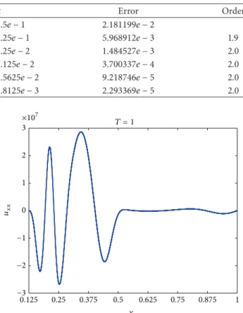
We do not know the analytical solution to the problem, so, in order to compare, we take as an exact solution the computed approximation with a sufficiently small value of the size step𝑘. In the experiment, we compute the solution at the final time𝑇 = 1with𝑘∗ = 4.8828125𝑒 − 4. If we analyze the (approximated) second derivative of the computed solution,

Table 1: Test Problem 1. Error and numerical convergence order.

𝑇 = 1.

𝑘 Error Order

2.5𝑒 − 1 2.181199𝑒 − 2

1.25𝑒 − 1 5.968912𝑒 − 3 1.9

6.25𝑒 − 2 1.484527𝑒 − 3 2.0

3.125𝑒 − 2 3.700337𝑒 − 4 2.0

1.5625𝑒 − 2 9.218746𝑒 − 5 2.0

7.8125𝑒 − 3 2.293369𝑒 − 5 2.0

0.125 0.25 0.375 0.5 0.625 0.75 0.875 1

0 1 2 3

x T = 1

×107

−3 −2 −1 uxx

Figure 1: Test Problem 1. Approximated second derivative of𝑢.

we observe the required regularity in the hypotheses of the convergence result (seeFigure 1).

In Table 1, we present the results obtained with the

method for different values of the step size. For each𝑘, we compare at the final time 𝑇 the numerical solution being computed,U𝑁_𝑘, with the representation of the numerical solu-tion corresponding to𝑘∗at the coarsest grid obtained with𝑘,

U𝑁

𝑘∗. The second column inTable 1shows the maximum error at the different discrete sizes; that is,

𝑒_𝑘_{= 󵄩󵄩󵄩󵄩󵄩}U𝑁_𝑘 −U𝑁_𝑘∗󵄩󵄩󵄩󵄩_󵄩

∞. (26)

The third column shows the numerical order of convergence, which we compute with the formula

𝑠 = log(𝑒2𝑘/𝑒𝑘)

log(2) . (27)

Results in Table 1clearly confirm the expected second-order of convergence.

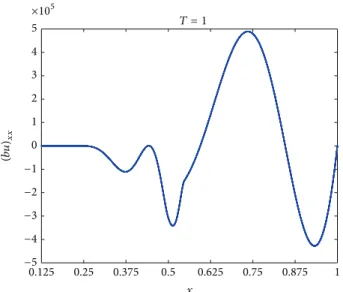
Test Problem 2.In the second experiment, we take a

size-specific division rate function not satisfying the smoothness required in the assumptions of the convergence result. For example,

𝑏 (𝑥) = 𝑏1(𝑥 −1₄) 3

(6)

0.125 0.25 0.375 0.5 0.625 0.75 0.875 1 0

1 2 3 4

5 T = 1

×105

−5 −4 −3 −2 −1

x

(b

u)xx

Figure 2: Test Problem 2. Approximated second derivative of𝑏𝑢.

Again, we consider that 𝑏(𝑥) vanishes out of the interval

[1/4, 1]. Coefficient𝑏₁ is chosen in order to ensure that the maximum value of𝑏(𝑥)is 1. Note that, now, this extended function is discontinuous.

Assuming the same initial data (25)as in the previous experiment, we obtain the results presented inTable 2. Again, we observe a second-order convergence.

Perhaps these numerical results can be explained by tak-ing into account that the (approximated) second derivative of the product𝑏𝑢is continuous as can be observed inFigure 2. A detailed revision of the convergence result (which we do not include for the sake of simplicity) allows us to ensure the same estimative by relaxing the hypothesis, assuming that the extension of the product𝑏𝑢 is two times continuously differentiable instead of the extension of𝑏.

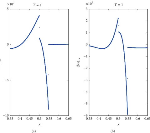
Test Problem 3.We take the size-specific division rate function

(28)of the previous experiment not satisfying the smoothness assumptions of the convergence result. But now, we consider the following initial data (producing a nonsufficiently smooth solution, as we will show),

𝜑 (𝑥) = 𝜑1(𝑥 −1₈) 3

(1 − 𝑥) , 1₈ ≤ 𝑥 ≤ 1, (29)

and the corresponding extended function. Coefficient𝜑₁ is chosen in order to ensure that the maximum value of𝜑(𝑥)is

1. Note that, now, the extended function is not differentiable. In this case, at𝑇 = 1, we observe that the (approximated) second derivative of𝑢 is discontinuous (Figure 3(a)). And we see the same behavior for the (approximated) second derivative of the product𝑏𝑢(Figure 3(b)). Now, the previous convergence analysis is not valid.

Table 3shows the results obtained with the method. We

conclude that there is still convergence in the numerical approximation. However, we do not observe a well-defined order.

𝑇 = 1.

𝑘 Error Order

2.5𝑒 − 1 3.975049𝑒 − 3

1.25𝑒 − 1 1.001526𝑒 − 3 2.0

6.25𝑒 − 2 2.507402𝑒 − 4 2.0

3.125𝑒 − 2 6.256562𝑒 − 5 2.0

1.5625𝑒 − 2 1.565355𝑒 − 5 2.0

7.8125𝑒 − 3 3.892902𝑒 − 6 2.0

𝑇 = 1.

𝑘 Error Order

2.5𝑒 − 1 3.015407𝑒 − 2

1.25𝑒 − 1 6.003792𝑒 − 3 2.3

6.25𝑒 − 2 2.142219𝑒 − 3 1.5

3.125𝑒 − 2 1.560384𝑒 − 4 3.8

1.5625𝑒 − 2 7.186373𝑒 − 5 1.1

7.8125𝑒 − 3 2.946163𝑒 − 5 1.3

5. Conclusions

The study of cell populations by means of the use of size-structured models is a current topic. Its numerical integration exhibits a great development in obtaining qualitative or quantitative information about the solution. However, there is a lack of attention to certain important problems which take part in such integration. First, it is necessary to respect the individual maximum size, which is biological wisdom. Second, it is appropriate to increase the efficiency of the integration with the use of higher order methods. However, it is difficult to blend these two components due to the lack of smoothness which could appear in general situations.

We have proposed a new numerical method to attain the solution to (1)–(3). We have proved its second-order convergence, and we have corroborated it experimentally. We also observe, numerically, its robustness in different situations.

(7)

0.35 0.4 0.45 0.5 0.55 0.6 0.65 0

5

x uxx

T = 1

×107

−5

−10

(a)

0.35 0.4 0.45 0.5 0.55 0.6 0.65 0

1 2 3

x T = 1

×106

−1

−2

−3

−4

−5

−6

(b

u)xx

(b)

Figure 3: Test Problem 3. Approximated second derivative of𝑢(a) and approximated second derivative of𝑏𝑢(b).

Conflict of Interests

The authors declare that there is no conflict of interests regarding the publication of this paper.

Acknowledgments

The authors would like to thank the reviewers for their con-structive and helpful suggestions. This work was supported in part by Projects MTM2011-25238 and MTM2014-56022-C2-2-P of the Ministerio de Econom´ıa y Competitividad (Spain) and VA191U13 of the Junta de Castilla y Le´on (Spain).

References

[1] J. A. J. Metz and O. Diekmann, Eds.,The Dynamics of Phys-iologically Structured Populations, vol. 86 ofLecture Notes in Biomathematics, Springer, New York, NY, USA, 1986.

[2] J. M. Cushing,An Introduction to Structured Population Dynam-ics, CMB-NSF Regional Conference Series in Applied Mathe-matics, SIAM, Philadelphia, Pa, USA, 1998.

[3] B. Perthame,Transport Equations in Biology, Birkh¨auser, Basel, Switzerland, 2007.

[4] R. Borges, A. Calsina, and S. Cuadrado, “Oscillations in a molec-ular structured cell population model,”Nonlinear Analysis: Real World Applications, vol. 12, no. 4, pp. 1911–1922, 2011.

[5] C. Hatzis and D. Porro, “Morphologically-structured models of growing budding yeast populations,”Journal of Biotechnology, vol. 124, no. 2, pp. 420–438, 2006.

[6] R. L. Fernandes, M. Carlquist, L. Lundin et al., “Cell mass and cell cycle dynamics of an asynchronous budding yeast popula-tion: experimental observations, flow cytometry data analysis, and multi-scale modeling,”Biotechnology and Bioengineering, vol. 110, no. 3, pp. 812–826, 2013.

[7] K. B. Flores, “A structured population modeling framework for quantifying and predicting gene expression noise in flow cytometry data,”Applied Mathematics Letters, vol. 26, no. 7, pp. 794–798, 2013.

[8] O. Diekmann, H. J. A. M. Heijmans, and H. R. Thieme, “On the stability of the cell size distribution,”Journal of Mathematical Biology, vol. 19, no. 2, pp. 227–248, 1984.

[9] L. M. Abia, O. Angulo, and J. C. L´opez-Marcos, “Size-structured population dynamics models and their numerical solutions,” Discrete and Continuous Dynamical Systems Series B, vol. 4, no. 4, pp. 1203–1222, 2004.

[10] L. M. Abia, O. Angulo, and J. C. L´opez-Marcos, “Age-structured population models and their numerical solution,” Ecological Modelling, vol. 188, no. 1, pp. 112–136, 2005.

[11] L. M. Abia, O. Angulo, J. C. L´opez-Marcos, and M. A. L´opez-Marcos, “Numerical integration of a hierarchically size-structured population model with contest competition,”Journal of Computational and Applied Mathematics, vol. 258, pp. 116– 134, 2014.

[12] J.-J. Liou, F. Srienc, and A. G. Fredrickson, “Solutions of population balance models based on a successive generations approach,”Chemical Engineering Science, vol. 52, no. 9, pp. 1529– 1540, 1997.

(8)

model in an environment of changing substrate concentration,” Journal of Biotechnology, vol. 71, no. 1–3, pp. 157–174, 1999. [14] O. Angulo and J. C. L´opez-Marcos, “A numerical scheme

for a size-structured cell population model,” inMathematical Modelling and Computing in Biology and Medicine, V. Cappasso, Ed., pp. 485–496, Esculapio, Bolonia, Spain, 2003.

[15] N. V. Mantzaris, P. Daoutidis, and F. Srienc, “Numerical solution of multi-variable cell population balance models: I. Finite difference methods,”Computers & Chemical Engineering, vol. 25, no. 11-12, pp. 1411–1440, 2001.

[16] N. V. Mantzaris, P. Daoutidis, and F. Srienc, “Numerical solution of multi-variable cell population balance models. II. Spectral methods,”Computers & Chemical Engineering, vol. 25, no. 11-12, pp. 1441–1462, 2001.

[17] N. V. Mantzaris, P. Daoutidis, and F. Srienc, “Numerical solution of multi-variable cell population balance models. III. Finite element methods,”Computers & Chemical Engineering, vol. 25, no. 11-12, pp. 1463–1481, 2001.

[18] L. M. Abia, O. Angulo, J. C. Marcos, and M. A. L´opez-Marcos, “Numerical schemes for a size-structured cell popu-lation model with equal fission,”Mathematical and Computer Modelling, vol. 50, no. 5-6, pp. 653–664, 2009.

[19] O. Angulo, J. C. L´opez-Marcos, and M. A. L´opez-Marcos, “Study on the efficiency in the numerical integration of size-structured population models: error and computational cost,” Journal of Computational and Applied Mathematics, 2015. [20] D. Ramkrishna, “Statistical models of cell populations,” in

(9)

Submit your manuscripts at

http://www.hindawi.com

Hindawi Publishing Corporation

http://www.hindawi.com Volume 2014

Mathematics

Journal of

http://www.hindawi.com Volume 2014 Mathematical Problems in Engineering

Hindawi Publishing Corporation http://www.hindawi.com

Differential Equations

International Journal of

Volume 2014

http://www.hindawi.com Volume 2014 Hindawi Publishing Corporationhttp://www.hindawi.com Volume 2014

http://www.hindawi.com Volume 2014 Mathematical PhysicsAdvances in

Complex Analysis

Journal of

Optimization

Journal of

Combinatorics

International Journal of

Journal of

Function Spaces

Abstract and Applied Analysis

International Journal of Mathematics and Mathematical Sciences

The Scientific

World Journal

Discrete Dynamics in Nature and Society Hindawi Publishing Corporation

Discrete Mathematics

Journal of

http://www.hindawi.com Volume 2014 Hindawi Publishing Corporationhttp://www.hindawi.com Volume 2014

A Second Order Method for the Numerical Integration of a Size Structured Cell Population Model

Research Article