A method to determine a humanoid robot position based on machine learning strategies

Texto completo

(1)UNIVERSIDAD NACIONAL AUTÓNOMA DE MÉXICO POSGRADO EN CIENCIA E INGENIERÍA DE LA COMPUTACIÓN. A METHOD TO DETERMINE A HUMANOID ROBOT POSITION BASED ON MACHINE LEARNING STRATEGIES. TESIS QUE PARA OPTAR POR EL GRADO DE MAESTRO EN CIENCIAS (COMPUTACIÓN). PRESENTA: JOSÉ IGNACIO LÓPEZ PEÑA. TUTOR DR. ANGEL FERNANDO KURI MORALES POSGRADO EN CIENCA E INGENIERÍA DE LA COMPUTACIÓN MÉXICO, D. F. ENERO 2013.

(2) UNAM – Dirección General de Bibliotecas Tesis Digitales Restricciones de uso DERECHOS RESERVADOS © PROHIBIDA SU REPRODUCCIÓN TOTAL O PARCIAL Todo el material contenido en esta tesis esta protegido por la Ley Federal del Derecho de Autor (LFDA) de los Estados Unidos Mexicanos (México). El uso de imágenes, fragmentos de videos, y demás material que sea objeto de protección de los derechos de autor, será exclusivamente para fines educativos e informativos y deberá citar la fuente donde la obtuvo mencionando el autor o autores. Cualquier uso distinto como el lucro, reproducción, edición o modificación, será perseguido y sancionado por el respectivo titular de los Derechos de Autor..

(3) Index Abstract ........................................................................................................................ 6! 1! Introduction ............................................................................................................. 6! 1.1! Definition of the problem .................................................................................. 6! 1.1.1! Mobile robot Position’s Identification ........................................................... 7! 1.1.2! Determination of the optimal sieve ................................................................ 8! 1.1.3! Multi-Objective optimization ......................................................................... 8! 1.2! Current methods of robot localization .............................................................. 9! 1.2.1! Current methods of object recognitions ....................................................... 10! 1.2.1.1! Object recognition by indexing ................................................................. 10! 1.2.1.2! Feature selection using a hybrid associative classifier with masking techniques .................................................................................................. 11! 1.2.1.3! SIFT and SURF algorithms ....................................................................... 11! 1.2.1.4! Graph transformation algorithm ................................................................ 12! 1.2.2! Optimum Sieve Method ............................................................................... 12! 1.2.2.1! Image Identification .................................................................................. 12! 1.2.2.2! Image formats............................................................................................ 13! 1.3! RoboCup ......................................................................................................... 13! 1.4! Goals ............................................................................................................... 13! 2! Multi-Objective Optimization Algorithms ........................................................... 13! 2.1! Pareto Front ..................................................................................................... 14! 2.1.1! Pareto Dominance ........................................................................................ 14! 2.1.2! Pareto Optimality ......................................................................................... 15! 2.1.3! Pareto Optimal Set ....................................................................................... 15! 2.1.4! Pareto Front .................................................................................................. 16! 2.2! Types of Multi-Objective Algorithms............................................................. 16! 2.2.1! Aggregate objective function (AOF) ........................................................... 16! 2.2.2! Multiple (AOF) methods .............................................................................. 16! 2.2.3! Approximation by an even distribution of the Pareto points ....................... 17! 2.2.4! Other Methods.............................................................................................. 17! 2.2.5! Multi-Objective Evolutionary Algorithms ................................................... 17! 2.2.5.1! Types of MOEAs ...................................................................................... 19! 2.2.5.2! VEGA ........................................................................................................ 19! 2.2.5.3! MOGA....................................................................................................... 20!. 3.

(4) 2.2.5.4! SPEA ......................................................................................................... 21! 2.2.5.5! NSGA-II .................................................................................................... 22! 2.2.5.6! RSPGAe – Reduced Pareto Set GA With Elitism ................................... 23! 3! World mapping ..................................................................................................... 24! 3.1! Definition of world map .................................................................................. 25! 3.2! Mapping algorithms fundamentals.................................................................. 26! 3.2.1! Bayes rule ..................................................................................................... 26! 3.2.2! Sequential estimation ................................................................................... 27! 3.2.3! Bayes Filter .................................................................................................. 28! 3.2.4! Kalman Filter ............................................................................................... 29! 3.2.5! Markov localization ..................................................................................... 30! 3.3! Environment set up ......................................................................................... 31! 3.3.1! The Portable Pixel Map Format ................................................................... 32! 3.3.2! Data set up .................................................................................................... 33! 4! Determination of the Sieve ................................................................................... 33! 4.1! Adjustments performed to the RPSGAe algorithm......................................... 36! 5! Obstacles in the field of view................................................................................ 36! 5.1! Enemy identification ....................................................................................... 37! 6! Validation of the sieve .......................................................................................... 37! 6.1! Data setup for the validation ........................................................................... 38! 6.2! Similarity measures ......................................................................................... 38! 6.2.1! Minkowski metric ........................................................................................ 38! 6.2.1.1! Hamming distance ..................................................................................... 39! 6.2.1.2! Euclidean distance between pixels ............................................................ 39! 6.2.1.3! Euclidean distance between images .......................................................... 40! 6.3! Statistical validation ........................................................................................ 40! 7! Results ................................................................................................................... 40! 7.1! MOEA results ................................................................................................. 40! 7.1.1! Determination of the sieve for the new database ........................................ 43! 7.2! Validation of Results ....................................................................................... 43! 7.2.1! Image Similarities using 1,584 pixels .......................................................... 44! 7.2.2! Image Similarities using a pixel sieve of 405 pixels .................................... 46! 7.2.3! Validation using control and test images ..................................................... 48! Conclusions ................................................................................................................ 51!. 4.

(5) 8! Appendix A. The Eclectic Genetic Algorithm ...................................................... 52! 8.1! Full Elitism ...................................................................................................... 52! 8.2! Deterministic Selection ................................................................................... 52! 8.3! Annular Crossover .......................................................................................... 54! 8.4! Self-Adaptation. .............................................................................................. 54! 8.4.1! Probability of mutation ................................................................................ 55! 8.4.2! Probability of Crossover .............................................................................. 56! 8.4.3! Number of Descendants ............................................................................... 56! 8.5! Adaptive Hill Climbing. .................................................................................. 56! 9! References ............................................................................................................. 59!. 5.

(6) Abstract The present work introduces an algorithm to determine a humanoid robot’s position in an environment of known characteristics. The algorithm is based on evolutionary method as a machine learning strategy and takes into account the characteristics and constraints to which a humanoid robot is subject. The method raises the possibility to store in the robot a set of databases holding the minimal information from the images that describe the navigation area or possible obstacles that it may face. The information in the database can be used later at run time by the robot to navigate. 1. Introduction. An open problem in robotics is the one dealing with the way mobile robots locate themselves inside a specific area. The problem itself is vital for a robot to achieve its goals. There are several ways to approach this problem. For example using landmarks as in [1] and [2] or estimating the robot's position based on the distance it has covered as in [3] and [4]. Most of these methods make use of several sensors of different types in the robot to gather information about its surrounding environment [5]. However, it is not always possible to use landmarks in the environment, or use any kind and number of sensors in the robot because of a restriction of its design. Moreover, there is a high probability that the data obtained from the measurements of the sensors or actuators contain noise that will lead to a wrong assumption of the robot’s physical location. All these situations may apply to all kinds of mobile robots, in particular to humanoid robots. A humanoid robot is a robot whose design mimics the human body. The intention of this work is to provide a method to determine the position of a humanoid robot. 1.1 Definition of the problem In order to determine the position of a humanoid robot, it is necessary to explain first its characteristics and the constraints of which it is subject. First, unlike most common mobile robots, the humanoid robot to which we refer in this work, does not rely on wheels to move from one position to another, it is a biped robot. Second, the only available sensor in the robot to gather information about the surrounding environment is a camera located in its head. Third, it is assumed that the robot has limited re-. 6.

(7) sources of memory space and processing power1 thus it is crucial to use its resources in an optimal way. That said the problem that the present work aims to solve is to give a robot with such characteristics the ability to localize itself inside an area using an evolutionary method as a machine learning strategy. In particular, one of the main purposes of the present work is to be able to implement a reliable algorithm to determine the robot’s position in an environment of whose characteristics are assumed to be known at the offset. In spite of its apparent artificiality, it is of high practical interest because it addresses a problem which is systematically found when the robot finds itself in a competitive arena or in an otherwise known surrounding. This is the case, for example, of cleaning robots, where the space to free from obstacles is well known; or of a surgical procedure where nanobots may be needed to identify their positions inside a well known environment, etc. In particular, such is the case in a traditional international tournament popularly known as “RoboCup” (for which see section 1.3). From the point of view of artificial intelligence and mechatronics, RoboCup is specifically aimed at the (apparently) ambitious goal of designing a team of robots able to defeat its human counterpart by the year 2050. 1.1.1. Mobile robot Position’s Identification. The method proposed in this work makes use of the single sensor the robot has, a camera, to capture a collection of images that will be processed off line and then loaded into the robot’s memory as a condensed database that will include information regarding the position where each image was taken along with the processed images. The robot will use this information to determine its own position by searching in the database the image it is getting later. Therefore, it is important to determine a way to identify an image as unique with the less amount of information, i.e. the optimal number of pixels and their position in the images. The collection of pixel points and their position is called a “sieve”.. 1. The humanoids robots we used had a CMUcam3 [43] vision module. It is an ARM7TDMI based fully programmable embedded computer vision sensor that only has 64 KB of RAM memory and 128 KB in ROM for custom C code. The processing power of this sensor is limited compared to other options as a fit-PC2 [44], which is a small, light, fan-less computer that can run a full OS like Linux.. 7.

(8) Fig. F1.1.2.1. A possible representation of a sieve.. 1.1.2. Determination of the optimal sieve. To implement such database in the robot’s memory it is necessary to reduce the number of elements in the database. This condition leads to the following questions. What is the smallest number of pixels which allows determine uniquely the position defining frame? And which are the positions of each and every one of these pixels? The answer for these two questions cannot be simply obtained. On the one hand, it is obvious that a largest subset will ensure a more accurate identification of an image. On the other hand, with a small subset, the identification of the image will be as fast as possible. Evidently, these two objectives impose conflicting optimization goals that constitute a multi-objective optimization problem. 1.1.3. Multi-Objective optimization. We live in a world where most of the optimization problems have to deal with multiple objectives. This kind of problems involves two or more different functions, which typically are contradictory, and a tradeoff between the various objectives is always present. Therefore, there exists more than one optimal solution for these kind problems. In fact, one of the basic problems regarding this matter is how to adequately define an “optimum”. Chapter 2 presents a quick overview of muti-objective optimization algorithms.. 8.

(9) In what follows, there is a brief account of the various alternative approaches that have been explored in the recent past when trying to solve the problem of robot localization. 1.2 Current methods of robot localization Self-localization is the task of estimating the pose (position and orientation) of a mobile robot. It is one of the fundamental problems in mobile robot navigation and many solutions have been introduced in the past. These solutions usually fall into one of the following categories [24]: 1. Behavior-based approaches that rely on the interaction of a robot with its environment. 2. Landmarks methods that rely on the recognition of landmarks to keep the robot localized geometrically. 3. Dense sensor matching methods that attempt to use the available sensors information to update the robot’s pose. In probabilistic terms, localization is the process of determining the probability of the robot being at a given pose [25] in a specific time. There are two classes of probabilistic localization. The first class uses an explicitly specified probability distribution across all possible positions; this type of localization is called the Markov localization. The second class uses a Gaussian probability density representation of robot position and scan matching for localization. This class of localization is called Kalman filter localization [5]. The ability to simultaneously localize a robot and at the same time accurately map its surroundings is known as SLAM (Simultaneous Localization And Mapping). This is considered a key prerequisite for an autonomous robot. SLAM addresses the problem of building a map of an environment from a sequence of landmark measurements obtained from a moving robot. In a humanoid robot, the visual perception system plays a main role; because almost all other tasks the robot performs depend on it. The methods used to localize a humanoid robot based on computational vision gather information about the surrounding environment and detect known objects to estimate its position based on triangulation between these landmarks [13].. 9.

(10) 1.2.1. Current methods of object recognitions. A human being is capable to recognize a multitude of familiar and novel objects with little or no effort at all, regardless of the variations they may have. People can recognize objects from many different points of view, in different places, and of different sizes. Furthermore, they even recognize them if they are partially obstructed. While it may be obvious that people are capable of recognizing objects under many variations in conditions, this is still a challenge for computer vision systems. Several methods have been proposed to recognize objects; some of them are based on feature descriptions of an image and the objects in it. These methods perform a search to find feasible matches between object features and image features. 1.2.1.1 Object recognition by indexing Object recognition in computer vision refers to the problem of matching object features with those of an image. This matching process may be very complex due to the fact that an object has many features and an image may have features that do not necessarily belong to the object. One convenient way to represent the features of an image and their relations is through the use of graphs. On the other hand the indexing problem is the problem of recognizing few objects in a large database of objects while avoiding the use of the image-feature-to-object-feature matching paradigm. Horaud and Sossa proposed a method [35] where 3D objects and scene images are represented in terms of 2D characteristic views, which are then characterized with a number of weighted graphs. The graphs obtained from these objects will become the “model graphs”. These “model graphs” are characterized as polynomials to be able to organize them into hash tables to shape a database. Then the recognition of an object consists of determining whether a polynomial characterization of the graphs extracted from an image is present or absent in a database of model graphs. This kind of characterization constitutes a model for indexing because it rapidly states whether some sensed data equals some object’s data. Furthermore knowing that two polynomials are said to be equal if they have the same degree and if their coefficients are equal makes the problem of comparing two graphs equivalent to the problem of comparing only the coefficients of their associated polynomials. Recognition by indexing is therefore the process that attempts to rapidly extract from a large list of objects, those few objects that fit a group of image features while avoiding to establish imagefeature-to-object-feature assignments.. 10.

(11) 1.2.1.2 Feature selection using a hybrid associative classifier with masking techniques Aldape-Perez et al. introduced the method in 2006 [36]. The goal of the method is to improve the performance of current pattern classifiers by identifying an optimal subset of features and removing the redundant or irrelevant ones, without the need to compute a new classifier at each step. Its premise is that most of the times the initial set of selected features consists of a large number of potential attributes that constitute an obstacle not only to the accuracy but to the efficiency of algorithms. In high dimensional spaces these features often tend to be correlated. Many methods have been proposed to obtain the optimal subset of features, standing out the multilayer perceptron networks using the back propagation algorithm. In this method the classification and extraction of features are performed in two phases. In the first phase the classification is done by a Hybrid Classification and Masking (HCM) technique. The classification occurs using a hybrid associative memory during the learning phase. Since one of the properties of the associative memories is to establish links between patterns and theirs classes, iterative complexity is eliminated. This means that one and only one classifier is computed during the whole classification process. In the second phase a mask search algorithm is applied to the patterns previously found in the first phase to recall them. 1.2.1.3 SIFT and SURF algorithms The Scale-invariant feature transform or SIFT [28], finds the key points of the objects extracting them from a set of reference images. Objects are recognized in a new image by comparing each feature from the new image to key points previously found. The candidate matching features are selected based on the Euclidean distance. The Speeded Up Robust Features or SURF [29], is a scale and rotation-invariant interest point detector and descriptor method partially inspired by the SIFT descriptor. A point of interest is one where combinations of measurements of intensity and its derivatives take on unusual values (for example, at corners) [30]. It determines the interest points using a Hessian matrix-based measure due to its stability and regularity. A descriptor describes the distribution of the intensity content within the interest point neighborhood, similar to the gradient information extracted by SIFT.. 11.

(12) 1.2.1.4 Graph transformation algorithm This is a two-phase algorithm. It combines the local invariant features in the first phase with a structural matching method used in the verification phase. The features of both the image of the object to be recognized and the image where the object is present are found using any known method (e.g. SIFT). Once the features are found, the descriptors are compared to obtain an initial match if it exists. The comparison can be made using any correlating algorithm. For example, the one defined by equation (E1.2.1.4.1), where c(x, y ) is the correlation2, s(ξ ,η ) is the scene to be analyzed and r * (ξ − x,η − y ) denotes the conjugated complex of the object to be detected. ∞. c(x, y ) = ∫ ∫− ∞ s(ξ ,η )r * (ξ − x,η − y )dξdη. (E1.2.1.4.1). Other algorithms that may be used for the correlation are described in [12]. Any match found in the first phase must be verified in the second. The verification is done using a graph transformation also described in [12]. The graphs produced by the features of each image are compared and the number of edges shared between the graphs determines if the object found in the first phase is valid or not. 1.2.2. Optimum Sieve Method. The Optimum Sieve method [26], [27] consists in finding the smallest set of pixels and their position (the “sieve”) that best identifies an image as unique in a set of images that represents the area a robot will navigate. In other words, this set of pixels must be a minimally sufficient representation of all the pixels in an image for all the images in the database. The purpose is to reduce the amount of the data of the image’s database so it can be stored it a robot’s memory and consequently increase the performance of image identification in a later stage. This method is one of the main motivations for this work and it will be discussed in detail throughout the entire document. 1.2.2.1 Image Identification Once the sieve is determined, the image identification is performed just looking at the position of the pixels in the test image. Then their value is compared with the images in the database stored in the robot’s memory. 2. Correlation refers to any of a broad class of statistical relationships involving dependence.. 12.

(13) 1.2.2.2 Image formats All the images in the present work were initially captured as a standard JPEG image using the Fire-i™ Digital Camera [15] at a resolution of 640 × 480 pixels. However, the images were not used either with the same resolution or with the same format. They were scaled down to a resolution of 176 × 144 pixels and saved to the PPM file format to facilitate their analysis and handling. The image manipulation was done using the GIMP3 [34] software. 1.3 RoboCup The Robot World Cup Initiative or “RoboCup” for short is an international scientific initiative with the goal of advancing the state of the art of intelligent robots. The initiative and project dates since 1997, and originally used the game of soccer to promote AI intelligence and technology. As of today, RoboCup has expanded into other relevant application domains based on the needs of modern society covering the following categories: RoboCupSoocer, RoboCupRescue, Robocup@Home and RoboCupJunior. The ultimate goal of the RoboCup Initiative as mentioned above and as stated in the official website [6] is: “By mid-21st century, a team of fully autonomous humanoid robot soccer players shall win the soccer game; comply with the official rule of the FIFA, against the winner of the most recent World Cup.” 1.4 Goals The main goal of the present work is to make a humanoid robot able to determine its position using only a standard camera and an optimally reduced database. In order to achieve this goal an evolutionary method to find the optimal number of elements and their position in a sieve is used. It is, therefore, a machine learning strategy to setup an optimal database containing the minimum information needed to localize the robot in an area and recognize obstacles and enemies. 2. Multi-Objective Optimization Algorithms. Most, if not all, day-to-day problems in our world have to deal with multiple objectives. A typical way to deal with this kind of problems is to combine all the objectives into one single function and give each objective in it a specific weight [8]. This ap3. GIMP is a multi-platform photo manipulation tool. GIMP is an acronym for the GNU Image Manipulation Program.. 13.

(14) proach is inconvenient because it introduces the problem of how to weight each objective in the function. A different and sturdier approach is to model the problem as separate objective functions for each requirement (including restrictions that apply for all of them). Unlike single-objective optimization problems, there is no accepted definition of optimal in multi-objective optimization. One possible definition could be a way to find a good compromise or “trade-offs” rather than a single solution that simultaneously satisfies all, leading this to a complete set of valid solutions [10]. 2.1 Pareto Front In the simultaneous optimization of multiple objectives it is not always possible to achieve a single optimal solution with respect to all of them. If those objectives were independent there would be a whole set of solutions that would best suit all the objectives simultaneously. This set of solutions gives shape to what is called a Pareto front. Figure F2.1.1.1 shows an example of a Pareto front for two different objective functions f1 and f2. A and B are two different points of the Pareto Front. Doing a comparison between them in each objective function f1 and f2, we see that A is less than B in objective function f1, but B is less than A in objective function f2; therefore both solution vectors are non-dominated. Point C is also a feasible solution but it does not belong to the Pareto front as B dominates it in both objective functions f1 and f2. Before giving the formal definition of the Pareto front, it is necessary to introduce first the concepts of Pareto dominance, Pareto optimality and Pareto optimal. 2.1.1. Pareto Dominance   A vector u = (u1 ,…, uk ) is said to dominate v = (v1 ,…, vk ) (which dominance is de  noted by u  v ) if and only if u is partially less than v , i.e.,. ∀i ∈ {1,…, k}, ui ≤ vi ∧ ∃i ∈ {1,…, k}: ui < vi .. 14.

(15) Fig. F2.1.1.1.. 2.1.2. Example of a Pareto front [41].. Pareto Optimality. In general, the solutions of a multi-objective optimization problem are related in two ways: either one of them dominates the other solutions or another dominates it (see  Figure F2.1.1.1). A vector of decision variables x is a Pareto optimal if there is no other vector in the feasible region of the problem, which would decrease some criterion without causing a simultaneous increase in at least one other criterion. This concept does not lead to a single solution, but rather to a valid optimal set of solutions for  the same problem, which is called the Pareto optimal set [8]. The vector x , corresponds to the solutions included in the Pareto optimal set and are called nondominated. The plot of the objective functions whose non-dominated vectors are in the Pareto optimal set is called the Pareto front. 2.1.3. Pareto Optimal Set. The Pareto optimal set (P *) is defined as: P * := { x ∈ Ω |¬∃x ' ∈ F ( x ')  f ( x )} In other words, x is a candidate solution in the set of optimal solutions Ω for which it does not exists another candidate solution x' for all the objective functions that dominates at least one objective function with x.. 15.

(16) 2.1.4. Pareto Front. For a given Pareto optimal set (P *) , the Pareto front (PF *) is then defined as the optimal. solution. from. the. set. of. all. candidates. solutions. PF * : { fm ( x ) = !" f1 ( x ), f2 ( x ),…, fM ( x )#$ | x ∈ P } 2.2 Types of Multi-Objective Algorithms There are several ways to tackle a multi-objective optimization problem, In the beginning of this section one such method (called aggregating functions) was briefly mentioned. This and other methods will be briefly discussed in the rest of this section. 2.2.1. Aggregate objective function (AOF). This is an intuitive approach to solve multi-objective problems. The basic idea is to combine all of the objectives into a single objective function, called the AOF (such as the well-known weighted linear sum of the objectives [19]). This objective function is optimized subject to constraints specifying how much of one objective must be penalized. These constraints frequently come in the form of inequalities    gi ( x ) ≤ 0 i = 1, 2,..., m or equalities h j ( x ) = 0 j = 1, 2,..., p for where x = [ x1, x2 ,..., xn ] is the vector of decision variables. Often the aggregate objective function is not linear in the objectives expressing increasing marginal dissatisfaction with greater incremental sacrifices in the value of either objective. Furthermore, sometimes the aggregate objective function is additively separable, so that it is expressed as a weighted average of a non-linear function of one objective and a non-linear function of another objective [18]. The optimal solution will depend on the relative values of the weights specified. This method is subjective as it requires to be supplied with the weights to find a solution. 2.2.2. Multiple (AOF) methods. Unlike AOF a fair way to characterize multi-objective problems is by identifying multiple Pareto optimal candidate solutions. These candidate solutions can be found with the use of multiple AOFs where the solution of each AOF yields a Pareto point. These methods include the Normal Boundary Intersection (NBI) [19], Normal. 16.

(17) Constraint (NC) [20], Successive Pareto Optimization (SPO) [21], and Directed Search Domain (DSD) [22]. 2.2.3. Approximation by an even distribution of the Pareto points. The NC and DSD methods suggest two different filtering procedures to remove locally Pareto points. The AOFs are constructed with the aim of obtaining evenly distributed Pareto points that give a good impression (approximation) of the real set of Pareto points. 2.2.4. Other Methods. There are other methods to solve multi-objective optimization problems such as: particle swarm optimization, artificial immune systems, cultural algorithms, differential evolution, ant colony optimization, taboo search, among others that are described in [17]. 2.2.5. Multi-Objective Evolutionary Algorithms. Unlike traditional optimization techniques that search for a solution using a single point, evolutionary algorithms (EAs) work with a simultaneous set of possible solutions called the population. Genetic Algorithms are a type of EAs which: a) b) c) d) e). Explore a discrete problem space. Test multiple points of the problem space simultaneously. Encode possible solutions (points) of the problem space. Evaluate every point independently. Combine codes of the evaluated partial solutions to generate new exploration points. f) Randomly alter selected elements of the codes of the points These characteristics makes EAs suitable to solve multi-objective optimization problems as they can find several members of the Pareto optimal set in a single “run” of the algorithm [17]. C. Coello gives a definition of a Multi-Objective Evolutionary Algorithm in [17] which is included here: Definition 1 (MOP Global Minimum): Given a function f!:". ⊆ℝ! ⟶ ℝ! , ! ≠ ∅,. ! ≥ 2 for ! ∈ ! the set PF ≜ f ! !∗ > −∞, … , −∞ is called the global minimum if and only if ∀!! ∈ !:f ! !∗ ≼ f ! . Then, ! !∗ , ! = 1, … , ! is the global minimum solu-. 17.

(18) tion set (i.e., P *), f is the multiple objective function, and the set ! is the feasible region. The problem of determining the global minimum solution set is called the MOP global optimization problem. Definition 2 (Evolutionary Algorithm): Let I be a non-empty set (the individual space), {µ (i) }i∈ a sequence in + (the parent population sizes), {µ '(i) }i∈ a sequence in. +. (the. offspring. sizes), Φ : I → . population. a. fitness. function,. (i ). ι : ∞i=1 ( I µ ) → {true, false} (the termination criterion), χ ∈ {true, false} , r a se-. (. (. (i ). (i ). i i i () quence r of recombination operators r ( ) : ! (r ) → T Ωr( ),T I µ , I µ '. { } i. (. (. )) , m a se-. )) , s a sequence ,T (( I ), I )$&% , (i ). (i ). i i i () quence m of mutation operators m ( ) : ! (m) → T Ωm( ),T I µ ' , I µ '. { } i. {s ( ) } i. ! i i (i ) of selection operators s( ) : ! s × T ( I,  ) → T #Ωs( ) ". µ '( ) + χµ ( ) i. i. i+1 µ( ). Θr( ) ∈ !! (r ) (the recombination parameters), Θ m( ) ∈ !! (m) (the mutation parameters), i. i. i. i. () () and θ s ∈ !! s (the selection parameters). Then the algorithm shown in Figure i. i. F2.2.5.1 is called an Evolutionary Algorithm. t := 0; (0). initialize P(0) := {a1(0), . . . , aµ(0)} ∈ I µ ; while (ι({P(0), . . . , P(t)}) ≠ true) do recombine: P′(t) := rΘ( ()t) ( P (t )) ; t. r. mutate: P′′(t) := mΘ( ()t) ( P' (t )) ; t. m. select: if χ then P(t + 1) := s( )(t) t. P'' t ; (Θ ,Φ ) ( ( )) s. else P(t + 1) := s( )(t) t. (. Θ s ,Φ. P'' t ∪ P t ; ) ( ( ) ( )). fi t := t + 1; od Fig. F2.2.5.1. Evolutionary Algorithm Outline [17]. 18.

(19) Definition 3 (Multi-Objective Evolutionary Algorithm): Let Φ : I →  k , (k ≥ 2, a multi-objective fitness function). If this multi-objective fitness function is substituted for the fitness function in Definition 1 then the algorithm shown in Figure F2.2.5.1 is called a Multi-objective Evolutionary Algorithm. 2.2.5.1 Types of MOEAs Multi-Objective Evolutionary Algorithms can be classified into three major categories [8], [17] depending on what stage, search or decision, is carried out first. 1. A Priori techniques: These techniques make decisions before searching. They are based on non-Pareto approaches; they include lexicographic, linear fitness combination, and nonlinear fitness combination. The solution obtained with these techniques is a single point and therefore they do not incorporate the concept of Pareto optimal. However, they are easy to implement. 2. Progressive techniques or interactive computational steering: These techniques integrate search and decision-making. They use a ranking scheme to rank each individual in the population and a sharing function to preserve diversity. 3. A posteriori techniques: These techniques perform a search before making any decision. They are emphasized in performing a search as widespread as possible, to generate as many different elements of the Pareto optimal set as possible. The decision-making process takes place only after completing the search. Among these techniques are: independent sampling, criterion selection, aggregation selection, Pareto-based selection, Pareto rank- and niche-based selection, Pareto deme-based selection, Pareto elitist-based selection, etc. In the following sections some of the first multi-objective evolutionary algorithms are mentioned. 2.2.5.2 VEGA David Schaffer [47] proposed the Vector Evaluated Genetic Algorithm (VEGA) in 1985. It is considered the first implementation of a MOEA [17]. The idea of the algorithm is to evaluate a vector of objective functions of a multiobjective problem. The following description of the algorihtm is given in [17]: “The VEGA concept is that, for a problem with k objectives, k sub-populations of size M/k each would be generated (assuming a total population size of M). Each sub-population uses only one. 19.

(20) of the k objective functions for fitness assignment. The proportionate selection operator is used to generate the mating pool. These sub-populations are then shuffled together to obtain a new population of size M, on which the GA would apply the crossover and mutation operators in the usual way.” These techniques do not incorporate directly the concept of Pareto optimum, are unable to find some portions of the Pareto front, and are only capable of handling a small number of objectives [8]. 1. Procedure MOGA ! ! , !, !! x. ⊳ !′ members evolved ! generations to. solve !! x 2. Initialize Population ℙ′ 3. Evaluate Objective Values 4. Assign Rank based on Pareto Dominance 5. Compute Niche Count 6. Assign Linearly Scaled Fitness 7. Shared Fitness 8. for !: = 1 to ! do 9. Selection via Stochastic Universal Sampling 10. Single Point Crossover 11. Mutation 12. Evaluate Objective Values 13. Assign Rank Based on Pareto Dominance 14. Compute Niche Count 15. Assign Linearly Scaled Fitness 16. Assign Shared Fitness 17. End for 18. End procedure Fig. F2.2.5.3.1. MOGA. algorithm [17]. 2.2.5.3 MOGA The Multi-Objective Genetic Algorithm (MOGA) was proposed by Carlos M. Fonseca and Peter J. Fleming in 1993 [48]. It is a variation of Goldberg’s GA where each individual is ranked according to number of individuals in the current population by which it is dominated [8]. All individuals that are nondominated have the rank 1. The dominated individuals are penalized according the number of indivuals by which they are dominated [17], [45]. In the algorithm a fitness sharing function is used to maintain diversity, together with a mating restriction scheme that avoids crossover between very distant individuals in the search space. Figure F2.2.5.3.1 shows the MOGA algorithm as presented in [17].. 20.

(21) 1.. Procedure SPEA ! ! , !, !! x. 2. 3. 4. 5.. Initialize Population ℙ′ Create empty external set !! !! < ℙ! ! for !: = 1 to ! do !! = !! ⋃!" ℙ′ ⊳ Copy members evaluating to be nondominated of P to E !! = !" ! ⊳! Keep only member evaluating to nondominated vectors in E Prune !! using clustering if max capacity of !! is exceeded ∀!∈ℙ" Evaluate ℙ′! ! ⊳ Evaluate fitness for all member of !′ and ℙ′. 6. 7. 8.. ∀!∈!! Evaluate !′! ℳ! ← ! ℙ′⋃!′ !! ⊳! Use binary tournament selection with replacement to select individuals from ℙ! + !′!!(multiset union) until the mating pool is full 11. Apply crossover and mutation on ℳ! 12. End for 13. End procedure 9. 10.. Fig. F2.2.5.4.1.. SPEA algorithm [17]. 2.2.5.4 SPEA The Strength Pareto Evolutionary Algorithm (SPEA) was introduced by Eckart Zitzler and Lothar Thiele [49]. This approach was conceived as a way of integrating different MOEAs. Its main characteristics [46] are: • It incorporates elitism, a set of the optimal individuals generated are maintained besides the population. • The set is used to evaluate the fitness of individuals according to the prevalence relationship. • The population’s diversity is preserved using a prevalence based mechanism. • A clustering method is incorporated in order to reduce the Pareto set without losing its characteristics. SPEA uses an external archive containing nondominated solutions previously found. At each generation, the nondominated individuals are copied to the external nondominated set. For each individual in the external set, a strength value is. 21.

(22) computed. The strength is proportional to the number of solutions to which a certain individual dominates. The fitness of each member of the current population is computed according to the strengths of all external nondominated solutions that dominate it. The fitness assignment process of SPEA considers both closeness to the true Pareto front and even distribution of solutions at the same time. Figure F2.2.5.4.1 shows the pseudo code of SPEA as presetned in [17]. members evolved ! generations to. 1. Procedure NSGA-II solve !! ! 2. Initialize Population. 3. Generate random population - size 4. Evaluate Objective Values 5. Assign Rank (level) Based on Pareto dominance - sort 6. Generate Child Population 7. Binary Tournament Selection 8. Recombination and Mutation 9. for ! ≔ 1 to ! do 10. for each Parent and Child in Population do 11. Assign Rank (level) based on Pareto - sort 12. Generate sets of nondominated vectors along PFknown 13. Loop (inside) by adding solutions to next generation starting from the first front until individuals found determine crowding distance between points on each front 14. end for 15. Select points (elitist) on the lower front (with lower rank) and are outside a crowding distance 16. Create next generation 17. Binary Tournament Selection 18. Recombination and Mutation 19. end for 20. end procedure Fig. F2.2.5.5.1.. The NSGA-II algorithm [17]. 2.2.5.5 NSGA-II Deb, et al [23] proposed an algorithm called NSGA-II wich is an improved version of the NSGA. It performs sequentially the three basic tasks of fitness assignment, density estimation and archiving [8]. It uses simultaneously an elite preservation strategy and an explicit diversity preserving mechanism.. 22.

(23) 1. A child population is created using the parent population, both population are of size N. 2. Both populations are combined together to form a single population of size 2N. 3. The combined population is classified using non-dominated sorting. 4. Finally, the new population is filled with the individuals of the best fronts, until its size becomes equal to N. If the population becomes larger than N, a niching strategy is used to select the individuals of the last front. Niching refers to the clustering of individuals with similar characteristics inside the population such that the identification of the said clusters will promote and maintain a stable population [32], [33]. A way to do this is by adding a clustering distance to each member of the population. Labeling the individuals as per their cluster keeps the population diverse and helps the algorithm to explore the fitness landscape [17]. The pseudo code of the algorithm as presented in [17] is shown in figure F2.2.5.5.1: 2.2.5.6 RSPGAe – Reduced Pareto Set GA With Elitism The RPSGAe [10] is a Genetic Algorithm that seeks to distribute uniformly the solutions across the Pareto’s front. Besides, it reduces the set of solutions by clustering them in groups that maintain their characteristics. The algorithm is explained in detail in [8], [10] and its main steps are listed in Figure F2.2.5.6.1. First an internal population of size N is randomly created (step 1) then an empty external population is created (step 2). In each generation the following operators are applied: i) The population is evaluated (step 3a); ii) a clustering technique is applied to reduce the number of solutions in the Pareto front and the fitness of the internal population is obtained (step 3b); iii) a predetermined fixed number of the best individuals is copied to the external population (step 3c); iv) if the external population is not full the genetic operators selection (step 3c), crossover (step 3f) and mutation (3g) are applied to the internal population and the cycle is repeated. Otherwise, a clustering technique4 is applied to the external population (step 3d-i), the individuals are then sorted and a predefined fixed number of the best ones are copied to the internal population replacing the individuals with the worst fitness. 4. In MOEA clustering techniques are used to reduce large sets of solution candidates with a minimum loss of diversity leading to a better distribution of the solutions in the Pareto Front [46]. Clustering is one of the metrics used to compare different algorithms on how well distributed are the solutions in the PF [50]. One of these techniques used for clustering is the grid-mapping technique.. 23.

(24) 1) 2) 3). 4). Generate a random initial population (internal). Create an empty external population. While not Stop-Condition Do a) Evaluate internal population. b) Calculate the Fitness of the individuals using a clustering technique. c) Copy the best individuals to the external population d) If the external population becomes full then i) Apply the clustering to this population. ii) Copy the best individuals to the internal population. End If e) Select the individuals for reproduction. f) Apply crossover. g) Apply mutation. End While Fig. F2.2.5.6.1.. 3. RPSGAe Algorithm [8]. World mapping. So far, we talked about how multiple optimization problems are solved. In addition, a brief introduction to the methods used for object recognition in computer vision was given as well as a glimpse to the optimum sieve method. However nothing has been said about the environment the robot is going to navigate or how the information (in our case the images of the environment), were acquired and optimized and how it is going to be used to localize the robot. These topics are going to be addressed in this section, starting with the definition of mapping and world map and how the environment is usually represented. Then the details of the environment used for the purpose of this work are given. Knowing the environment is very helpful to find routes, i.e. paths the robot may use to navigate to different positions in the environment. Furthermore, if an optimal route is required then it is necessary to have a map, which will be defined later in this section. For a mobile robot, this is an important part of the navigation system. The problem of world mapping in robotics is that given some readings from the robot's sensors, it should find a map of the environment to localize itself as it moves in it. This can be seen as the chicken-or-egg problem: if there is a map, localization can be done; if there is localization, a map can be created.. 24.

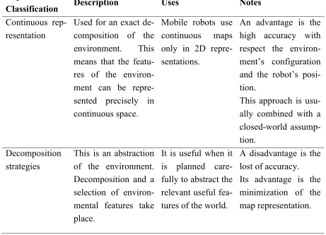
(25) Representation Description Classification Continuous rep- Used for an exact deresentation composition of the environment. This means that the features of the environment can be represented precisely in continuous space.. Decomposition strategies. This is an abstraction of the environment. Decomposition and a selection of environmental features take place.. Uses. Notes. Mobile robots use continuous maps only in 2D representations.. An advantage is the high accuracy with respect the environment’s configuration and the robot’s position. This approach is usually combined with a closed-world assumption. A disadvantage is the lost of accuracy. Its advantage is the minimization of the map representation.. It is useful when it is planned carefully to abstract the relevant useful features of the world.. Table T3.1.1. Environment classification. 3.1 Definition of world map A world map in robotics is the representation of a physical environment in a way that a robot can understand. With this definition, a single environment could be represented in many different ways. Therefore the choice of the map’s definition may be very broad. This leads to the following question: which representation is the best for the robot? To answer it, Roland Siegwart and Illah R. Nourbakhsh recommend in their book “Introduction to Autonomous Mobile Robots” that the following three relationships must be understood first [5]: 1. The precision of the map must appropriately match the precision with which the robot needs to achieve its goals. 2. The precision of the map and the type of features represented must match the precision and data types returned by the robot’s sensors.. 25.

(26) 3. The complexity of the map representation has direct impact on the computational complexity of reasoning about mapping, localization, and navigation. Having these requirements in mind the obvious conclusions is that each representation has an impact on the robot. Table T3.1.1 shows a classification of the environment representation along with current uses, advantages and disadvantages. 3.2 Mapping algorithms fundamentals Once the way to represent the environment has been chosen, the new question to answer is: How does a robot obtain a map? Before answering the question, it is needless to say that creating a map is not an easy task. The readings from the robot’s sensors may contain a lot of noise. In addition, the robot’s motions may not be precise. This can also be seen as noise in the robot’s movements. Many techniques have been developed to overcome this problems and Sebastian Thrun [15] has pointed out that there are already robust methods for mapping static, structured and limited size environments. However, the problem we want to solve is not static at all. Once the robot is in the area it is going to navigate, the environment changes dynamically as there are other agents interacting analogously inside it. Some techniques approach this problem by using short time windows where the environments are considered as static. Thrun also points out that as of today most state-of-the-art robotic mapping algorithms are probabilistic [15], meaning that they use probabilistic models of the environment. The reason behind this lies on what we previously pointed out: robotic mapping is characterized by the noise generated inside and outside the robot’s sensors and the uncertainty produced by them on the robot’s position. 3.2.1. Bayes rule. The Bayes rule is used as the starting point for many statistical mapping algorithms. It relates the chances of the occurrence of event x given the evidence y. It states that:. posterior =. likelihood × prior marginal likelihood. (E3.2.1.1). and is defined by equation (E3.2.1.2). p ( x | y ) = ηp ( y | x ) p ( x ). (E3.2.1.2). 26.

(27) where p(x | y ) is called the posterior probability distribution over X. p(x | y ) specifies the probability of finding y given x. In other words, it makes possible to generate different measures y under different states x. p(x ) is the probability to be at a given state x before any measure, and it is called the prior probability distribution. η is a normalizer used to ensure that it is valid probability distribution. In robotics mapping all data from the sensors is obtained over time. The Bayes filter (see section 3.2.3) is a powerful tool for performing sequential estimations and it is commonly used to integrate this data. 3.2.2. Sequential estimation. To better understand the Bayes filter we point out that a sequential estimation is a method used to estimate a parameter by analyzing large enough data samples until significant results are observed or a certain degree of precision is reached. To further illustrate this concept suppose that the data obtained from one of the robot’s sensor needs to be analyzed. If the probabilistic distribution function of the measurements on that sensor is already known ( p(x ) ), the mean can be obtained directly with:. µ = ∫ xp(x )dx. (E3.2.2.1). In general, p(x ) is not known. Therefore to obtain the mean it is necessary to perform estimations with the data sampled by the sensor. If n samples are obtained {x1 , x2 ,…, xn } the mean can be obtained by equation E3.2.2.2.. m=. 1 n ∑ xi n i=1. (E3.2.2.2). With this approach, all n samples must be known before calculating the mean. However, a better approach is to update the mean as new samples are obtained. For only 1 sample the mean will be m1 = x1 , doing this will also improve the previous estimation of the mean as new samples are acquired. Therefore the mean m in equation (E3.2.2.2) will become a function of the sample xk and the value of the mean before the current sample mk−1 as it shown in (E3.2.2.3):. 27.

(28) mk =. 1 k ∑ xi k i=1. =. 1 1 k−1 x k + ∑ xi k k i=1. =. 1 1 k −1 k−1 xk + ∑ xi k k k −1 i=1. =. 1 k −1 # 1 k−1 & xk + % ∑ xi ( k k $ k −1 i=1 '. =. 1 k −1 xk + mk−1 k k. (E3.2.2.3). This is known as the sequential mean of a random variable [38] and is described by equation (E3.2.2.4).. 1 t −1 mt = xt + mt −1 t t. (E3.2.2.4). where t is the time where the sample is obtained. Posterior probability distribution can also be sequentially estimated as actions are taken and as observations are made [38]. The produced actions and the observed states over time can be modeled and the model can be used to improve the estimates. However we also have to bear in mind that noise will always be present in the observations as in the state, and it has to be included in the model. 3.2.3. Bayes Filter. The Bayes filter is used as a recursive estimator. It consists of two steps. The first one called Prediction update, and the second one called the Measurement update. The Prediction update represents how the current state is expected to be, given the estimate of the previous state and what actions were applied. It is given by equation (E3.2.3.1).. pu(xt ) = ∫ p(xt | xt −1 , at )⋅ mu(xt −1 )dxt −1. (E3.2.3.1). where xt is the current state, xt−1 is the previous state, at is the action taken at time t and the function mu(xt−1 ) is called the Measurement update.. 28.

(29) The Measurement update represents how the observations over time, zt , change the posterior into the prior probability. It comes directly form Bayes rule (E3.2.1.1.1) and is expressed by equation (E3.2.3.2). mu (xt ) = ηp(zt | xt ) pu(xt ). (E3.2.3.2). Where η is a normalizer and pu ( xt ) is the prediction update. By combining equations (E3.2.3.1) and (E3.2.3.2) in a single equation (E3.2.3.3), a generic Bayes filter for simple estimation problems is obtained. With equation (E3.2.3.3) a posterior probability over the state xt can be obtain recursively.. p ( xt | z t ) = η p ( zt | xt ) ∫ p ( xt | xt−1 ) p ( xt−1 | z t−1 )dxt−1 (E3.2.3.3) where z t represents the data obtained from one of the robot’s sensors up to time t, i.e. z t = {z1, z2 ,…, zt }, xt is current state and xt−1 is previous state. As the Bayes filter is recursive, it needs to be initialized with an initial probability at. (. ). time t = 0 . The initial probability is p x0 | z 0 = p(x0 ). In [39] Thrun gives an overview of how p(x0 ) should be initialized when x0 is unknown. The Bayes filter also requires that the state xt contains all unknown quantities that may influence sensor measurements at multiple points in time. In the context of robotic mapping, there are typically two such quantities: the map and the robot’s pose in the environment. Both of them influence sensor measurements over time. Hence, when using probabilistic techniques, the mapping problem is truly one where both the map and the robot pose have to be estimated together [15]. Using m to denote the map and s for the robot’s pose the following Bayes filter is described by equation (E3.2.1.3.4). Notice that s and m comprise the full state vector x, i.e. xt = (st , mt )T. p ( st , mt | z t ) = η p ( zt | st , mt ) ∫∫ p ( st , mt | st−1, mt−1 ) p ( st−1, mt−1 | z t−1 ) dst−1dmt−1. (E3.2.3.4). A detailed discussion about the Bayes rule and the Bayes filter can be found in [39]. 3.2.4. Kalman Filter. Rudolph Emil Kalman introduced the Kalman filter in the1950s. It was primary used as a technique for filtering and predicting in linear systems [39]. Kalman filters are. 29.

(30) (. ). Bayes filters [42] that represent the posterior probability p st , mt | z t with Gausians5. Here we will present a brief description of the Kalman Filter as explained in [15] and [39]. Mapping algorithms based on Kalman filters are often referred to as SLAM algorithms [15]. The mapping relies on the following assumptions: the motion model and the perceptual model must be linear with added Gaussian noise. A linear motion model implies that the pose of the robot and the map at a given time depend linearly on the previous pose and map. However, the Kalman filter is implemented for continuous states. Therefore it is not applicable to discrete or hybrid state spaces. Hence, a modified version was introduced in 1960 called the discrete Kalman Filter. The discrete Kalman filter estimates a process by using a form of feedback control: the filter estimates the process state at some time and then obtains feedback in the form of (noisy) measurements. As such, the equations for the Kalman filter fall into two groups: time update equations and measurement update equations. The time update equations are responsible for projecting forward (in time) the current state and error covariance estimates to obtain the “a priori” estimates for the next time step. The measurement update equations are responsible for the feedback for incorporating new measurements into the a priori estimate to obtain an improved a posteriori estimate. As pointed out previously, the Kalman filter addresses the problem of trying to estimate the state of a discrete-time controlled process governed by a linear model. In cases where a non-linear model is present, the model needs to be approximated by a linear function before using the Kalman filter. Such implementation is referred to as an extended Kalman filter or EKF. 3.2.5. Markov localization. Markov localization is the straightforward application of Bayes filters to the localization problem. It addresses the global localization problem, the position tracking problem, and the kidnapped robot problem in static environments. Markov localization uses an explicitly specified probability distribution across all possible robot positions. The robot's belief6 state is represented as a separate probability assignment for every possible robot pose in the robot’s map. The data from the robot’s sensor measure-. 5. 6. A Gaussian function is a function of the form . The parameter a determines the height of the curve, b is the position of its center, and c determines the width. Gaussians functions are used to describe normal distributions. The robot’s belief about its position on the environment.. 30.

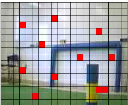
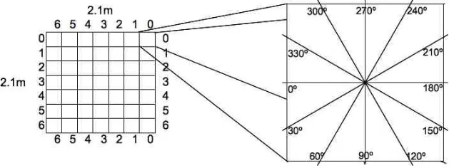
(31) ments is used to update each possible robot position in the belief state individually using the Bayes formula. Therefore, every time a new measure is sensed, the probability of every possible pose of the robot in the map has to be updated as well. A more detailed discussion of these topics is found in [5], [15], [39], [40]. 3.3 Environment set up So far the concept of map in robotics and some of the algorithms that have been used for mapping have been introduced. In this section we will describe how the environment was setup for this work. The environment consisted of an area of 2.1 × 2.1 mts2 divided into 49 square tiles each one of 0.30 × 0.30 mts2, each tile mapped to a Cartesian coordinate in a (x, y ) plane. The following three tasks were performed to set the environment: 1) The landscape was segmented in three coordinates: i. A horizontal coordinate ii. A vertical coordinate iii. An observation angle (x, y, θ ) 2) A picture was taken on each possible (x, y, θ ) coordinate combination i.e. images were taken from 360º around the robot at each coordinate with a 30º step for the observation angle. At each coordinate (x, y ) 12 images were captured (as shown in Figure F3.3.1) yielding a total of 588 images. 3) Each one of the images was digitalized using a standardized RGB format with a total of 640 × 480 pixels per image. 4) Each one of the images was manipulated in GIMP to resize them using the Sinc (Lanczos 3) interpolation [37] to a resolution of 176 × 144 pixels. All images were saved in the PPM format (Portable Pixel Map [9]), which maintains constant file size for all images. To reduce the amount of rough data the images were then sampled at regular interval every 16 pixels by our algorithm. These images formed a database that included information about the position of the image. This information consists of the x, y coordinates and the angle θ of the image. All of these images will be used as offline training data so the robot can know its position by looking only into the database for an image that match with what its sensor is getting at some future time. It is true that there may be cases where some ambiguity will occur. For example, when the robot is to close to a wall and it is facing to it. 31.

(32) or it is to close to a post or simply by looking directly to the floor. In those circumstances, a possible solution is to make the robot turn its head and camera to a different angle to take a new picture.. Fig. F3.3.1.. 3.3.1. Illustration of the sampled area.. The Portable Pixel Map Format. The PPM format is a color image file format that can contain one or multiple images in a single ppm file that can be ASCII or binary. In the file there are no data delimiters or padding before, after, or between images. The file consists of two parts. In the first part lies the general description of the file. Among other things, the first part of the file contains the type of the file, the height and width of the images and the maximum color value. The second part of the file is a raster that represents one or multiple images, every width pixels in the raster represents a row of the image and the raster will have height number of rows in it to represent a single image. Each pixel in the row is the value of the red, green, and blue samples of the pixel in this order. Each sample can be either 1 or 2 bytes of size depending on the maximum value reported in the first part of the file. For this work, a binary representation of the file was used, leading to 54 bytes (from byte 0x0000 to 0x0035) that represent the description of the file. The second part, starts from byte 55 (0x0036 onwards) and it is a raster that represents the images. As we used images of size 176 × 144 pixels, every 528 bytes in the raster represented a row of pixels of the image in the RGB color space. The reason behind using this format is that it is easier to process the pixel information as they all had the same amount of information.. 32.

(33) 3.3.2. Data set up. As pointed in the previous section, in th PPM format, each pixel value in the raster that represent the image is composed by 3 bytes, one byte for color red, gree and blue. Therefore, the total amount of bytes in only one picture of size 176 × 144 pixels is 76,032 ((176 × 3) × 144), hence the total amount of pixels in the database for the 588 images is 44,706,816 (76,032 × 588). This simple exercise gives an idea of the huge amount of information that needs to be processed and the implication on the time need to perform the computations. In order to further reduce the amount of data, a pixel out of 16 was selected leaving with only 1,584 pixels per image to work with. The database of images was created reading each of the PPM images files, discarding all the information using only the information of the pixels values. 4. Determination of the Sieve. The method consists of the extraction of a fixed number of pixels from an image captured by the robot along with their position (in the image) to perform a search in a database that will contain all images loaded into the robot’s memory. With this set of pixels, a single image must be identified from all the images in the set, and the amount of pixels in the set must have to be the minimum. In figure F4.1 we illustrate an image and its possible representations by two different sieves. The main motivations to reduce the amount of information in the database are that it must fit into the robot’s memory and that this information is to be processed in real time. The first issue is vital if there are limited resources of memory space and processing power in the robot. At first glance, to overcome this problem the robot’s memory can be increased as well as its processing power, but there is a better choice. The database size may be reduced in a way that it only holds a minimum amount of data required to identify an image. To achieve the reduction in size, a number of pixels p, expected to be less than the total number of pixels that conforms an image (i.e. 1,584 in this case) must be found. Additionally the number of pixels p should be such that an image should not be wrongly identified. It is obvious that if the number of selected pixels in the sieve reaches the total number of pixels in the image, the probability to identify an image as a different one will be low. On the other hand, if the number of pixels is minimum, e.g. one pixel, the probability to misidentify an image in the database will be high. Therefore, two things have to be minimized: a) The number of pixels p in the sieve required to identify an image, 33.

(34) b) The image identification error, ε I .. Fig. F4.1. An image of the environment and its possible representation by a set of pixels. 34.

(35) This is a typical multi-objective optimization problem with conflicting goals. In section 2.2 we mentioned that there are different ways to approach these kinds of problems, e.g., by aggregating the objectives into a single objective function. A different approach is by using a Multi-Objective Evolutionary Algorithm (MOEA).. Fig. F4.2. A sample view of 10 individuals for images of 35 pixels. The algorithm we propose uses a population of n individuals. Each individual genome is the size of the number of pixels in the image, i.e. 1,584. Every allele in the genome maps directly to a position of a pixel in the image. The set of alleles with a value of 1 represent the pixels that will work as a sieve, which will be used to select the pixels of all the images in the same position. In other words a bit turned on in the genome means that the pixel in that position will be part of the sieve. The number of pixels that will be part of the sieve is selected randomly. Figure F4.2 shows a set of 10 individuals created for hypothetical images of 35 pixels each one. Every dark rectangle in the image represents the position of the pixel selected to be part of the sieve. Each individual may have a similar or different sieve sizes as it is also shown in the figure. To evaluate the candidate sieve, a random image is selected from the set of images. The pixels in the sieve are then compared with the remaining images. Every time that the value of a pixel is in another image, a counter for the candidate sieve is increased. This counter will provide the number of repetitions found across all the images. The number of repetitions is called the pixel identification error, ε . The number of pixels repeated per image is called the image identification error, ε I . To find ε I , the pixel identification error ε is divided by the total number of images (588) and the number of pixels that form the sieve. The result is then multiplied by the number of pixels that correspond to a single image as shown in equation (E4.1).. εI =. ε Ti s. N. (E4.1). 35.

(36) where: ε I is the image identification error, ε is pixel identification error, Ti is the number of images, s are the pixels in the sieve and N is the number of pixels in an image. The population in the MOEA will produce a set of points that will be part of the solution space. If there is a subset of points in the solution space that dominates all the other solutions, then this subset will outline a Pareto front. This process is repeated each generation. If the number of pixels in the sieve falls in a predefined threshold, the algorithm has reached the optimal set of points in the sieve, which allow us to satisfy objectives a) minimize the size of the sieve s and b) minimize ε I . 4.1 Adjustments performed to the RPSGAe algorithm The MOEA used to solve this problem was the RPSGAe algorithm implemented in Java and introduced in section 2.2.5.3. Several runs were performed and the algorithm took more than 40 minutes to find a Pareto front. A closer analysis of the implementation revealed that the clustering procedure was consuming most of the processing time. As there were only two objective needed to be optimized, it was decided that the clustering module was unnecessary and therefore it was eliminated from the implementation. This simple modification speeded up the processing time to just a few minutes. It is important to point out that the RPSGAe algorithm leaves open the implementation of the genetic operators: selection, crossover and mutation. Therefore the genetic operators were implemented as in the Eclectic Genetic Algorithm [31] to include: Deterministic Coupling, Full Elitism and Annular Crossover. By doing so we can take advantage of a high degree of elitism and at the same time give variety to the genetic pool [31]. 5. Obstacles in the field of view. With this method, the robot expects to find a perfect landscape in the sense that it ought to unequivocally determine at least one of the identifying sieves. There are two possible reasons for which an image may not be identified: a) There is too much noise in the image or b) There is an object (originally not present) which is obstructing the field of view of the robot. When this does occur, it must be that something happening in its environment modified the landscape in its field of view. In this hypothetical case, (and discarding the possibility of excessive noise in the environment) one must conclude that a new object (not present in the original scenery) is causing. 36.

(37) the ambiguity of position problem. In our case, rather than becoming a nuisance, this fact will allow us to a) Determine the presence of an extraneous object and b) Determine the precise nature of such object. If we assume a finite collection of extraneous objects we will be able to characterize them much the same way we were able to characterize the environment. Following this line of reasoning, we can introduce new data to determine what caused the change in the landscape and where this change occurred. 5.1 Enemy identification Once the problem of identifying the robot’s position has been dealt with, there is a second possible application of the method. Namely, it does allow us to take one-step further and identify the strange objects in the field of view. In the context of a soccer match such as the ones in RoboCup, the possible obstructions (and the consequent inability to identify an image from its sieve) must be due to the presence of an alien object not present in the course of image acquisition. These objects are hereinafter called “enemies”. To be able to identify an enemy it is necessary to take pictures of each enemy to create a new set of images that will form an enemy database. Then we can identify them by applying morphologic operators, which make such enemy images position and scale independent. At that point, the non-identification of a robot’s position is an advantage. Since it implies the detection of the presence of an undesirable (in the sense that a robot playing soccer must avoid it) obstacle. Furthermore, it allows the robot to identify the type and distance of the enemy relative to the present position. It is important to clarify that the enemy identification was not done as part of the present work; it was included here only as an example of a different application that the sieve method may have. 6. Validation of the sieve. To demonstrate the effectiveness of the Optimum Sieve method proposed in this work a statistical validation method was performed using two similarity measures: 1. The Hamming distance 2. The Euclidean distance This section describes the similarity measures and the data used in the validation.. 37.

(38) 6.1 Data setup for the validation To validate this method a new database of images was set up. The validation method applied to this database used both: a) The complete set of pixels (1,584) and b) The reduced set of pixels found by the MOEA. The new database was setup by 28 images acquired from a unique point located in the center of the area showed in figure F3.4.1. The images have a separation of 5 degrees between them and sweep a range from zero to 30 degrees in the horizontal and from zero to 20 degrees in the vertical as oppose to the original set of images that had a separation of 30 degrees between them only in the horizontal. The robot’s camera was facing forward and parallel to the ground. 6.2 Similarity measures Given the nature of the problem there should be a way that can help determine if an image the robot is sensing at a specific time is similar to another image in the robot’s database. If the two images are alike, then the probability that the robot is in the same position as the image in the database is high, and it will be low if the two images are different. Therefore, the robot is set in a different position. To be able to measure how different is an image from another a similarity measure between images is needed. In the present work, two different measures were used. One was the Hamming distance (between two sets of pixels). The other was the Euclidean (which determines how "far" or “similar” are the components of a pixel relative to another one). 6.2.1. Minkowski metric. Given two points x = (x1 , x2 ) and y = ( y1 , y2 ) , a general measure of their closeness is the p-Minkowski [11] metric given by. d. p. (x, y ) = [x1 − y1. p. + x2 − y2. 1 p p. ]. (E6.2.1.1). where p is a positive real number such that p ≥ 1. For p=1, d (x, y ) is the Hamming distance. For p=2, d 2 (x, y ) is the well known Euclidean distance. For p= ∞ equation (E6.2.1.1) reduces to. d ∞ (x, y ) = max[ x1 − y1 , x2 − y2 ] 38. (E.6.2.1.2).