Applications of hydrodynamic and water quality models to the Sau and Boadella Reservoirs

Texto completo

(1)APPLICATIONS OF HYDRODYNAMIC AND WATER QUALITY MODELS TO THE SAU AND BOADELLA RESERVOIRS Saddek TAKKOUK. ISBN: 978-84-694-5169-4 Dipòsit legal: GI-772-2011 http://hdl.handle.net/10803/31853. ADVERTIMENT. La consulta d’aquesta tesi queda condicionada a l’acceptació de les següents condicions d'ús: La difusió d’aquesta tesi per mitjà del servei TDX ha estat autoritzada pels titulars dels drets de propietat intel·lectual únicament per a usos privats emmarcats en activitats d’investigació i docència. No s’autoritza la seva reproducció amb finalitats de lucre ni la seva difusió i posada a disposició des d’un lloc aliè al servei TDX. No s’autoritza la presentació del seu contingut en una finestra o marc aliè a TDX (framing). Aquesta reserva de drets afecta tant al resum de presentació de la tesi com als seus continguts. En la utilització o cita de parts de la tesi és obligat indicar el nom de la persona autora. ADVERTENCIA. La consulta de esta tesis queda condicionada a la aceptación de las siguientes condiciones de uso: La difusión de esta tesis por medio del servicio TDR ha sido autorizada por los titulares de los derechos de propiedad intelectual únicamente para usos privados enmarcados en actividades de investigación y docencia. No se autoriza su reproducción con finalidades de lucro ni su difusión y puesta a disposición desde un sitio ajeno al servicio TDR. No se autoriza la presentación de su contenido en una ventana o marco ajeno a TDR (framing). Esta reserva de derechos afecta tanto al resumen de presentación de la tesis como a sus contenidos. En la utilización o cita de partes de la tesis es obligado indicar el nombre de la persona autora. WARNING. On having consulted this thesis you’re accepting the following use conditions: Spreading this thesis by the TDX service has been authorized by the titular of the intellectual property rights only for private uses placed in investigation and teaching activities. Reproduction with lucrative aims is not authorized neither its spreading and availability from a site foreign to the TDX service. Introducing its content in a window or frame foreign to the TDX service is not authorized (framing). This rights affect to the presentation summary of the thesis as well as to its contents. In the using or citation of parts of the thesis it’s obliged to indicate the name of the author..

(2) Application of a hydrodynamic and water qaulity models to the Sau and Boadella Reservoirs. Saddek Takkouk. Thesis work supervised by Xavier Casamitjana Vila. January 2011.

(3) Acknowledgments This work was supported by the former International Graduate School of Catalonia of the Government of Catalonia (IGSOC). First of all, I would like to thank my supervisor, Xavier Casamitjana, for providing me with this opportunity and for his guidance along the way. Likewise, thanks to the Environmental Physics group members, Jordi Colomer, Teresa Serra and Marianna Soler. I would like to thank Jörg Imberger for providing me with the model (CWR DYRESMCAEDYM) and also Jason Antenucci for teaching me the online DYRESM-CAEDYM course. My thanks also go to Joan Armengol of the Ecology Department of Barcelona University for providing me with Sau Reservoir data and to the Meteorologic Service of Catalonia and the Catalan Water Agency, represented by Carlos Baserba, for providing me with Boadella Reservoir data. Also, I would like to thank the entire staff of the Physics Department for contributing to and helping me complete this thesis, especially Elena Roget, Josep Calbo, Josep González, Xisco, Eduard and Toni. In addition, I would like to thank my wife, for her unwavering support, and my children, Mohamed Abdel Mouiz, Anfel, Afnane and Alaa Ayat Errahmane. També vull donar les gràcies a la Universitat de Girona per haver-me acceptat en el Programa de doctorat, i a la Generalitat de Catalunya per donar-me aquesta oportunitat de finançament de l’estudi. Finalment, vull donar les gràcies a tots els catalans de la UdG, a l’associació de pares i mares de l’Escola Cassià Costal i al Grup Excursionista i Esportiu Gironí (GEiEG).. i.

(4) INDEX Index. ii. Acknowledgements. i. Summary. 3. Chapter 1: “Introduction”. 3. 1.1 General frame 1.2 Study site 1.2.1 Sau Reservoir 1.2.2 Boadella Reservoir 1.3 Seasonal Thermal Structure 1.4 Inflows and Outflows 1.4.1 Inflows 1.4.2 Outflows 1.5 Lake regime classifications 1.6 Objectives 1.7 Methods 1.7.1 DYRESM description 1.7.2 CAEDYM description. 3 7 7 10 12 13 13 14 16 17 19 19 25. Chapter 2: “Data Analysis and Field Experiments”. 36. 2.1 Introduction 2.2 Study Sites. 36 36 36 37 38 40 40 42 42 42 44 44 45 46 48 48. 2.2.1 Sau reservoir 2.2.2 Boadella Reservoir 2.3. Data introduction 2.4 Sau Reservoir data 2.4.1 Morphometric Data 2.4.2 Meteorological data 2.4.2.1 Air temperature 2.4.2.2 Solar radiation (short wave and long wave radiation) 2.4.2.3 Vapour pressure 2.4.2.4 Wind velocity 2.4.2.5 Precipitation 2.4.3 Inflow 2.4.4 Outflow 2.4.5 Sau reservoir Profiles. ii.

(5) 2.4.5.1 Temperature Profiles 2.4.5.2 Dissolved Oxygen profiles 2.4.5.3 Phosphorous 2.4.5.4 Chlorophyll 2.5 Boadella Reservoir Data 2.5.1 Morphometric Data 2.5.2 Meteorological data 2.5.2.1 Air temperature 2.5.2.2 Solar radiation 2.5.2.3 Vapour pressure 2.5.2.4 Wind velocity 2.5.2.5 Precipitation 2.5.3 Inflow 2.5.4 Outflow 2.5.5 Boadella reservoir Profiles 2.5.5.1 Temperature Profiles 2.5.5.2 Dissolved Oxygen Profiles 2.5.5.3 Phosphorous 2.5.5.4 Chlorophyll. 48 49 50 51 52 52 53 53 54 56 56 57 58 60 60 60 61 62 63. Chapter 3: “Criteria for using a one-dimensional DYRESM model. 64. in the Sau and Boadella reservoirs” 3.1 Introduction 3.2 Lake Number 3.3 Wedderburn Number 3.4 Burger Number 3.5 Inflow Froude Number 3.6 Outflow Froude Number 3.7 Methods 3.8 Results and discussions 3.8.1 Lake number 3.8.2 Weddeburn number 3.8.3 Burger number 3.8.4 Inflow Froude number 3.8.5 Outflow Froude number 3.9 Conclusions. 64 65 66 67 68 69 69 71 71 73 74 75 76 77. Chapter 4: “Application of the Dyresm-Caedym model. 78. to the Sau Reservoir” Abstract 4.1 Introduction. 78 78. iii.

(6) 4.2 Materials and Methods 4.3 DYRESM-CAEDYM model 4.4 DYERESM-CAEDYM Calibration and Validation 4.5 Simulation and results 4.6 Conclusion. 79 80 84 90 104. Chapter 5: “Application of the Dyresm-Caedym model. 106. to the Boadella Reservoir” Abstract 5.1 Introduction 5.2 Materials and Methods 5.3 DYRESM-CAEDYM model 5.4 DYERESM-CAEDYM Calibration and Validation 5.5 Simulation and results 5.6 Conclusion. 106 106 108 110 111 116 127. General Conclusions. 130. References. 134. iv.

(7) Figure list. Pages. Figure 1.1. Bathymetric map of the Sau Reservoir.. 9. Figure 1.2. Boadella Reservoir bathymetry.. 11. Figure 1.3. Schematic representation of mixing processes in a lake. Taken from Imboden and Wüest (1995).. 13. Figure 1.4. Inflow dynamics.. 14. Figure 1.5. Evolution of the outflow from the opening of the outlet to the generation of the jet flow. Blue lines represent isopycnals.. 15. Stratification process due to the water withdrawal from a selective outlet. The blue line indicates the temperature profile evolution and the shadowed area indicates the sink line.. 15. Figure 1.7. Summary of the biogeochemical paths simulated in CAEDYM.. 26. Figure 1.8. Simplified schematic of the DO Dynamic within CAEDYM.. 28. Figure 1.9. Generic schema of the nutrient dynamics with CAEDYM.. 29. Figure 1.10. Phytoplankton dynamics within CAEDYM.. 30. Figure 2.1. Sau Reservoir bathymetry.. 37. Figure 2.2. Boadella Reservoir bathymetry.. 38. Figure 2.3. Sau Reservoir Area-Elevation.. 41. Figure 2.4. Sau Reservoir Volume-Elevation.. 41. Figure 2.5. Daily air temperatures in the Sau Reservoir.. 42. Figure 2.6. Sau Reservoir time series of short wave radiation (A) and long wave radiation (B).. 43. Figure 2.7. Sau Reservoir time series of vapour pressure.. 44. Figure 2.8. Sau Reservoir daily wind velocity.. 45. Figure 2.9. Sau Reservoir daily rainfall and accumulated rainfall.. 46. Figure 2.10. Daily inflow temperature (A); Daily inflow volume entering the Sau Reservoir (B).. 47. Figure 1.6. v.

(8) Figure 2.11. Daily outflow volume.. 48. Figure 2.12. Field temperature time series.. 49. Figure 2.13. Sau Reservoir time series of Observed Dissolved Oxygen.. 50. Figure 2.14. Daily Dissolved inorganic phosphorous in the Sau Reservoir.. 51. Figure 2.15. Sau Reservoir chlorophyll time series. 51. Figure 2.16. Boadella Reservoir Area-Elevation.. 52. Figure 2.17. Boadella Reservoir Volume-Elevation.. 53. Figure 2.18. Boadella Reservoir air temperature time series.. 54. Figure 2.19. Short-wave radiation (A) and cloud cover (B) time series.. 55. Figure 2.20. Boadella Reservoir vapour pressure time series.. 56. Figure 2.21. Boadella Reservoir wind speed time series.. 57. Figure 2.22. Daily and accumulated rainfall for the Boadella Reservoir.. 58. Figure 2.23. Boadella Reservoir daily inflow temperatures (A) and daily inflow volume (B).. 59. Figure 2.24. Boadella Reservoir outflow time series.. 60. Figure 2.25. Boadella Reservoir time series of observed temperature.. 61. Figure 2.26. Boadella Reservoir time series of measured dissolved oxygen.. 62. Figure 2.27. Boadella Reservoir time series of field dissolved inorganic phosphorus.. 62. Figure 2.28. Boadella Reservoir chlorophyll time series.. 63. Figure 3.1. The differences in the Sau and Boadella Lake numbers.. 72. Figure 3.2. Sau and Boadella Wedderburn numbers.. 73. Figure 3.3. Comparison between the Sau and Boadella Burger numbers. Sau is represented by squares, and Boadella by circles.. 74. Sau and Boadella inflow Froude numbers.. 75. Figure 3.4. vi.

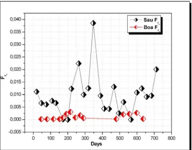
(9) Figure 3.5. Sau and Boadella outflow Froude numbers.. 76. Figure 4.1. Bathymetric map of the Sau Reservoir showing the location of measuring stations and the meteorological station.. 80. Figure 4.2. The coupled DYRESM-CAEDYM model simulates temperature, dissolved oxygen, phosphorus and chlorophyll in the Sau Reservoir. 83. Figure 4.3. Figure 4.4 Figure 4.5. Figure 4.6 Figure 4.7 Figure 4.8 Figure 4.9 Figure 4.10 Figure 4.11 Figure 4.12. vii. Average absolute difference standard error of the mean between DYRESM-CAEDYM predicted and observed water temperature (white), bottom water temperature (gray) and thermocline depth (line) at various layer thickness setting (A), wind stirring efficiency values (B), Vertical mixing coefficient (C), effective surface area coefficient (D), albedo and potential energy mixing coefficient values (E), and base extinction coefficient(F).. 87. One year (2001): Simulated temperature (A), Measured temperature (B) and Comparison (C).. 94. Comparison of temperature profiles between observed and simulated results on four Julian days: 44, 101,199 and 290 of the year2001. Squares represent the observed results and the lines represent the simulations.. 95. One year (2001): Simulated dissolved oxygen (A), Measured dissolved oxygen (B) and Comparison (C).. 96. One year (2001): Simulated dissolved inorganic phosphorus (A), Measured dissolved inorganic phosphorus (B) and Comparison (C).. 97. One year (2001): Simulated chlorophyll (A), Field chlorophyll (B) and Comparison (C).. 98. Two years (2000-2001): Simulated temperature (A), Measured temperature (B) and Comparison (C).. 99. Two years (2000-2001): Simulated dissolved oxygen (A), Measured dissolved oxygen (B) and Comparison (C).. 100. Two years (2000-2001) Simulated dissolved inorganic phosphorus (A), Field dissolved inorganic phosphorus (B) and Comparison (C).. 101. Two years (2000-2001): Simulated Chlorophyll (A), Field Chlorophyll (B) and Difference.. 102.

(10) Figure 4.13. Comparison between water surface simulation (open circles) and observation (filled circles) of Temperature (A), Dissolved oxygen (B), Phosphorus (C) and Chlorophyll (D).. 104. Figure 5.1. Boadella Reservoir bathymetry.. 109. Figure 5.2. Average absolute difference standard error of the mean between DYRESM-CAEDYM predicted and observed water temperature (white), bottom water temperature (gray) and thermocline depth (line) at various layer thickness setting (A), wind stirring efficiency values (B), Vertical mixing coefficient (C), effective surface area coefficient (D), albedo and potential energy mixing coefficient values (E), and base extinction coefficient(F).. 113. One year (2000) of temperature values: simulated (A), measured (B) and comparison (C).. 119. Comparison of temperature profiles between observed and simulated results on Julian days 46, 117, 192 and 272 of the year 2000 (dashed line: observation, solid line: simulation).. 120. One year (2000) of dissolved oxygen values: simulated (A), measured (B) and comparison (C).. 121. One year (2000) of chlorophyll values: simulated (A), measured (B) and a comparison (C).. 122. Two years (2000-2001) of simulated temperatures (A), measured temperatures (B) and a comparison (C).. 123. Two years (2000-2001) of simulated DO (A), measured DO (B) and a comparison (C).. 124. Two years (2000-2001) of simulated chlorophyll (A), measured chlorophyll (B) and a comparison (C).. 125. Comparison between water surface simulation (open circles) and observation (filled circles) of temperature (A), dissolved oxygen (B) and chlorophyll (C).. 127. Figure 5.3 Figure 5.4. Figure 5.5. Figure 5.6 Figure 5.7 Figure 5.8 Figure 5.9 Figure 5.10. viii.

(11) Table list. Pages. Table 1.1. Summary of the governing equations in DYRESM. 20. Table 1.2. List of Hydrodynamic symbols. 21. Table 1.3. Main equations used in CAEDYM for the biogeochemical paths. 32. Table 1.4. list of symbols and variables. 34. Table 2.1. Morphometric characteristics of the Sau Reservoir. 40. Table 4.1. Values of coupled model parameters and model simulation specifications.. 86. The major calibrated water quality parameters used in the DYRESMCAEDYM model.. 89. Values of coupled model parameters and model simulation specifications.. 112. Calibrated water quality parameters used in the DYRESMCAEDYM model.. 115. Table 4.2 Table 5.1 Table 5.2. ix.

(12) x.

(13) SUMMARY Density stratification is crucial for the hydrodynamics as well as for the ecosystems functioning in almost all lakes. Most important for stratification is the temperature dependence of the water density. Stratification might change due to the meteorological effects, inflow and outflow producing the so-called ecological response of the reservoir. In recent years many physical limnology studies have been carried out in many reservoirs in the world; most of them are specifically related to water quality issues. This PhD thesis therefore, aims to highlight an assessment of the main physical mechanisms of two medium-sized reservoirs situated in Catalonia. The focus is on the Sau and Boadella reservoirs located in Catalonia, in northeast Spain, but some of the results obtained here can be extended to other medium-sized reservoirs situated in the same region and climate. The Sau and Boadella reservoirs are both quite eutrophic in nature and supply drinking water to the area of Barcelona and Girona (Figueres). Therefore, having a better understanding of the main physical processes and the ecological response of the reservoir to such processes might be of significant help to the water management authority. We intend to use a 1D hydrodynamic model linked with water quality (DYRESMCAEDYM) if the conditions of application of such model which will be checked in chapter three are met. In order to characterize the dynamical regimes for the Sau and Boadella reservoirs, it is important to estimate the Wedderburn number, the Lake number, the Burger number and the inflow/outflow Froude numbers. the Wedderburn number is an indicator of the upwelling of metalimnetic water, the Lake number is an indicator of upwelling of hypolimnetic water, the Burger number characterizes the influence of the earth’s rotation on the water movement in reservoirs and the inflow/outflow Froude numbers are related to the river when it enters the reservoirs and water that flows out of the reservoirs.. 1.

(14) Summary Sau is a canyon type reservoir, with only one tributary, the Ter River, while the Boadella has two tributaries, the Arnera and the Muga rivers. It should be mentioned that the Boadella Reservoir is used for comparison purposes. For both reservoirs, there were two years (2000-2001) available input data for the DYRESM-CAEDYM model. Simulated parameters are temperature, dissolved oxygen, dissolved inorganic phosphorus and chlorophyll. However, significant unknown river data are daily dissolved oxygen, nutrients and chlorophyll. We therefore suggest a hypothesis based on the available reservoir water quality profiles. For every month’s water quality profile we take the mean concentrations of each of them and use the most repeated one as the daily river concentration input over the simulation period. The DYRESM-CAEDYM model needs to be calibrated to get simulated values well adjusted to observed ones. The calibration process is the most difficult task due to time consuming and the large number of hydrodynamic and water quality parameters to be calibrated. For both reservoirs, the calibration process was done by trial-and-error adjustment of the most sensitive parameters in different calibration periods. The calibration process has to be done in this order: temperature, dissolved oxygen, phosphorus and chlorophyll. The last one, however, is the most difficult to calibrate because it depends on the previous calibrated parameters. Therefore, errors in the calibration process have to be accepted. During the spring-summer season of 2000 and 2001 the Sau Reservoir stratifies and a thick metalimnion is formed. DYRESM-CAEDYM simulates temperature stratification very well. For dissolved oxygen the model gives a good simulation, indicating an anoxic zone at the bottom during the stratification period. Also, simulated soluble inorganic phosphorus has the same trend as in the field. Nevertheless, the measured inorganic phosphorus is much higher, and the reason might be the loading discharge of the phosphorus source at the bottom of reservoir, or it could be the river inflow. Even with calibration, chlorophyll simulation is the most difficult task to achieve. The simulated chlorophyll is far from the measured value in the mixed surface layer. This can be due to the fact that some phytoplankton species were not taken into consideration or to the limitation of a one dimensional model.. 2.

(15) Summary Meanwhile, for Boadella Reservoir the modelling exercise, for the same simulation length 2000-2001, shows that for the temperature stratification period (from spring-summer) and overturn period (through the autumn and winter), the simulated dissolved oxygen is quite similar to that predicted in the Sau Reservoir. Unfortunately, in the Boadella Reservoir there was a lack of observed data of phosphorus to comparing it with the simulated one. But simulated chlorophyll is better than in the Sau Reservoir. In general, DYRESM-CAEDYM is a good water quality management tool since it can make accurate predictions of temperature, dissolved oxygen, and, with less confidence, phosphorus and chlorophyll.. 3.

(16) Summary. 4.

(17) Introduction. CHAPTER 1 Introduction 1. 1 GENERAL FRAME. The eutrophication of lakes and reservoirs attributable to increase of nutrients loading particularly of nitrogen and phosphorus that can be increased algal bloom formation, which is a major water quality issue worldwide. Eutrophication is the naturally occurring process by which water bodies become more productive, changing from oligotrophic (low nutrient supply) to eutrophic (rich in nutrients) (Bayly & William 1973). This nutrient enrichment is coupled with an increase in phytoplankton growth. The most important factors controlling the growth are availability of nutrients, light and mixing conditions. Excessive abundance of phytoplankton generally has detrimental effects on the domestic, industrial and recreational uses of water bodies. During periods of algal blooms oxygen depletion occurs in the lower water column, often resulting in fish kills. Furthermore, as the algae grow and decompose, aesthetic and odour problems arise, due to the accumulation of scum on the water surface and shores (Soranno 1997). Potentially, toxic phytoplankton can be a serious health risk to humans and animals, and have been implicated with numerous poisoning incidents worldwide (Carmichael et al. 2001). Therefore, in recent years, the study of the motion and mixing of water in lakes and reservoirs has been developed. Water hydrodynamics in these reservoirs are generated in response to surface wind stress, rotational effects, river inflow or outflow, and differential heating. The sophisticated machines with large processors made easier for us to run complex hydrodynamic models coupled with water quality models. The hydrodynamics in aquatic systems is connected with vertical stratification, that could be enhanced or weakened by chemical constituents, and depends on the interplay between the dominant disturbance forces, which are mechanisms energizing the water motion, and the restoring forces such as potential energy, sometimes the earth’s rotation, and reservoir bathymetry. 5.

(18) Chapter 1 It is very important to understand the hydrodynamic of a reservoir because mixing and transport processes are of greatest importance to water chemistry and biology in reservoirs which reveals the ecological response of the reservoir to meteorological forcing, inflows and outflows (Imberger 1998) and (Imberger 1994, Imberger 1990, Fischer et al. 1979). For this reason, evaluating aquatic management strategies for lakes and reservoirs is necessary. Several hydrodynamical and water quality models have been developed to study the seasonal dynamics amid these model, a simple empirical models that have been developed since the mid-1960's to predict eutrophication on the basis of the phosphorous (P) loading concept (Vollenweider, 1968) (see reviews by Mueller, 1982, and Ahlgren et al., 1988). Afterward, several models have been developed following this approach. Examples include AQUASYM (Reichert, 1994), GIRL (Kmet and Straskraba, 1989) and MONOD (Karagounis et al., 1993). Finally, an approach that has been developed for 1D hydrodynamic model to include water quality parameters such as DLM-WQ , CEQUAL-R1 (USCE, 1995), MINILAKE (Riley and Stefan, 1988), DYRESMWQ (Hamilton and Schladow, 1997), and (CE-QUALR1, MINILAKE, DYRESM-WQ, and 1-D, 3-D Dynamic Reservoir Simulation Model DYRESM, ELCOM coupled with ecological model CAEDYM these last two models were developed in the water center of the western university of Australia.. Our focus is on the one dimensional. hydrodynamic model DYRESM coupled with ecological model CAEDYM which is worldwide used model especially for lakes and reservoirs. Therefore, DYRESM model has been applied for Sau reservoir by (Vidal et Om. 1993), (Armengol. et al. 1994 and 2003) and (Han et al 2000) who have studied the effect of river on the longitudinal process and thermal structure in Sau reservoir. (Casamitjana. et al. 2003) used another hydrodynamic model (DLM) to study the effect of withdrawal in Boadella reservoir. (Andrew. et al. 2007) have used calibrated DYRESM to simulate boreal lake. (Louise. et al. 2006) have used DYRESM-CAEDYM to simulate seasonal dynamics of nutrient in Lake Kinneret. Also (Romero. et al. 2004) have applied DYRESM-CAEDYM and ELCOM-CAEDYM to simulate underflow through Lake Barrgorang. (Schladow et al. 1997) have employed DYRESM-CAEDYM to predict water quality in lakes and Reservoirs in part I and II. (Hmilton. et al. 1995) have applied (DYRESM-CAEDYM) 6.

(19) Introduction model to control the indirect effect on water quality in an Australian Reservoir. (Antenucci. et al. 2003) have examined DYRESM-CAEDYM to study the effect of artificial destratification in management strategies for a eutrophic water supply reservoir San Roque, Argentina The present study focuses on the criteria of using such one dimensional hydrodynamic model DYRESM linked to water quality model CAEDYM. if, this criteria was checked Then could be applied to Sau and Boadella reservoirs. The major goal is to contribute to a better understanding of the main physical-ecological processes interaction and the water quality consequences affecting both of these reservoirs. Therefore, DYRESMCAEDYM model was used to simulate water temperature, dissolved oxygen, phosphorus and chlorophyll. 1.2 STUDY SITE 1.2.1 Sau Reservoir The Sau Reservoir was selected as the main study site and the focus of this PhD for three reasons: first, it is a good representative example of Spanish and Mediterranean reservoirs; second, it has been widely studied since it was first filled in 1964; and last, it is one of the chain of reservoirs reservoir supplying water to the capital of Catalonia. In Chapter 5 I will also study the Boadella Reservoir, which is smaler than the Sau Reservoir. Sau is an eutrophic reservoir with incoming nutrients from the River Ter, polluted due to human activity in the watershed (Vidal and Om 1993, Armengol et al. 1994). Its eutrophication process and evolution since it was first filled have been described by Vidal (1977). River valley reservoirs, such as the Sau Reservoir, are often large and narrow, and only receive water from a single river inflow. These reservoirs have important longitudinal changes controlled by the river intrusions across them (Hejzlar & Straškraba, 1989). Thus these reservoirs could be considered as hybrid systems between inflowing rivers and lakes (Margalef, 1983), with a progressive transformation from a river to a lake system, not only in terms of environmental variables, but also in their morphology and hydrodynamic characteristics. In general, a reservoir can be divided 7.

(20) Chapter 1 along the longitudinal axis into three zones (Kimmel et al., 1990): the riverine zone, where it characterised by relatively high flow velocity; the transition zone, with moderate flow velocity; and the lacustrine zone, where the water is stagnant and the flow velocity is negligible. The riverine zone is characterized by a higher flow and consequently high Froude numbers, which is the report of inertia and gravity, short residence time and high values of nutrients and suspended solids. The transition zone, where the river meets the reservoir, is characterized by moderate velocity, moderate Froude and dissymmetric Froude numbers, high phytoplankton productivity and relatively large sedimentation. Finally, the lacustrine zone, consisting of the area near the dam, is characterised by low Froude numbers and considerable dissymmetric Froude numbers corresponding to long residence time, lower available nutrients and lower suspended matter. In response to inflow characteristics, the canyon-type morphology of the Sau Reservoir (Fig. 1.1) results in a marked longitudinal heterogeneity in the community populations (Armengol et al. 1999, Comerma 2003) and also affects the hydrodynamics. The main body of the reservoir, where the dam is located, corresponds roughly to the lacustrine zone; this zone behaves like a lake because the wind is the main forcing mechanism influencing the hydrodynamics. However the riverine and transition zones are narrow and meandering and sheltered from the wind forcing. The hydrodynamics in these zones is mainly affected by the river inflow. Of course, no strict boundaries between the zones exist and the hydrodynamics generated in one zone can affect the rest of the reservoir. Nevertheless, separating the reservoir into these zones will be useful in studying the main processes taking place in each one.. 8.

(21) Introduction. Figure 1.1 Bathymetric map of the Sau Reservoir. 9.

(22) Chapter 1 1.2.2 Boadella Reservoir The Boadella Reservoir is located in the north-east of Spain in the eastern prepyrenees was built in response to urban growth, tourist development, intensive agriculture and the demand for drinking water is relatively small compared to Sau Reservoir. However, this last was selected in this thesis serving as a comparative one to Sau reservoir in terms of water quality. Boadella Reservoir is used for supplying water and energy power to Figueres and other small towns downstream as well was for irrigation purposes. The eutrophication of Boadella Reservoir is due the main tributary inflow in the reservoir which is polluted River Muga and the secondary inflow occurs through the Arena River (Casamitjana et al. 2003). The difference between Boadella Reservoir (Fig. 1.2) and Sau Reservoir (Fig. 1.1) is that riverine zone of Boadella is characterised by two rivers Muga and Arena and its intersection, thus flow conditions might be differ from Sau Reservoir. Consequently, hydrodynamics in Boadella reservoir may also differ from Sau Reservoir because it is mainly affected by two river inflow.. 10.

(23) Introduction. Figure 1.2 Boadella Reservoir bathymetry. 11.

(24) Chapter 1. 1.3 SEASONAL THERMAL STRUCTURE In general, temperate lakes and reservoirs such as those in the Mediterranean region develop thermal stratification and their water columns can be divided into three main layers: the epilimnion, the metalimnion and the hypolimnion. The hydrodynamics are directly constrained by this stratification, which tends to vertically stabilize the system and therefore reduce vertical motion and mixing processes to the extent that the input energy can overcome the internal dissipation and potential energy associated with the stratification. The main process affecting the seasonal evolution of the thermal structure is the differential heating of the water reservoir. Thus, solar radiation and longwave radiation tend to heat the water, while evaporation, sensible heat transfer and radiation from the water surface mostly cool the water. The net balance of heat sources depends not only on the season, but also on the changing meteorological conditions so that the balance can even change from hour to hour. Other dominant disturbances, such as wind, inflows and outflows, also affect the stratification. The wind and convection are the main mechanisms for mixing at the water surface, with the thickness of the epilimnion being a factor of such mechanisms (Imberger 1985, Imberger and Parker, 1985). The presence of river inflows and outflows is responsible for the main differences in the hydrodynamics and stratification of lakes and reservoirs, although some lakes are also influenced by inflows. The degree of the stratification can be affected by the inflow temperature (Straškraba 1993, Armengol et al. 1994). The resultant stratification is the product of the surface heating/cooling and all the mixing processes occurring in the reservoir/lake. The main mechanisms of mixing are due to the effect of internal waves, inflows, outflows, wind-momentum, shear, diffusion, etc (see Fischer et al. 1979, Imberger and Patterson 1990 or Wüest and Lorke 2003). These processes are summarized in Fig. (1.3).. 12.

(25) Introduction. Figure 1.3 Schematic representation of mixing processes in a lake. Taken from Imboden and Wüest (1995).. Sau, like many other Spanish reservoirs, can be defined as a warm monomictic reservoir with a sharp metalimnion during the summer stratification (Armengol 1994). A description of the seasonal evolution of the thermal structure in the Sau Reservoir can be found in Han et al. (1999) where it was also simulated by the one dimensional model, DYRESM. 1.4 INFLOWS AND OUTFLOWS 1.4.1 Inflows The action of the inflow and outflow is to cause vertical displacement of the horizontal water slabs. Since, incoming nutrients or contaminants come from rivers. Thus, river inflow entering a lake, reservoir, or coastal region often has a different density than that of the receiving ambient water. The main differences in the density are due to temperature as well as the concentration of dissolved and suspended solids. When the inflowing water has a different density than the ambient water, the water flows into the receiving ambient water until a balance is reached between the momentum of the inflowing water and the baroclinic pressure that results from the density difference. When the inflowing water is less dense than the ambient water, it separates from the bottom up and goes over the surface of the ambient water, generating an overflow. In the case of inflows with a higher density than the ambient water, the inflow plunges under the surface to form a gravity-driven density current, along the bottom, downward up to the level of neutral buoyancy where it inserts (interflow) or to the bottom of the basin (underflow) (See Fig. 1.4). The region previous to the overflow or underflow plunge is momentum-dominated while in the region after the plunge 13.

(26) Chapter 1 occurs the density current becomes buoyancy-dominated. On the way towards the dam, mixing occurs and water of the ambient body entrains into the inflow, a process defined as entrainment; at the same time, water from the inflow entrains into the ambient water, a process defined as detrainment. Entrainment implies a flow of ambient water into the turbulent layer generated in the boundary of the inflow and the ambient layer, as in a free shear region. Ellison and Turner (1959) suggested that the velocity of the inflow into the turbulent region must be proportional to the velocity of the layer, with the constant of proportionality being the so called entrainment constant.. Figure 1.4 Inflow dynamics. 1.4.2 Outflows Outflows constitute the main difference between a lake and a reservoir. Commonly, reservoirs are provided with outlets at different levels so that the reservoir can be used to control the temperature of the outflowing water and/or other water quality parameters. Such control allows the operators to select the type of water for specific necessities, for example, cold water for fish or warm water for irrigation. The effect of selective withdrawal also directly affects the stratification by sharpening the thermocline where the outlet is located (Casamitjana et al. 2003, Martin and Arneson, 1978). When the fluid is stratified, the outflow is influenced by the buoyancy force. When the outlet structure is open, it generates pressure that instantaneously sets up a radial flow pattern towards the outlet. However, such radial convergence near the sink quickly distorts the isopycnals. Buoyancy forces initiate a set of internal waves that propagate upstream (Kataoka et al. 2001) and adjust the isopycnals back to a horizontal neutral position and the initial radial flow collapses into a jet-like structure (Fig. 1.5).. 14.

(27) Introduction. Figure 1.5 Evolution of the outflow from the opening of the outlet to the generation of the jet flow. Blue lines represent isopycnals.. Selective withdrawal also depends on the outlet characteristics (line or point sink) and stratification type (linear, two-layered, etc). A review of such processes can be found in Imberger and Paterson (1990). However, we will focus on the effect of the withdrawal on the stratification. The Sau Reservoir usually presents a thick thermocline, so the outlet structure affects such a stratification by sharpening the gradient at the level at which the outlet is placed (Fig. 1.6).. Figure. 1.6 Stratification process due to the water withdrawal from a selective outlet. The blue line indicates the temperature profile evolution and the shadowed area indicates the sink line.. 15.

(28) Chapter 1 1.5 LAKE REGIME CLASSIFICATION The thermal regimes of the lake are classified as a function of altitude, latitude and bathymetry such as mean depth and surface area. However in recent years the classification schemes have been developed with a help of non-dimensional parameters such as Froude, Wedderburn, and lake number. Froude number estimated as inertia and gravity ratio. Wedderburn number defined as baroclinic restoring force and disturbance wind force ratio. Lake number which is given as the ratio of gravity and wind force. In terms of water quality, the lake number provides an excellent variable against which dissolved oxygen and metals may be correlated (Robertson and Imberger 1994) and the inflow Froude number can be related to algal growth species. The weakness of such non-dimensional parameters is that they are based on a steady state scenario, which of course is rarely the case; the wind, the inflow and outflow are all functions of time and the resulting dynamical regimes are strongly dependent on this time variability. However, these numbers do serve to put into context the relative strengths of competing influences. Such a comparison leads to an understanding of whether a particular lake is strongly or weakly influenced by particular external meteorological conditions. For more details of non-dimensional numbers, see Chapter 3.. 16.

(29) Introduction. 1.6 OBJECTIVES The aim of this PhD thesis is to model the hydrodynamic processes and water quality behaviours of the Sau and Boadella reservoirs. This thesis focuses on how hydrodynamics affects nutrients and phytoplankton community dynamics. The resultant thermal stratification in a reservoir can be related to physical processes, and, therefore, the importance of such processes is obvious. The aim of this PhD thesis is to give better understanding the response of two reservoirs with special emphasis on those that affect into the water quality. Essentially, this thesis focuses on examining the ecological response of the Sau and Boadella reservoirs by using a 1D hydrodynamic model (DYRESM) combined with a water quality model (CAEDYM). The chapters are arranged in a logical order, starting with an introduction, data analysis and field experiments, checking criteria for using the 1D hydrodynamic model for the two reservoirs, applying the DYRESM-CAEDYM to the Sau Reservoir, and finally trying to use the same models to another reservoir which is Boadella Reservoir. . Chapter 1 in this chapter we introduce one important reservoir which is Sau Reservoir and another small Reservoir which is Boadella Reservoir. A short description of DYRESM and CAEDYM models and equations that has been used in both of them. The purpose of the models is to provide a quantitative description of the interactions that occur between physical and ecological processes, and the water quality consequences of these interactions.. . Chapter 2 describes the available data that has been used as input to the hydrodynamic and water quality models for both reservoirs. These data are meteorological data, daily inflow/outflow data, bathymetry data, temperature profiles and water quality profiles such as dissolved oxygen, nutrients, and chlorophyll. The entire data field has been analysed to see how the lack of such data might complicate the calibration process.. 17.

(30) Chapter 1 . Chapter 3 evaluates the possibilities and limitations of using a one dimensional hydrodynamic model to the Sau and Boadella reservoirs, investigating numbers such as the Lake number, the Wedderburn number, the Burger number, and the inflow and outflow Froude numbers. The objective of this chapter is to evaluate these numbers and identify their magnitude compared to critical values, thereby establishing the difference between these numbers for the two investigated reservoirs and observing the influences on the diagnostic regime of each one.. . Chapter 4 describes the application of Dynamic Reservoir Model (DYRESM) linked with Computational Aquatic Environmental Dynamic Model (CAEDYM) to the Sau reservoir. The simulation length is a two year period (2000-2001). The simulations parameters are temperature, dissolved oxygen, inorganic phosphorous, and chlorophyll. The specific objective is to see how the Sau Reservoir behaves in response to the one dimensional hydrodynamic model linked with the water quality model, comparing the simulated parameters with field values. Also, the DYRESM and CAEDYM models have been calibrated to diminish the gap between simulated and field values.. . Chapter 5 is an attempt to apply and validate the same DYRESM-CAEDYM model to the Boadella Reservoir, located in the same region. The main objective here was to compare the simulation results for the Boadella Reservoir with those of the Sau Reservoir. However, there was a big gap in the data sets for the Boadella Reservoir, especially for the soluble reactive phosphorus. Therefore, the phosphorus case will be dropped and the simulation comparison restricted to temperature, dissolved oxygen, and chlorophyll.. All in all, this PhD thesis aims to provide the reader with a global vision of the dynamic regime of a reservoir by applying 1D dimensional hydrodynamic models (DYRESM) linked with a water quality model (CAEDYM) to two Mediterranean reservoirs such as Sau and Boadella.. 18.

(31) Introduction 1.7 METHODS 1.7.1 DYRESM description A brief description of the models that will be used throughout this thesis: the DYRESM 1D model, the CAEDYM water quality model. However, for further details, the reader is referred to the corresponding science manuals (Antenucci and Imerito 2000), (Romero et al. 2004), and (Hodges and Dallimore 2006 and Hipsey et al. 2005) available at the CWR web page (www.cwr.uwa.edu.au/~ttfadmin/). Thus, DYRESM (Dynamic Reservoir Simulation Model) is a one-dimensional hydrodynamic model for lakes and reservoirs. The DYRESM was developed in Australia by the CWR (Center for Water Research) of the UWA (University of Western Australia). The model is used to predict the variation of water temperature and salinity with depth in space and time. The DYRESM model is based on an assumption of one dimensionality; that is, the variations in the vertical direction play a more important role than those in the horizontal direction. The reservoir is therefore represented by a series of horizontal water layers. The lateral or longitudinal variation in the layers is neglected. The mixedlayer approach for the DYRESM model is based on the mixing energy budgets developed by Imberger and Patterson (1981), Spigel et al. (1986), and Imberger and Patterson (1990). In DYRESM three mechanisms are available for surface layer mixing: stirring (energy from wind stress), convective overturn (decrease in potential energy), and shear (transfer of kinetic energy from the upper to the lower layer). Additionally, DYRESM can be linked to the CAEDYM water quality model. The coupled DYRESMCAEDYM model is used in reservoirs to predict temperature, salinity, and water quality indicators such as dissolved oxygen, nutrients, and chlorophyll. For more details see the DYRESM Science Manual. The data preparation and simulation process for the DYRESM model (see Chapter 2) are meteorological, morphometry, Inflow/ Outflow, initial profile, parameters data file, and configuration data file. The major governing equations and symbols used for one dimensional hydrodynamic model are grouped in Table 1.1 and Table 1.2 and described below.. 19.

(32) Chapter 1. Surface flux of momentum.    A C EU 2. Surface flux of sensible heat H    A C P C H T A  TS  Surface flux of evaporative heat E    A CW U q A  q S  Shortwave radiation distribution over depth Qh   Q0 e h Longwave radiation input to surface layer LW 0  TK4 Available kinetic energy of surface layer CK C  u 2 d u1 du1  KE A  w3   3 u 3 t  S u121  1   h 2 2  6 dh 3 dh  Required potential energy of surface layer  CT 2/3  gh g 2 d   g d  PE R   w3   3u3     h dh dh    2 24 12 0 0 0   River inflow entrainment 3  5 tan  5C D  Fi 2 En     4  Fi 2 sin   3Fi 2  2 Grashof number Gr  N 2 L4  2 Froude number F  Q NL2. . . . . . . Outflow withdrawal velocity z  z 0  x  u  0.5u 0 (1  ) 1  cos  L    Hypolimnetic diffusivity. Dz . . N  k 02 u2 Brunt- Väisälä frequency g N2   z Dissipation 2.    for. z  H t  h1 2.  H  h  z    exp  t 1  for z  H t  h1   . Table 1.1 Summary of the governing equations in DYRESM.. 20.

(33) Introduction. A CE, CH, Cw CD Cp Dz E En Fi F g Gr h h’ h1 H H1 ko KEA L LWo N N PER qA qs Q Q0.  0. TA TS.   1  0. U w x z z0. layer surface area process-specific bulk aerodynamic transfer coefficients stream drag coefficient specific heat capacity of water turbulent diffusivity coefficient evaporative heat flux inflow entrainment coefficient internal Froude number Froude number acceleration due to gravity Grashof number layer thickness depth of layer immediately below surface layer depth from the lake bottom to the centre of area of the N 2 distribution sensible heat flux total depth of water wave number of the largest eddies available turbulent kinetic energy in the surface layer length of lake at inflow insertion height incoming longwave radiation buoyancy frequency of stream inflow Brunt-Väisälä frequency required potential energy for mixing in the surface layer specific humidity of air specific humidity of water surface volume flux of the insertion shortwave radiation flux at the top of a layer water density reference density air temperature surface water temperature wind shear stress withdrawal velocity shear velocity at the bottom of the surface layer turbulent velocity scale for wind shear maximum withdrawal velocity wind speed turbulent velocity scale for penetrative convection horizontal distance relative to the centre of the offtake vertical distance relative to the centre of the offtake height of the offtake. Table 1.2 List of Hydrodynamic symbols. 21.

(34) Chapter 1.     t.        , C K , CT and C S . constant related to the mixing efficiency of the turbulence half angle of river cross-section Kelvin-Helmholtz billow thickness scale density jump across bottom of surface layer time step dissipation river bed slope light extinction coefficient withdrawal layer thickness first moment distance of the N2 distribution below hl kinematic viscosity process-specific parameters for mixing efficiency Stefan-Boltzmann constant. Table 1. 2 (continued) List of Hydrodynamic symbols Surface thermodynamics and mass fluxes The surface exchanges include heating due to shortwave radiation penetration into the lake and the fluxes at the surface due to evaporation, sensible heat (i.e. convection of heat from the water surface to the atmosphere) and longwave radiation. Shortwave radiation (280nm to 2800nm) is usually measured directly. Longwave radiation (greater than 2800nm) emitted from clouds and atmospheric water vapour can be measured directly or calculated from cloud cover, air temperature and humidity.. Solar (shortwave) radiation flux - The depth of penetration of shortwave radiation depends on the net shortwave radiation that penetrates the water surface and the extinction coefficient. The net solar radiation penetrating the water can be written as: Qsw  Qsw( total ) (1  ra( sw) ) ,. (1.1). where Qsw(total) is the shortwave radiation that reaches the surface of the water, Qsw is the (sw ) net shortwave radiation penetrating the water surface, and ra is the shortwave albedo.. Once the shortwave radiation has penetrated the water surface, it penetrates deeper following the Beer-Lambert law, such that. 22.

(35) Introduction. Q( z )  Qsw e  a z ,. (1.2). where z is the depth below the water surface and a is the attenuation coefficient. Thus the shortwave energy per unit area entering layer k through its upper surface is. Qk  Qk  Qk 1. (1.3). Long wave energy flux - The longwave radiation is calculated by one of three methods, depending on the input data. Three input measures are allowed: (a) incident longwave radiation, (b) net longwave radiation, and (c) cloud cover. The net longwave radiation energy deposited onto the surface layer for a period t is calculated as: (a) Qlw  (1  ra(lw) )Qlw( incident )  . wTw4 ,. (1.4). (lw ) by using incident longwave radiation; where ra is the albedo for longwave radiation,. which is taken as a constant = 0.03 (Henderson-Sellers, 1986),  w is the emissivity of the water surface (=0.96),  is the Stefan-Boltzmann constant ( = 5.6697x10 - 8Wm-2K-4), and Tw is the absolute temperature of the water surface (i.e. the temperature of the surface layer). (b) Qlw  (1  ra( lw) )Qlw( net ) ,. (1.5). by using net longwave radiation, and (c) Qlw  (1  ra(lw) )(1  0.17C 2 ). w (Ta )Ta4  . wTw4 , where C is the cloud cover fraction (0  C  1),  w. . w (Ta )  C. wTa2 .. 23. (1.6). = 9.37x10-6K-2, and.

(36) Chapter 1 Sensible heat flux - The sensible heat loss from the surface of the lake for the period t may be written as (Fischer et al. (1979)) Qsh  C s  a C PU a (Ta  Ts )t ,. (1.7). where Cs is the sensible heat transfer coefficient for wind speed at a reference height of 10 m above the water surface (= 1.3x10-3), a the density of air in kg m-3, CP the specific heat of air at constant pressure (= 1003 J kg-1 K-1), Ua is the wind speed in m s-1 at the ‘standard’ reference height of 10 m, with temperatures either both in Celsius or both in Kelvin. Latent heat flux - The evaporative heat flux is given by Fischer et al. (1979) as.  0.622  Qlh  min 0, C L  a LEU a (ea  es (Ts ))t  , P  . (1.8). where P is the atmospheric pressure in pascals, CL is the latent heat transfer coefficient (=1.3x10-3) for wind speed at a reference height of 10m, a the density of air in kg m-3,. LE the latent heat of evaporation of water (= 2.453x106 J kg-1), Ua is the wind speed in ms-1 at the reference height of 10m, ea the vapour pressure of the air, and es the saturation vapour pressure at the water surface temperature TS. Both vapour pressures are measured in pascals. Thus, the total non-penetrative energy density deposited in the surface layer during the period t is given by. Qnon  pen  Qlw  Qsh  Qlh. (1.9). Surface mass fluxes - The surface mass fluxes are based on a balance between evaporation and rainfall, changing the mass of the surface layer cells.. 24.

(37) Introduction 7.2 CAEDYM description. CAEDYM is an aquatic ecological model designed to be readily linked to hydrodynamic models, which currently include the 1D DYRESM model. The coupling between CAEDYM and the hydrodynamic driver is dynamic; specifically, the thermal structure of the water body is dependent on the water quality concentrations by feeding back through water clarity. The model includes comprehensive process representation of the C, N, P, Si and DO cycles, several size classes of inorganic suspended solids, and phytoplankton dynamics. Numerous optional biological and other state variables can also be configured. Hence, CAEDYM is more advanced than traditional N-P-Z models, as it is a general biogeochemical model that can resolve species- or group-specific ecological interactions. CAEDYM operates on any sub-daily time step to resolve algal processes (diurnal photosynthesis and nocturnal respiration), and is generally run at the same time interval as the hydrodynamic model. Algorithms for salinity dependence are included so that a diverse range of aquatic settings can be simulated. The user can prescribe in water quality configuration file depending on whether the simulation is for freshwater, estuaries or coastal waters. Fig. 1.7 represents the major biogeochemical state variables in CAEDYM. The existing configuration file allows users to customize the model elements needed in any simulation. Parameters are introduced as an input file, so users do not doesn’t need to modify the source; but, inevitably, users may define variables not represented in CAEDYM, thus some modifications to the source may be needed. For a more detailed description, the reader is referred to the CAEDYM Science Manuals (Romero Hipsey, Antenucci, and Hamilton 2004) available on the CWR web page (www.cwr.uwa.edu.au/).. 25.

(38) Chapter1. Figure 1.7 Summary of the biogeochemical paths simulated in CAEDYM.. CAEDYM simulates the C, N, P, DO and Si cycles with inorganic suspended solids, phytoplankton and optional biotic compartments such as zooplankton, fish, bacteria and others. The Model is divided into sub-routines or sections. Next we will see an overview of the main simulated variables.. Light The shortwave incident radiation supplied by the hydrodynamic driver (DYRESM) is converted to the photosynthetically active component (PAR) based on the assumption that 45% of the incident spectrum lies between 400-700 nm (Jellison and Melack, 1993). PAR is assumed to penetrate into the water column according to the Beer-Lambert law with the light extinction coefficient dynamically adjusted to account for variability in the concentrations of algal, inorganic and detrital particulates, and dissolved organic carbon levels. The ultra-violet component of the incident light can also be used to look at pathogen inactivation and organic matter photolysis.. 26.

(39) Introduction. Inorganic Particles Two inorganic particles groups (SS) can optionally be included within the simulation, with each group assigned a unique diameter and density, and modelled as a balance between resuspension and settling. Adsorption and desorption of aqueous-phase Fraction Reactive Phosphorous FRP , NH4 , Particulate Inorganic Phosphorous (PIP) and Particulate Inorganic Nitrogen (PIN) can also be configured. Particle settling is modelled on the basis of Stokes law. The inorganic particles are now being updated to six groups.. Sediments and Resuspension CAEDYM maintains the mass balance of all simulated variables in both the water column and a single sediment layer; providing a complete description of the dominant pools of sediments fluxes in the water column to maintain mass conservation. The sediment fluxes of dissolved inorganic and organic nutrients are based on empirical formulations that account for environmental sensitivities and require laboratory and field studies. (Taken from www.cwr.uwa.edu.au/ ). Resuspension of inorganic (SS) and organic particles (POM) from the sedimentwater interface require a number of parameters including the critical shear stress and the resuspension rate constant. The composition of the sediments is established in the CAEDYM initial conditions file.. Dissolved Oxygen Dissolved Oxygen (DO) dynamics within CAEDYM are of forms of atmospheric exchange, the sediment oxygen demand (SOD), microbial use during organic matter mineralization and nitrification, photosynthetic oxygen production and respiratory oxygen consumption, and respiration by other optional biotic components. Microbial activity facilitates the breakdown of organic carbon (in particular, DOC) to. CO2, and a stoichiometrically equivalent amount of oxygen is removed. The process of nitrification also requires oxygen that is dependent on the stoichiometric factor for the 27.

(40) Chapter 1 ratio of oxygen to nitrogen (YO2:N) and the half saturation constant for the effect of oxygen limitation (KNIT). Photosynthetic oxygen production and respiratory oxygen consumption are summed over the number of simulated phytoplankton groups. (See Fig. 1.8.). Figure 1.8 Simplified schematic of the DO Dynamic within CAEDYM Carbon, Nitrogen, Phosphorus and Silica The cycles of simulated nutrients account for both inorganic and organic, and dissolved and particulate forms of C, N and P, along the degradation pathway of POM to DOM to dissolved inorganic matter (DIM). Nitrogen includes denitrification, nitrification and N2 fixation. Si is included for the uptake of diatoms into the dissolved form. The C cycle includes atmospheric fluxes of CO2 based on the partial pressure of CO2 differences (pCO2). See Fig. 1.9 for the schematic representation of the generic configuration of CADEYM.. 28.

(41) Introduction. Figure 1.9 Generic schema of the nutrient dynamics with CAEDYM. Phytoplankton Dynamics Up to seven phytoplankton groups can be simulated with CAEDYM. The algal biomass can be simulated either in chla (μg chla L-1) or carbon (mg C L-1). The growth rate is calculated based on the maximum growth rate for every species multiplied by the temperature factor and the minimum value of expressions for limitation by light or nutrients. Phytoplankton may be grazed by zooplankton, fish and clams. Light limitation on phytoplankton growth can be configured to be subject to photoinhibition or to be non-photoinhibited. Nutrient dynamics within algae can be simulated by using a constant nutrient to. chla ratio or by dynamic intracellular stores. The first is based on the simple MichaelisMenten equation used to model nutrient limitation with the half saturation constant for the effect of external nutrient concentrations. The metabolic loss of nutrients from mortality and excretion is proportional to a constant multiplied by the loss rate and the fraction of excretion and mortality that returns to the detrital pool. The second model uses dynamic intracellular stores that can regulate growth. This model allows for the phytoplankton to have variable internal nutrient concentrations with dynamic nutrient uptake bounded by minimum and maximum values. Nutrient losses are calculated from internal nutrient concentrations.. 29.

(42) Chapter 1 Loss terms for respiration, natural mortality and excretion are modelled with a single respiration rate coefficient. This loss rate is then divided into the pure respiratory fraction and losses due to mortality and excretion. The constant fDOM is the fraction of mortality and excretion going to the dissolved organic pool with the remainder going into the particulate organic pool. In (Fig. 1.10) is represented CAEDYM Phytoplankton dynamics. Figure 1.10 Phytoplankton dynamics within CAEDYM Bacteria Bacterial biomass and organic matter mineralization may also be simulated. The bacteria are prescribed a fixed C:N:P ratio that is constant over the course of simulation. The incoming nutrients, primarily received from a dissolved organic matter pool, are converted to CO2, NH4 and FRP and released back to the water column.. Zooplankton CAEDYM assumes each zooplankton group has a fixed C:N:P ratio and, depending on the C:N:P ratio of the various food sources, the groups balance their internal concentration by excretion of labile dissolved organic matter. The grazing preference of each group is user defined, and can be for any of the simulated algal, zooplankton, bacterial or detrital groups. Faecal pellets can also be specified as either hard, soft or in between, and lost to the sediment or returned to the detrital pool.. 30.

(43) Introduction. Higher biology CAEDYM is able to model higher organisms such as fish, jellyfish, and benthic organisms including macroalgae, benthic macroinvertebrates and clams/mussels.. Pathogens and Microbial Indicator Organisms CAEDYM has an optional pathogen model for users interested in simulating microbial pollution in a lake, reservoir, estuary or coastal environment. The model was developed based on Cryptosporidium sp. dynamics and also contains variations for simulating indicator organisms such as coliform bacteria.. Governing Equations The main equations used in CAEDYM for the biogeochemical paths are summarized in Table 1.3. Likewise a list of symbols and variables used are summarized in Table 1.4.. 31.

(44) Chapter 1 Table 1.3. 32.

(45) Introduction Table 1.3 (continued). 33.

(46) Chapter1 Table 1.3 (continued). Table 1.4. 34.

(47) Chapter 1. 35.

(48) CHAPTER 2 Data Analysis and Field Experiments 2.1 Introduction. In this chapter we present field data from the Sau and Boadella reservoirs to be used as input into DYRESM and CAEDYM, two models which predict the thermal structure and water quality behaviour of reservoirs. DYRESM is a hydrodynamic onedimensional model; CAEDYM is a water-quality model that can be linked to him. The field data used in the models consists of meteorological data (wind velocity, solar radiation, air temperature, vapour pressure and precipitation), bathymetric data from the reservoirs, water inflow (temperature, volume, salinity, concentrations of dissolved oxygen, nutrients and chlorophyll), water withdrawal (outflow discharge) and water quality constants. However, in terms of data availability Sau Reservoir is well monitored and has more data then Boadella reservoir. 2.2 Study sites 2.2.1 Sau Reservoir. Sau is the first of a cascade of reservoirs situated in the central part of the Ter River that was first filled in 1964. One of the most characteristic features of Sau is its canyonshaped structure (Fig. 2.1). The Sau Reservoir is used to supply drinking water to the Barcelona metropolitan area. As Vidal & Om (1993) and Armengol et al. (1994) have shown, the trophic condition of Sau has evolved over time in response to human activity in the watershed, in particular in terms of the presence of soluble reactive phosphorus and inorganic dissolved nitrogen. However, since the construction of sewage treatment plants the presence of soluble reactive phosphorous has decreased.. 36.

(49) Chapter 2. Station 1. Figure 2.1 Sau Reservoir bathymetry.. 2.2.2 Boadella Reservoir. The Boadella Reservoir (Fig.2.2) was built to meet the demands of urban, tourist, development of intensive agriculture, and to supply drinking water. Boadella is located in the north-east of Spain in the eastern Pre-Pyrenees. The average yearly total net inflow into the reservoir occurs through two main tributaries: the Muga and the Arnera. It has been estimated that the Muga contributes 65% and the Arnera 35% of the total inflow (Casamitjana et al., 2003). Water from the Boadella Reservoir is used mainly to supply drinking water to Figueres and other small towns downstream, as well for irrigation purposes. Formerly, it was used to run a hydroelectric power plant. The nutrient input into the reservoir is not very high, with average values of 3.2 gNl 1 for nitrates and 0.2 gPl 1 for total phosphorus (APHA, 1989).. 37.

(50) Data Analysis and Field Experiments. Figure 2.2 Boadella Reservoir bathymetry.. 38.

(51) Chapter 2 2.3. Data introduction. Sau Reservoir data for the period 2000-2001 were provided by a research team led by Professor Joan Armengol, from the Ecology Department of the University of Barcelona. The data provided consist of morphometric (section 2.4.1) and meteorological data, recorded at the Club Nàutic station (Station 1) (Fig. 2.1); these data consist of daily temperature, solar radiation, vapour pressure, wind velocity and precipitation (section 2.4.2). Monthly temperature, dissolved oxygen, soluble reactive phosphorous and chlorophyll profiles were also provided (section 2.4.5), as well as daily inflow and outflow (Fig. 2.10-B and Fig. 2.11). However, daily river concentrations of dissolved oxygen, reactive phosphorous, and chlorophyll were not available. Data were taken every month at a sampling point at station 1 (Fig. 2.1). Boadella Reservoir data were provided by (Baserba, C. 1999). Meteorological data were taken at the station in Cabanes, except for those relating to atmospheric pressure, which were taken at the Roses meteorological station. Thus, we dispose meteorological data sets accept long wave radiation measurements which was not available. Because of this, cloud cover had to be estimated (section 2.5.2.2). As in the case of the Sau Reservoir, the inflow and outflow volumes of dissolved oxygen, as well as phosphorus and chlorophyll concentration profiles were also unavailable. During certain periods, moreover, there were some missing data sets (Fig. 2 26 and Fig. 2.27).. 39.

(52) Data Analysis and Field Experiments 2.4 Sau Reservoir data 2.4.1 Morphometric data. The Sau Reservoir displayed in (Fig. 2.1). Its maximum width, close to the dam, is 1.3 km. Morphometric characteristics are given in Table 2.1 (Armengol et al., 2003). Sau Reservoir area-elevation and volume-elevation data are represented in Fig. 2.3 and Fig. 2.4 respectively. Table 2.1 Morphometric characteristics of the Sau Reservoir. Latitude Catchments area. 46º 46´´ N 4º51É 1.79 x10 9 m 2. Max. volume. 0.1486 x10 9 m 3. Max. area. 5.8 x10 6 m 2. Max. depth. 75 m. Max. length. 1.8 x10 4 m. Bottom elevation. 362 m asl. Basin width at crest. 260 m. River. .. Ter. 40.

(53) Chapter 2. Figure 2.3 Sau Reservoir Area-Elevation. Figure 2.4 Sau Reservoir Volume-Elevation.. 41.

(54) Data Analysis and Field Experiments 2.4.2 Meteorological data 2.4.2.1 Air temperature. Air temperature is an important meteorological variable because any increase has an immediate influence, warming the reservoir and river surface water. In the Sau Reservoir, the average air temperatures for the years 2000 and 2001 were approximately 14.10ºC and 14.40ºC respectively; the daily averaged minimum and maximum temperatures were 1.58ºC and 25.17ºC respectively for the year 2000 and 2.31ºC and 27.07ºC for the year 2001. The daily averaged air temperature is plotted in Fig. 2.5. Figure 2.5 Daily air temperatures in the Sau Reservoir.. 2.4.2.2 Solar radiation (short wave and long wave radiation). One of the inputs into the hydrodynamic model is daily short-wave radiation. The model could use, facultatively, either long-wave radiation or cloud cover, but in the Sau Reservoir we use long-wave radiation because it was obtained from a meteorological station. Time series of short-wave and long-wave radiation are presented in Figs. 2.6A and 2.6B.. 42.

(55) Chapter 2. Figure 2.6 Sau Reservoir time series of short wave radiation (A) and long wave radiation (B).. 43.

(56) Data Analysis and Field Experiments 2.4.2.3 Vapour pressure. Average vapour pressure (Fig. 2.7) is estimated by using the Magnus formula (TVA 1979, Eq 2.1) as it was also used in the DYRESM scientific manual.   7.5TS  0.7858) es TS   exp 2.3026( TS  273.3  . (2.1). where TS is the dry bulb air temperature in degrees Celsius and es TS  is the vapour pressure in hectopascals. In the Sau Reservoir, the average vapour pressure is approximately the same, 2.10 mb, for the year 2000 and the year 2001; the minimum vapour pressure for both years was 1.1 mb and the maximum about 2.8 mb.. Figure 2.7 Sau Reservoir time series of vapour pressure.. 2.4.2.4 Wind velocity. The wind is the main factor principally responsible for turbulent kinetic energy. The Sau Reservoir is characterised by a weak wind speed (Fig. 2.8). Average velocity was about 1.58 m/s for the year 2000 and 1.66 m/s for the year 2001. Minimum velocity was 0.4 m/s for 2000 and 2001, and maximum velocity was 5.6m/s for the year 2000 and 8.7 m/s for 2001.. 44.

(57) Chapter 2. Figure 2.8 Sau Reservoir daily wind velocity.. 2.4.2.5 Precipitation. One of the most significant differences between the years studied is that there was less precipitation in 2001 than in 2000. Accumulated precipitation was about 466 mm for the year 2000 while for 2001 it was only 282 mm (Fig. 2.9). Also, precipitation in the year 2000 occurred in spring and summer, although it should be mentioned that there was also heavy rainfall at the end of the year.. 45.

(58) Data Analysis and Field Experiments. Figure 2.9 Sau Reservoir daily rainfall and accumulated rainfall. 2.4.3 Inflow. The total volume of Ter River inflow entering the Sau Reservoir was approximately 259 hm3 for the year 2000, and 253 hm3 for the year 2001, with the main inflow occurring in spring in both years. It should also be mentioned that in 2000 the maximum inflow took place at the end of the year, corresponding to a high precipitation event (Fig. 2.9). High precipitation in the Sau catchment area generated a high runoff (Fig. 2.10B), affecting the water quality in the reservoir by increasing dissolved oxygen, nutrient, and chlorophyll concentrations (Fig. 2.13, 2.14, and 2.15). The inflow temperature {Fig. 2.10A} is estimated using equation (1.2) (see Armengol et al., 2003) in which inflow temperature depends on the average air temperature of the previous 4 days. Triver  1.74  0.95.T4 days. (2.2). 46.

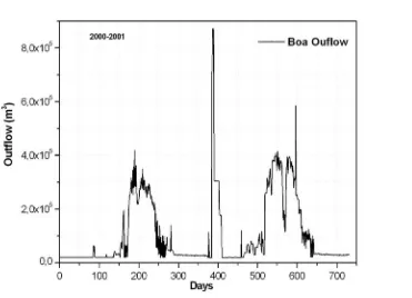
(59) Chapter 2. Figure 2.10 Daily inflow temperature (A); Daily inflow volume entering the Sau Reservoir (B).. 47.

(60) Data Analysis and Field Experiments 2.4.4 Outflow. Withdrawal of water from the Sau Reservoir including evaporation (Fig. 2.11) was higher in spring and summer due to the large volume of drinking water supply consumption occurring at those times. Additionally, high temperatures registered though the time series (2000-2001) may have increased water evaporation from the reservoir.. Figure 2.11 Daily outflow volume. 2.4.5 Sau Reservoir profiles 2.4.5.1 Temperature profiles. From Fig. 2.12 one can identify the special and temporal temperature distribution, whereas the stratification starts at the beginning of March and the formation of thermocline expending from March until the end of August. However, mixing occurs at the end December for 2000 and 2001, for the year 2001 mixing is might be due to the strong inflow river caused by the heavy rainfall recorded at the end of year 2000. Additionally, the stratification in 2000 is more or less strong than 2001 this was linked to the small storage water volume relative to the year 2001. 48.

(61) Chapter 2 During the stratified period of the year 2000 we can see that the stratification reaches the bottom. This might be due to the highest outflow of the year 2000 occurring at the beginning of June {Fig. 2.10 B}. The cooling period started after the summer stratification; this period is characterised by a deeper thermocline due to the combination of cooling surface water and wind velocity. Finally, the reservoir mixes completely in winter, producing the thermal overturning characteristic of monomictic reservoirs. The same pattern was evident in the year 2001. In the year 2000 high precipitation (Fig. 2.9) produced a high inflow (Fig. 2.10B) together with the wind (Fig. 2.8), and surface cooling enhance mixing. In the year 2001 mixing in the Sau Reservoir was similar to 2000 which is due to wind velocity which reached a maximum of approximately 9 m/s (Fig. 2.8) together with river inflow and surface cooling (Fig. 2.5, Fig. 2.8 and Fig. 2.9). Fig. 2.12 illustrates the evolution of temperature in the Sau Reservoir.. Figure 2.12 Field temperature time series. 2.4.5.2 Dissolved oxygen profiles. The evolution pattern of dissolved oxygen changed considerably from 2000 to 2001. This was due to the hypolimnion anoxic period (Fig. 2.13). The anoxic hypolimnion zone for the year 2000 started at the beginning of spring, continued through summer and lasted until approximately the end of autumn. In 2001, it started at the end of April and lasted till the end of the year. In contrast, the first river inflow at the end of February 2000 may increase dissolved oxygen content which cause the phytoplankton growth. Likewise, the highest inflow in the beginning of 2001 contributes to increase of. 49.

(62) Data Analysis and Field Experiments dissolved oxygen to 18 mg/l which was the reason of the increase in chlorophyll concentrations. For both years, the measured dissolved oxygen is presented in Fig. 2.13. In this figure the zone which is relatively high of dissolved oxygen was only a few meters from the surface layer and the anoxic zone covered the whole hypolimnion and part of the metalimnion.. Figure 2.13 Sau Reservoir time series of Observed Dissolved Oxygen. 2.4.5.3 Phosphorus. We focus here on dissolved inorganic phosphorus (Fig. 2.14). After a water treatment plant came into service in 1990 the eutrophication in the Sau Reservoir was improved considerably by diminishing the phosphorus discharge in reservoir, especially in the reservoir’s surface water. In winter, mixing occurs. The water from hypolimnion is pushed to the surface, producing a uniform phosphorus concentration, and allowing a reduction in the biologic oxygen demand in the hypolimnion as well as in 2001 the important river inflow which contains sediment load part of them was suspended solid sediment have a great impact on phytoplankton. In the stratification periods of the years 2000 and 2001, the phosphorus concentration was high on the bottom and low on the surface. In summer, therefore, the chlorophyll concentration was small, as will be seen later on. Phosphorus depletion in the surface layer indicates that this element is probably the main factor limiting the biologic activity in Sau. The other factor to be highlighted is the elevated bottom phosphorus concentration measured in the hypolimnion in the summer period and lasting until the end of the year. This therefore was due to sediment load containing in the river inflow which comes from the Sau catchment area.. 50.

(63) Chapter 2. Figure 2.14 Daily Dissolved inorganic phosphorous in the Sau Reservoir. 2.4.5.4 Chlorophyll. In January and February of the year 2000, water discharge entering the reservoir was low, resulting in a lower phosphorous concentration. However, an algal growth peak of concentration appeared in February 2000 where the inflow is negligible which induce development of phytoplankton biomass. There were two other maximum peaks in May and June. This algal growth corresponded to the beginning of the stratification period characterise by an inflow river (Fig. 2.10). The last and the most significant was in September 2000 which as well corresponding to high river inflow. Therefore, in Sau Reservoir a one can estimate in February 2000 limiting factor is light whereas in May, June and September the limiting factor is nutrient. Maximum Algal growth in 2001 was registered in October.. Figure 2.15 Sau Reservoir chlorophyll time series.. 51.

(64) Data Analysis and Field Experiments. 2.5 Boadella Reservoir data 2.5.1 Morphometry data. The. Boadella. Reservoir. (Fig.2.2). is. located. in. the. north-east. of. Spain. 42º 20´´15´Ń 2º 21´07´É . Its primary distinguishing characteristic is its small catchment area 0.182 x10 9 m 2 approximately ten times smaller than that of the Sau Reservoir. The Boadella Reservoir volume is about 0.062 x10 9 m 3 , its total surface area is 3.64 x10 6 m 2 , its maximum depth is 52 m and its altitude is 160 m above sea level (Serra et al., 2002). In Fig. 2.16 and Fig.2.17 Boadella’s area-elevation and volume-elevation data respectively are displayed.. Figure 2.16 Boadella Reservoir Area-Elevation. 52.

(65) Chapter 2. Figure 2.17 Boadella Reservoir Volume-Elevation. 2.5.2 Meteorological data 2.5.2.1 Air temperature. The air temperature over the Boadella Reservoir is a little higher than over the Sau Reservoir. The average is about 15.22ºC for 2000 and 15.42ºC for 2001. Minimum and maximum are 2.3ºC and 28.2ºC respectively for 2000 and -0.5ºC and 27.8ºC respectively for 2001. The average air temperature is plotted in Fig. 2.18.. 53.

(66) Data Analysis and Field Experiments. Figure 2.18 Boadella Reservoir air temperature time series 2.5.2.2 Solar radiation. Long-wave radiation data is not available for the Boadella Reservoir. As the hydrodynamic model requires either long-wave radiation or cloud cover, in this case we have used measured short-wave radiation (Fig. 2.19A) to estimate cloud cover (Fig. 2.19B) by interpolation between cloudy and clear sky using the following equations (Colomer, et al., 1996):. 54.