Abstract
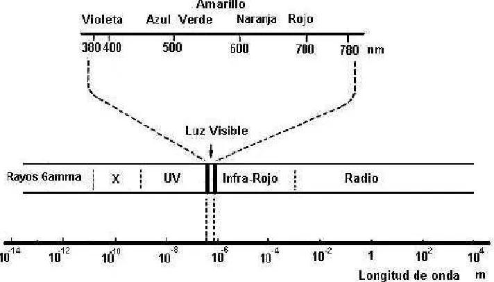
The paper describes the evaluation of visibility levels for road lighting in Tucumán, Argentina, by means of CCD image processing. The visibility is evaluated for flat standing targets of 20x20 cm with 10, 25, 35, 48 and 58% reflectance at different locations over the road.
The methodology employed, the equipment used, its calibration and the data collected for the evaluation of visibility are described. The results obtained are discussed and compared with conventional measurements and theoretical calculations.
1. Introduction
The evaluation of the visibility levels of targets over the roadway requires the measurement of target luminance, immediate surrounds luminance and background luminance. Collecting luminance data point by point from a complex image with a conventional equipment requires care and time what can be solve using a CCD camera with an image processor and a calculation software. Moreover some restrictions can appear when a luminance meter with a proper field measurement window to assure measurement over the target is not available. This was the case when the experience was build.
The target studied is a flat square object of 20 x 20 cm standing over the roadway and facing the driver's view. From the viewing position the target angular size is 7 to 11 minutes.
The CCD camera captures the scene and allows an image processing. The image is transformed in numerals, which can be correlated to photometric values. In this way a luminance
map from the image can be built and luminance over the different components can
The paper describes the methodology applied, the equipment used, the calibration and the data acquisition for visibility level evaluations. Theoretical calculations based on luminaire photometry and lighting installation geometry are compared with results from the image processing.
2. The measuring equipment 2.1 The CCD camera
A CCD (charge coupled devices) is a silicon wafer that when light photons impinge the sensitive area, accumulates charge carriers in designated discreet locations storage elements. After an integration time charge carriers are transferred under the silicon substratum toward the output records, giving rise to a new proportional charge accumulation to the incident radiation. Each storage element of the silicon is known with the name of pixel [2] [3]. For the development of a first prototype a camera, resolution 756 (H) x 581 (V) with sensitive area of 8.4 mm x 6.4mm was used [4] [5]. The pixel average angular size is 2.4 minutes.
2.2. The image acquisition board
transformation, exponential, gaussian, histogram equalization, etc. Finally, at the output, the signal goes to a digital - analogical converter (D/A) in order to be observed at a TV monitor.
The image acquisition board [6] and the image processing software [7] were installed in a personal computer. The basic operation plan of the system is shown in the figure 1.
Fig. 1: Basic system outline
2.3. Adjustment of the system " zero level " In the absence of light over the CCD detector, a signal is generated called "dark current" which has to be compensated to establish a zero reference value. This current will increase with the temperature increase of the silicon, and the visible effect of the dark current will be greater with larger exposition times.
The compensation procedure consists in acquiring one or more images with the camera lens cap onin order to avoid the luminous over the wafer of silicon. Next, an analysis of the images by means a histogram of grey level frequencies in the image area selected, obtaining the minimal, maximum and average Ng values and also their corresponding standard deviation [3]. For this experience we have measured Ngo = 6. This is the minimal useful grey level.
2.4. Spectral Analysis
The CCD spectral sensibility to the luminous
required. The above IR and under UV wavelengths radiation's should be cut off.
Former experiences showed that the system CCD – image acquisition board can have a good behaviour as a spatial resolution luminance meter [5] [8] [9], specifying a curve of L = f(Ei ,τ , α , fn , Tc [ºK],..),with a
previous spectral response correction for the CCD matching the human eye t response V(λ) of the CIE.
Fig. 2: Relative responses from CCD and from human eye according to CIE.
2.5Photometric calibration for images acquisition
A V(λ) filter [10] was incorporated to the camera, placed between the silicon wafer and the optical system in order to assure a proper response.
For the video output signal it is desirable a linear response from the photons impacts at each pixel, the function that relates the luminance L with each grey level Ng must be an expression of the form:
Ng = m L + Ngo
uniform and stable luminous opening was used. Different levels were possible with the aid of neutral filters. The absolute luminance value over the field was measured with a luminance meter.
For each image acquired a luminance L and a grey level Ng was associated for which a spot was generated. Repeating the process for different luminance levels linear regression L vs Ng was built.
The procedure was also repeated for each diaphragm apertures ƒ:
ƒ Linear regression Luminanceinterval cd/m²
error
1.4 L1.4=(Ng–5.38)/12.97 0.6<L<16 7%
2 L2 = (Ng – 5.63)/7.57 1.0<L<32 5%
2.8 L2.8= (Ng – 5.67)/4.47 1.0<L<50 3%
The conversion for the photometric analysis of any visual scene captured by the CCD camera is now possible.
3. Visibility level evaluation
Visual performance of road drivers during night relies on the amount of visual information obtained of the roadway and the surroundings. A criteria that describes an important aspect of the difficulty of the visual task is the visibility of a "critical detail" on the roadway this is usually consider to be a 20x20 cm target located at 86m in front the driver [11]. It is assume that most drivers can clear this target size; in case of bigger objects these will be more visible. The distance also assumes a safe stopping from a moderate speed and normal reaction time. Although this criterion doesn't represent all the complexity of the visual task, it is frequently used.
A target is visible when it stands out of the background, in other words when it displays a contrast that can be defined in terms of the luminance of the object. The target appears in
Luminance contrast is defined as:
where
LT : target luminance and LB : background
luminance
The visibility level VL is the number of times in which the actual target is visible related to the threshold target visibility conditions. In terms of luminance VL is obtained by the ratio of the actual luminance difference between target and background to its threshold value.
where:
Cactual: Actual target contrast = ∆Lactual / LB
Cthreshold:Threshold target
contrast=∆Lthreshold/LB ∆Lactual = LT-LB
∆Lthreshold : Threshold luminance difference between target and background
For safe and secure traffic conditions minimum maintained VL levels are recommended by CIE [12] according to the road type.
VL considers the influence of the size of the target, the contrast polarity (if it is positive or negative), the time of exposure, the age of the observers and glare. Adrian VL model [1] [13] is applied in order to calculate VL.
The equations used from the model are indicated in annex I. More details can be found in references [1], [11] and [13].
B B T L L L
C = −
Fig. 3: Negative or positive contrast for a target with α angular size
threshold actual threshold actual Ä L Ä L C C
Argentina was selected for the experience. The installation is described in figure 4.
Fig. 4: Experimental road lighting installation Luminaries photometry and lamp flux measurements were done at the lighting laboratory Depto de Luminotecnia Luz y Visión. (figure 5).
Fig. 5: Luminaire photometry from Strand MBA 70 CO, cut-off IP54. Lamp: Osram, high-pressure sodio tubular 400W.Lamp Flux: 44.861 lm.
from the road alone and with the different targets arrays were obtained from which the grey levels were transformed to spatial luminance. During the measurements voltage installation was controlled. A summary of the measured parameters and the theoretical calculated values are indicated in table 1.
Table 1: Measurements and calculations of
illuminance and luminance over a grid between two luminaries.
Source Illuminance Luminance
Pocket Lux meter
Ehave = 35 lux Ehmin = 12.9 lux Ehmax = 78.9 lux Luminance
meter
Lave = 3.4 cd/m² UO = 0.51 UL = 0.7 CCD as
luminance meter
Lave = 3.1 cd/m² UO = 0.3 UL = 0.56 Software
output
Ehave = 33.3 lux Ehmin = 12.6 lux Ehmax = 78.9 lux
Lave= 2.91 cd/m² UO = 0.35 UL = 0.72 5. Visibility levels calculated from CCD luminance measurements
The different alternatives of target positions and target surface reflectance produced 15 scenes the images of which were captured with the CCD camera. For each image grey levels were transformed in spatial luminance’s by means of the previous calibration as descripted in 2.4.
Figure 6 shows an example of the experimental installation with targets aligned at x=1.2m from the central. From the image the target’s luminance, the immediate surround luminance and the background luminance (road average luminance) were obtained in order to compute VL.
VL computed are indicated for internal line (x= 1.2m), central line (x= 6m) and external line (x= 10.8m) with the five possible target reflectance. The resulting curves are indicated Road arrangement:: Central
7. Discussion
Comparing measurements with calculations in table 4.1 it can be observed:
a)Eave, calculated, considering the existent
depreciation of 0.9 and over the same grid has a 5% difference from the measured value.
b)The Lave obtained with CCD shows an
acceptable difference within the 10% from calculated value. Similar results are found for UO and UL.
c)Target luminance's measured with CCD and calculated do not show a high correlation possibly differences in the geometry of the installation. This already well known fact is well described by Lewin [14]. Target luminance with 10% reflectance were very low to be measured with CCD therefore were not considered in the analysis.
d)Measurements of Lmed,, UO and UL with
luminance meter are indicated not as reference values provided that they were done with a 6 minutes measuring window which, produces a long oval figure on the roadway instead of a point [5]. Nevertheless the difference with CCD measured values is less than 13%. With CCD camera de average pixel size is 2.4 minutes, which allows a more precise measurement from this point of view.
In consequence the luminance measurements with CCD would be reliable in order to
At x = 1.2m VL< 7, for 35<ρ<48% in the first half of the area between two poles and for
ρ>48% in the second half. VL> 7 for targets with ρ<35% reflectance.
At x = 6m (central line) VL< 7, for 25<ρ<48% and for ρ>48% at the last tree positions. VL> 7 for targets with ρ<25% reflectance.
At x = 10.8m VL< 7 for most cases except for ρ>58% at the central positions.
Even if the installation fulfils the CIE recommendations for luminance levels recommendations [5], zones would exist where the visibility could be VL< 7 according to the target reflection considered.
8. Conclusions
The utilisation of CCD as a luminance meter in order to calculate VL has big advantages because it reduces the time required for the luminance distribution measurements and allows a more fine analysis from the image details. With conventional luminance meter some details could escape of the analysis or positional errors could appear. There are still limitations concerning with the reliably with low levels especially under 0.7 cd/m². This range has probably been reduced from the time the experience was done as CCD technology has improved.
9. Acknowledgements
The authors wish to thank to the Universidad Nacional de Tucuman and CONICET from Argentina for the research financial support. To Arce J. from the ILLyV for the luminaries photometry. To the Municipal authorities and to Alvarez M. from SIE lighting maintenance Co. for the aid during the experience and finally to the Universitat Politècnica de Catalunya and Universidad de Valladolid both from Spain where the paper was written. Fig. 6: Road lighting installation array with
-60 -50 -40 -30 -20 -10 0 10 20
0 4 8 12 16 20 24 28 32 36
y [m]
VL
VL(58%)
-45 -35 -25 -15 -5 5 15 25 35 45
0 4 8 12 16 20 24 28 32 36
y [m]
VL
VL(25%)
VL(35%)
VL(48%)
VL(58%)
-35 -25 -15 -5 5 15 25 35 45
VL
VL(25%)
VL(35%)
VL(48%)
VL(58%)
surface reflection 25, 35, 48 and 58 %.
Figure 8: VL calculated from luminance measured with CCD at x = 6m with target surface reflection 25, 35, 48 and 58 %.
2 2 / 1 2 / 1 .6 2 + Φ ⋅ L α
(
L) (
a L)
AFF
L ⋅ CP B ⋅ B ⋅ + Φ ⋅ =
∆L 2.6 , . ,
2 2 / 1 2 / 1
threshold α α
α
where:
is the threshold luminance difference for positive contrast, observer average age 23 years and a 2 sec or unlimited observation time. This is a function of size (Ricco and Weber) and background luminance.
For LB≥ 0.6 cd/m²
5867 0 1556
0 2
1 log 41925 01684 .
B . B / L . ) L . ( Ö = ⋅ + 466 . 0 2 /
1 0.05946
B L
L = ⋅
For 0.00418 cd/m² < LB < 0.6 cd/m²
(
)
21/2 0.072 0.3372 log 0.0866log
Ö
log = + ⋅ LB + LB
B L
L 1.256 0.319 log
log 1/2 =− + ⋅
α : Target angular size [minutes]. A circular target with radius r seen from distance d has
an angular size:
: contrast polarity factor. Is 1 for positive contrast and less than 1 for negative as targets are more visible. Where m
comes from:
( )
(
log 12 0.0245)
10
logm=− −K⋅ LB+ +
K=0.125 for LB > 0.1 cd/m²
K=0.075 for LB > 0.004 cd/m² 1488
. 0 6 .
0 ⋅ −
= LB
β for any LB
: exposure time . influence
( )
= − − ⋅ ⋅ + 28 . 52 4 . 10 1217 . 0 355 . 0 2 B B B L a F(
log +6)
= LF
B
AF : influence of age
23y < age < 64y
(
)
0.992160 192 + − = age AF
64y< age < 75y
(
)
1.433 . 116 6 . 56 2 + − = age AF
11. Authors reference
#
Universidad Nacional de Tucumán,
Departamento de Luminotecnia Luz y Visión “H.C. Bühler”, Av. Independencia 1800 (4000) Tucumán, Argentina.
†
On leave at Universitat Politècnica de
Catalunya, Dept. Projectes d’Enginyeria, ETSEIB, Av. Diagonal 647, 08028 Barcelona, Spain. Fax:+34 3 3340255.Email: [email protected]
‡
On leave at Universidad de Valladolid,
Departamento de Optica, Facultad de Ciencias 47071-Prado de la Magdalena s/n, Valladolid, Spain. Fax: +34 83 423013.
Email: [email protected]
12. References [1] Adrian W.
The physiological basis of the visibility concept Proceeding of the 2nd International Symposium on Visibility an Luminance in Road Lighting. page 17-30 Orlando USA.
October 1993 [2] Karim M.A
Electro-optical Devices and Systems
chapter.4, page 152, PWS-Kent Publishing Company,
1990
[3] Jenkins T.E.
Optical Sensing Techniques and Signal Processing chapter.4, page 74, Prentice-Hall,
1987 [4] Pulnix
Camera, model TM - 765.
( )
602⋅ 1 ⋅
= − d r tan α
(
)
POS F CP L m L F ∆ ⋅ ⋅ − = − 4 . 2 1 , α β α(
)
[
( )
( )
]
1 . 2 , 2 / 1 2 2 F F L a a LImage acquisition board by Imaging Technology Inc.
[7] Ipplus
Image processing software
[8] Grupo de Investigación en Fotometría
Luminancímetro con Resolución Espacial: Calibrado y Aplicaciones. Informe del Dpto. de Optica, Cátedra Física Aplicada III, Universidad de Valladolid, España.
Noviembre 1991. [9] Rea M.S., Jeffrey I.G
A New Luminance and Image Analysis System for Lighting and Vision I. Equipment and Calibration, Journal of the Illuminating Engineering Society, pages 64-72,
1990
[10] PRC Krochmann
V (λ) filter. http://www.ingenieur.de/prc/ [11] Adrian W.
Visibility Levels under night-time driving conditions
Journal of the Illuminating Engineering Society Summer 1987
[12] Commission Internacionale de L'Eclairage. Technical, report: Recommendations for the lighting of roads for motor and pedestrian traffic. Public. 115. http://www.cie.co.at/cie/
1995
[13] Adrian W.
Visibility of targets: Model of calculation
Lighting research and Technology 21, page. 181-188
1989
[14] Lewin Ian
Measurements of STV-VL and the reasons for possible deviations
*Universitat Politecnica de Catalunya, Depto. Projectes de L’Enginyeria, ETSEIB, Av. Diagonal 647, 08028 Barcelona, Espanya. Email: [email protected]
‡ Universidad Nacional de Tucumán, Instituto. de Luminotecnia Luz y Visión, Av. Independencia
1800, 4000 Tucumán, Argentina, Email: [email protected], Fax:+ 34 93 334 02 55
1. Resumen
Bajo el punto de vista energético, una instalación de alumbrado es una importante fuente de consumo de energía, que se produce en la fase de explotación y se ve afectado por factores tales como maniobra, regulación, mantenimiento, etc. Si bien las características técnicas de la instalación de alumbrado es un primer determinante de la eficiencia energética, la verdadera racionalización del consumo solo puede conseguirse con una gestión eficaz de la explotación. La explotación de instalaciones de alumbrado presenta características singulares (variación de periodos de uso, depreciación de luminarias, agresión ambiental...) las cuales junto a la descentralización geográfica del alumbrado público dificultan la correcta gestión. Por lo tanto, existe un elevado potencial de ahorro energético en el diseño de las políticas de gestión de la explotación de instalaciones.
La comunicación describe las acciones que en este sentido realiza el equipo de Estudios Luminotecnicos de la UPC (Auditora, Plan Director, Informática de Gestión, etc.) como así también las investigaciones en curso para optimizar el diseño de las políticas de gestión.
2. Introducción
El mayor efecto de las instalaciones de alumbrado en el impacto ambiental se produce en la explotación, durante su vida útil. Las consecuencias mas importantes pueden agruparse en:
a) Producción de dióxido de carbono (efecto invernadero) y otros elementos por generación de energía eléctrica que afectan el medio ambiente y que pueden minimizarse con un consumo eficiente.
b) Eliminación periódica de ciertos componentes de las instalaciones como las lámparas, que contienen mercurio no deseable, sin embargo su presencia, por ahora, hace eficiente su funcionamiento desde el punto de vista energético. Reducir la cantidad de componentes con sustancias contaminantes es también un objetivo del diseño eficiente. c) Contaminación lumínica, visible como brillo nocturno de la bóveda celeste producido
por la dispersión de la luz en la atmósfera lo que impide la visión directa o astronómica de las estrellas. Existen medidas practicas para minimizar su efecto, se basan en evitar la emisión de luz por arriba de la horizontal, orientando todo proyector hacia abajo preferentemente y principalmente en el empleo de luminarias con reducida emisión del flujo hacia arriba.
d) Efectos en el crecimiento, hábitat de especies animales y vegetales. La regulación en el uso o el apagado total en determinados períodos reduce este efecto.
esfuerzos por considerar aspectos relacionados con la gestión y explotación debido a que afectan posteriormente la calidad del servicio, el consumo energético y en consecuencia el medio ambiente. Un enfoque mas global considera además el ciclo de vida completo, donde operación, gestión, mantenimiento, consumo energético, eliminación, etc. están involucrados y relacionados. Bajo esta óptica en el diseño del alumbrado se deben considerar una serie de aspectos [1] de los cuales por razones de espacio destacamos los siguientes:
• Condiciones de iluminación y régimen de funcionamiento adecuadas.
• Selección de los sistemas técnicos eficientes
• Dimensionamiento y calculo considerando la depreciación de las instalaciones y la política de mantenimiento a implementar.
3.1 Condiciones de iluminación apropiadas
Crear condiciones apropiadas de iluminación significa satisfacer aspectos funcionales y de confort de los usuarios a un costo razonable, que se mantengan durante el transcurso de la vida útil de las instalaciones, lo cual puede preverse en la etapa del diseño. Los aspectos funcionales pueden quedar garantizados con un nivel elevado de iluminación sin embargo esto determinaría un elevado consumo energético. Es necesario establecer una escala de niveles acorde a la exigencia visual y a las características de la zona a iluminar. Los criterios para establecer el escalonamiento se basan en:
• tipo de usuarios: peatones, conductores, mixtos.
• características del tráfico: densidad y velocidad de vehículos, densidad de peatones
• características ambientales: percepción del espacio, seguridad ciudadana
Simultáneamente es importante lograr cierta uniformidad por seguridad y reducir posibles brillos intensos que pueda producir la instalación para evitar afectar la visibilidad y el confort visual. Al respecto existen recomendaciones para el diseño [2] [3].
La posibilidad de regulación del régimen de funcionamiento, reduciendo niveles de iluminación en determinadas horas nocturnas es una alternativa para racionalizar energía. Contemplada en la etapa del diseño puede implicar menores costos comparado con modificaciones o agregados sobre obras existentes. Pero antes de decidir la implantación es preciso estudiar dos aspectos:
a) que la reducción del nivel de una zona sea como consecuencia de una reducción de las exigencias visuales (por ejemplo reducción de la densidad de trafico o presencia de peatones) y que no este acompañada de un efecto indirecto como aumento de la inseguridad ciudadana.
b) que la aplicación del sistema sea rentable, dado que el costo suplementario debe amortizarse (3 a 5 años) con la reducción del costo energético obtenido aun cuando el uso sea en horas valle donde el costo de la energía es mas bajo.
3.2 Sistemas de iluminación e instalaciones eficientes
cuando mayor sea, menor será el consumo energético para lograr la misma iluminación. La eficiencia usualmente no esta asociada a la buena reproducción del color, en situaciones donde prime el color, el criterio de decisión se puede alterar. Aún así gradualmente las lámparas de mayor eficacia, como las de Sodio de alta presión reemplazan a las de Mercurio color corregido de menor eficacia pero con mejor respuesta al color. Un
remplazo completo posiblemente tenga un límite dado a la existencia de zonas comerciales, residenciales etc. donde la preferencia es el color. La distribución actual en Cataluña se indica en tabla 1.
La eficiencia de la luminaria depende de cuan efectivo sea su óptica (reflector, refractor etc.) en orientar el flujo luminoso de la lámpara sobre la zona útil u objetos de interés. El flujo es mas sencillo de controlar en lámparas tubulares por el reducido tamaño que en lámparas extensas u ovoides con recubrimientos de polvo fluorescente interior. La altura de montaje y orientación afectan también la eficiencia del conjunto. El porcentaje de flujo luminoso útil proyectado sobre la calzada respecto del emitido por la lámpara cuantifica la eficiencia lumínica lo que asegura de algún modo la mejor visibilidad. Parte del flujo luminoso también es necesario para crear un entorno visual atractivo limitando brillos perturbadores o molestos, no obstante conviene limitar la innecesaria emisión hacia el cielo. La geometría de la instalación puede afectar la explotación y la facilidad de mantenimiento. La situación de los puntos de luz , altura , han de fijarse favoreciendo el acceso, control y mantenimiento de otro modo la depreciación crecerá con el tiempo y con ella la reducción de las condiciones de iluminación derrochando energía (ver 3.3).
Una instalación de alumbrado público eficiente es el resultado de la combinación de lámpara, luminaria, geometría y política de mantenimiento adecuado. En este sentido se
efectuó un estudio comparativo de distintas alternativas evaluando costos de instalación,
mantenimiento, consumo energético y emisión de flujo hacia al cielo. Los resultados se indican en la tabla 2 [4]. En todos los casos las condiciones de iluminación fueron similares (ver figura 1). La emisión de flujo hacia el cielo (∅c)calculada es el resultado de la emisión directa al cielo mas la reflejada en la calzada y fachadas cercanas considerando la instalación dentro de un recinto formado por la calle y edificios laterales (ver fig. 1).
Figura 1: Condiciones de iluminación que debían producir las instalaciones analizadas
De tabla 2, se observa que los sistemas mas ineficientes emplean luminarias de alumbrado indirecto (caso 12) con parte del haz luminoso proyectado hacia arriba. Comportamiento similar muestran las luminarias tipo globo, que emiten también una gran proporción de flujo Tabla 1: Porcentaje de lámparas instaladas en 31 Ayuntamientos encuestados en Cataluña, 1998.
Mercurio CC 50 65
Merc. c/halog. 90-100 3
Otras < 40 5
Lmed: luminancia media = 1cd/m²
UO = Lmín/Lmed ≥ 0,4 (uniformidad general)
UL = Lmín/Lmáx≥ 0,7 (longitudinal)
G ≥ 5
TI% ≤ 20%
Pavimento: R3
el flujo hacia la calzada, requiriendo menores separaciones entre luminarias, por el contrario una distribución de flujo algo mas amplia en sentido longitudinal a la calzada indica ser mas económica durante la vida útil de la instalación y con menor emisión de flujo hacia el cielo (caso 7).
Costos relativos por Km y año
Nº Luminaria Cierre Lámpara Instala-ción##
Manteni-miento† Energía‡ Total
Flujo al cielo
KLm/Km
1 Sap 150wTubular 107 103 103 104 28.6
2
vidrio
curvo Sap 150w
Ovoidal 140 135 135 137 32.2
3 Sap 150wTubular 112 117 117 115 31.6
4
vidrio
plano Sap 150w
Ovoidal 177 184 184 182 31.6
5 Sap 150wTubular 111 117 117 115 31.2
6
cubeta
poli-carbonato Sap 150w
Ovoidal 208 219 219 215 35.8
7 Sap 150wTubular 100 100 100 100 26.8
8
vidrio
prismático Sap 150w
Ovoidal 159 159 159 159 33.2
9 polímerocubeta acrílico
Sox 90w 138 125 75 108 37.0
10
polímero cónico
tapa reflectora
Sap 150w
Ovoidal 151 175 175 166 61.8
11 globo poli-carbonato Sap 150wOvoidal 194 250 250 229 200.0
12
Proyector con pantalla reflectora
Sap 250w
Tubular 525 438 729 595 326.0
## : Incluye suministro, materiales, mano de obra, beneficio,IVA,imprevistos, gastos adm.etc. y amortización en 25 años
† : Costo anual fijo por punto de luz
‡ : Costo de la energía promedio 15 Ptas/Kw
ensuciamiento de los componentes, la instalación se deprecia gradualmente. Para mantener los niveles por arriba del mínimo recomendado se debe combinar la selección de los componentes, con el dimensionamiento de la instalación (cantidad de puntos de luz) y con estrategias de reposición y limpieza adecuadas durante la vida útil de las instalaciones. En la fig. 2 se ejemplifica la variación temporal teórica del nivel de iluminación con reposiciones masivas programadas cada tres años [5] y una limpieza anual. Un factor de depreciación se elige en función de los períodos de limpieza y mantenimiento que se realizará sobre la instalación a lo largo de su vida útil para compensar inicialmente la reducción gradual por depreciación. En la fig 2, para mantener las condiciones de iluminación, se debe diseñar la instalación incrementando un 25% aproximadamente los puntos de luz.
El empleo de luminarias que sufren una depreciación mas acelerada (caso 12), debido a la acumulación de polvo en superficies emisoras de luz horizontales obligan al empleo de una mayor cantidad de puntos de luz (mayor nivel de iluminación inicial) para compensar la depreciación gradual hasta el mantenimiento correspondiente o en su defecto un mantenimiento mas frecuente es necesario.
La realización de cálculos luminotecnicos en forma fiable permite dimensionar el sistema de alumbrado con unos márgenes de seguridad mas ajustados con soluciones económicamente mas favorables para la explotación. El empleo de software de calculo y la aplicación de técnicas mas sofisticadas y realistas, (como la técnica de la Luminancia que tiene en cuenta la reflexión del pavimento) son cada vez mas frecuentes en los proyectos de alumbrado.
0.60 0.65 0.70 0.75 0.80 0.85 0.90 0.95 1.00
0 4 8 12 16 20 24 28 32 36 40 44 48 52 56 60
Tiempo trancurrido [meses]
% del valor inicial
Depreciación del flujo de la lámpara Supervivencia de la Lámpara Depreciación del artefacto Artefacto después de la limpieza Evolución del flujo de la Luminaria
Lámpara :Sodio AP 250W Luminaria :IP 54
Periodo de sustitucion masiva de lámparas: 36 [meses] Porcentaje de sustitucion: 100
[image:13.595.113.511.264.526.2]Periodo de limpieza masiva: 12 [meses]
energéticos y por tanto en ahorros económicos importantes. Dejando de lado las medidas estrictamente tecnológicas, una herramienta importante en la mejora de la eficiencia energética es la gestión de las instalaciones. Como resultado de diversos estudios realizados se observa que no existe en la mayoría de los casos una gestión del alumbrado. Este hecho se constata en la ineficiencia energética generalizada en los sistemas en funcionamiento.
La gestión integrada del alumbrado debe contemplar tanto la gestión energética como el mantenimiento de las instalaciones. El primer problema que origina la falta de gestión es el desconocimiento de las instalaciones, la inexistencia de inventarios operativos y actualizados impide cualquier intento de control o planificación de tareas de mantenimiento. La ausencia de gestión origina los problemas de ineficiencia energética, los principales aspectos en que ésta se manifiesta son:
• Incorrecto funcionamiento de los dispositivos de maniobra y control.
• Perdidas por depreciación lumínica.
• Aparición de consumo de energía reactiva no deseable.
• Sobreconsumo debido a sobretensión de las líneas eléctricas.
Además de los problemas estrictamente energéticos, también se originan:
• Perdidas en la calidad del servicio.
• Aumento de la tasa de averías, con el consecuente aumento del coste del mantenimiento.
• Incorrecta contratación de tarifas eléctricas, lo cual penaliza económicamente.
Como ejemplo de la problemática citada aportamos algunos datos correspondientes a una población mediana de Catalunya con 2300 puntos de luz.
4.2.- Políticas y gestión administrativa, empresas municipales y contratadas.
Dos opciones para la gestión y explotación de las instalaciones de alumbrado son aplicadas en general: los servicios técnicos municipales con su brigada propia y/o la empresa subcontratada de mantenimiento. Debido a la tendencia actual de reducción de personal municipal, sumado al aumento en la complejidad técnica de los sistemas de alumbrado se ha visto incrementado el número de poblaciones con empresas de mantenimiento subcontratadas. Pero ocurre que el servicio de mantenimiento no incluye la gestión energética aún cuando es ofrecido por las empresas contratadas debido a falta de interés por parte de los ayuntamientos posiblemente por temor a perder el control sobre sus instalaciones.
Problema consumo anualAumento del Aumento delcoste anual Sobreconsumoenergético
Desajuste de
horarios 304 Mwh/año 4.9 Mpts/año +27% Consumo de
energía reactiva 103 MVAr/año 1.3 Mpts/año Ineficiencia de
el técnico municipal imposibilita dedicar el tiempo suficiente a las tareas de gestión energética y planificación del mantenimiento.
Dadas las ventajas e inconvenientes de cada modalidad de mantenimiento y debido a las distintas características de cada municipio, cada caso requiere de un minucioso estudio. Aunque la situación parece claramente a favor de la subcontratación del la gestión y explotación de las instalaciones de alumbrado, las tareas de gestión energética y control de calidad, se aconseja sean realizadas por el propio ayuntamiento o por un tercera entidad independiente.
4.3.- Ventajas de las auditorías energéticas y planes directores de alumbrado.
Una Auditoria Energética de Alumbrado Público, establece un diagnóstico objetivo de la situación actual del alumbrado. Partiendo de los datos de la información básica obtenida del propio ayuntamiento como de las propias instalaciones, se detectan las posibles correcciones de las instalaciones desde el punto de vista energético. Generalmente la Auditoria Energética viene acompañada de un plan de adecuación que contempla las propuestas de mejora con su correspondiente valoración económica. De hecho, la auditoria energética se convierte en un valioso documento tanto para validar las instalaciones y su gestión, como para detectar posibles problemas y plantear propuestas de mejora. También es una herramienta aconsejable como punto de partida para iniciar una gestión y explotación correcta de las instalaciones en aquellas entidades donde todavía no se realiza.
Un Plan Director de alumbrado, es un conjunto de acciones que partiendo de la situación del alumbrado existente en una población , establece las actuaciones a seguir a largo plazo con el fin de adecuar el alumbrado a las exigencias técnicas y características urbanísticas de la población. El Plan Director establece unos plazos de ejecución de mejoras ajustándose a las posibilidades de inversión anual del municipio. La principal ventaja que obtiene el municipio es el conocimiento exacto de cuales son las carencias y el camino correcto para solventarlas. Al contemplar el alumbrado de la población como un todo y no como un conjunto de instalaciones aisladas , se obtiene una visión global de como debe ser el alumbrado de la población. Los criterios de partida para la confección del plan son diversos. Intentando cubrir las necesidades lumínicas de la población contemplando la eficiencia energética, requisitos estéticos, urbanísticos, de utilización etc.
5. Herramientas de la gestión del Alumbrado Público. 5.1. La Gestión Continuada.
parámetros energéticos a modo de consulta en el propio ayuntamiento.
• Futura posibilidad de intercambiar información con el “Gestor Energético” vía internet.
5.2. Informática de gestión del alumbrado público.
Las aplicaciones informáticas se han convertido en una herramienta insustituible para la gestión del alumbrado. La mejora viene dada por la facilidad que permiten para tratar gran cantidad de información. En los programas desarrollados por el Equipo de Estudios
Luminotécnicos de la UPC se han tenido en cuenta todos los aspectos para la gestión
integral del alumbrado público, estos aspectos son:
• Inventario alfanumérico de las instalaciones con sus características concretas.
• Modulo de gestión energética, para almacenar datos históricos y su análisis gráfico.
• Control sobre el mantenimiento correctivo de las instalaciones.
• Programación del mantenimiento preventivo.
• Gestión de stocks.
La aplicación alfanumérica esta asociada aun módulo cartográfico, que una vez digitalizado el plano de la población e introducidas las instalaciones interacciona con la aplicación alfanumérica. Esto tiene la ventaja de ofrecer mayor versatilidad y un manejo más intuitivo de los programas. Estas aplicaciones ya se encuentran instaladas en tres poblaciones, funcionando satisfactoriamente según las expectativas previstas.
Juntamente con las dos aplicaciones en funcionamiento, gracias a la proliferación de la telegestión en los elementos de maniobra en las nuevas instalaciones, se están desarrollando nuevas aplicaciones que aprovechen esta circunstancia. Estos nuevos desarrollos permitirán la interacción entre los datos recibidos de los cuadros de maniobra con los programas de gestión actuales. La gran ventaja de estos nuevos desarrollos será el de poseer y analizar la información de los parámetros eléctricos en tiempo real. Esta circunstancia permitirá actuar con mayor rapidez para corregir las ineficiencias detectadas.
5.3 Metodología de evaluación de la calidad del servicio
Con el fin de optimizar la gestión y explotación de instalaciones de alumbrado o detectar desviaciones se trabaja actualmente en un proyecto para desarrollar una metodología que cuantifique el nivel de servicio del alumbrado público. Consiste en relacionar costos y beneficios (o eficacia) que producen durante la vida útil las instalaciones, desde la etapa de proyecto e instalación, durante la explotación y el mantenimiento hasta la eliminación. Es conocida, desde el punto de vista energético, que mínimos costos no significan mayores beneficios. El empleo de la relación costos – beneficios tiene tres objetivos que establecen además distintos niveles de aplicación y dificultad:
a) Comparar instalaciones alternativas en la etapa de proyecto de las instalaciones
b) Evaluar rápidamente, con limitados parámetros la calidad del servicio en una población comparando políticas alternativas de mantenimiento actuando como complemento de soportes informáticos de gestión
acuerdo al comportamiento teórico de los componentes. Paralelamente se estudia la tasa de fallos de componentes principales. Como fuente de datos se dispone de encuestas a ayuntamientos, inspecciones y datos históricos de empresas de mantenimiento.
Como ejemplo, de un factor vinculado a la gestión energética, el coste de la energía representado en la fig. 5.1 en función del tipo de tarifa contratada y del porcentaje de regulación de la potencia de las lámparas [6]. Hasta el 40% de regulación, 2.0 T0 es la tarifa más económica no obstante sobre 31 ayuntamientos encuestados sólo un 19% la contrata [7].
Por su parte el beneficio del alumbrado consiste en proveer condiciones apropiadas de visión para la seguridad vial y ciudadana creando un ambiente animado y confortable de uso. La cuantificación y correlación de estos aspectos con la calidad del servicio del alumbrado es complicada, motivo por el cual se ha buscado un indicador operativo relacionando un parámetro funcional del
nivel del alumbrado, sobre el área de interés, durante el tiempo de operación necesario del servicio, considerando la confiabilidad, frecuencia y duración de fallas, la seguridad eléctrica y mecánica del sistema, y la apariencia de la instalación (estética, color de la luz). Un análisis global permitirá efectuar un seguimiento de la evolución cubriendo el ciclo de vida de la instalación que puede variar entre 15 y 20 años. Los costos financieros del capital invertido junto a los gastos operativos, de explotación y eliminación serán trasladados a un valor presente constante para poder comparar en cualquier instante su evolución.
6. Aportes al medio
Durante los últimos años, diversos estudios y realizaciones prácticas se han realizado con el fin de mejorar la eficiencia energética en el alumbrado público, que se resumen a continuación según el tipo de actuación:
Auditorias energéticas: Alrededor de 20 auditorias energéticas posibilitan tener un
conocimiento de primera mano de la problemática energética en las instalaciones de alumbrado público. La incidencia de estos estudios ha posibilitado mejorar la eficiencia de sus instalaciones. En un reciente seguimiento de los estudios realizados, se ha constatado el grado de aplicación de las medidas correctoras. Las cifras exactas de ahorro energético conseguido en la implantación de las propuestas de mejora es del 60% , es decir, las propuestas de mejora aplicadas por los municipios han supuesto este ahorro energético sobre el total estimado en los estudios realizados.
13.00 13.50 14.00 14.50 15.00 15.50 16.00 16.50 17.00
0% 10% 20% 30% 40% 50%
Porcentaje de regulación de potencia
energía [ Ptas.] (1997) 3.0 T3 4.0 T3 4.0 T4 2.0 T0 B.0
Potencia contratada 15 Kw Costo del contador 3000 Ptas.
Potencia reactiva 0%
Regulación 24:00 hs hasta apagado
3%
2%
19%
75%
Gestión Continuada: En la actualidad el Equipo de Estudios Luminotécnicos aplica este sistema en una población a modo de experiencia piloto. El poco tiempo desde el inicio de esta experiencia no posibilita tener datos fiables, aunque todo apunta hacia unos excelentes resultados futuros.
Plan de Acción de las instalaciones de Alumbrado Público de Girona: En 1997 se inició
un plan de acción de las instalaciones de alumbrado de Girona. La primera fase ya finalizada, ha consistido en la realización de un completo inventario informatizado de las instalaciones, acompañado del desarrollo de un programa de gestión del alumbrado público. Los resultados hasta el momento son satisfactorios, habiéndose iniciado una dinámica de gestión que en un futuro se traducirá en un tangible ahorro energético. Como segunda fase del plan de acción se iniciara en breve la confección del Plan Director de las instalaciones de Alumbrado Público.
7. Conclusiones
El consumo energético del alumbrado representa una porción notable del total de energía eléctrica (alrededor del 20%) que sufre además un crecimiento exponencial, tanto en la extensión de las instalaciones como en los niveles de potencia utilizados.
Mucho se ha avanzado y se continua, en el desarrollo de fuentes de luz de elevada eficacia, luminarias de alto rendimiento, técnicas de calculo y diseño precisas, lo que permite reducir la potencia instalada necesaria. Pero energía es potencia en el tiempo y en este segundo factor la gestión de uso es donde se puede conseguir ahorros energéticos que por otra parte van a reducir el impacto ambiental de las instalaciones de alumbrado.
8. Referencias
[1] San Martín, R. / Manzano E.
“Gestión y explotación de instalaciones: aspectos a considerar en la elaboración de proyectos”, Actas del XIII Congreso Nacional de Ingeniería de Proyectos, Volumen II, pág. 919 a 925. ISBN : 84-88783-30-2. Sevilla, España.
Noviembre 1997 [2] San Martín R.
Auditoría energetica I, Enllumenat públic.
Diputacio de Barcelona, Servei del Medi Ambient, ISBN 84 505 2352 4 1985 [3] International Commission on Illumination
Recomendation for the lighting of roads for motor and pedestrian traffic, Pub.Nº 115 1995 [4] Borras J.
Projecte final de carrera en curs, Departament Projectes d’Enginyería, Universitat Politècnica de Catalunya. Dirigit per Dr. San Martín R. i Manzano E.. 1998
[5] Manzano E.
Metodología para evaluar la calidad del servicio
Trabajo de tesis en curso. Departament Projectes d’Enginyería, Universitat Politecnica de Catalunya. 1998
[6] Saro O.
Software de simulación de tarifas, Grupo de Estudis Luminotecnicos, Universitat Politecnica de Catalunya 1997
ABSTRACT
In order to evaluate the urban lighting management., a procedure based on the benefit/cost of operation relationship is described. Taking into account several types of facilities under different management and maintenance policies field surveys were carried on in order to correlate cost and benefits. The collected data as well as historical data from lighting maintenance companies were analysed to formulate and test the proposed procedure. A quantification of the benefit based in factors as the lighting level, the permanent failure rate, the lighting system operation time, etc, is proposed. The management planning, based on a simple procedure, allows the application of a maintenance policy which can be subsequently adjusted with control data. Finally, results of the application on a existing installation are described.
1. INTRODUCTION
The aim of urban lighting is to provide a service to the citizens. This service is restricted on one hand by installation performance features, (designee and equipment) and on the other hand by the use that is made of it. Whereas the performance features are determined at the project stage the usage is established during management, that is control, maintenance, etc.
In practice it can be seen that service conditions are variable, according to the different management policies adopted, situation that often leads to a reduction of service conditions, higher costs, or to a lower profitability of the invested resources, when all these conditions are not given simultaneously. The origin of these situations can be due to:
•lack of concern about the real conditions of the
service installations
•limitations of the necessary economical resources
invested, whether for the project or the operational phases
•difficulties on the definition of appropriate
criteria and policies
The last two are deeply related to the lack of service quantification level, since they make the decision depend exclusively on cost factors and
avoid the positive motivations based on the improvement of the service.
The objective of the paper is to establish the bases of a decision and control procedures permitting to guarantee an adequate service level and at the same time to make the economical resources invested efficiently profitable. The procedure would be
based in the application of benefit/cost criteria for
the optimisation of the decisions and as a way of
controlling the results.
2. DATA ANALISYS
In order to evaluate the state of lighting management and its relation with service conditions a series of studies and experiences have
been made: a) compilation and analysis of data
tending to evaluate the effect of the lack of
management over energetic costs, b) surveys to
the lighting managers to determine characteristics of the installations (lamps type, luminaries, age, number), maintenance policy, budget, types of
contracted tariffs, etc., c) evaluation of the state of
installations operation, d) analysis of data bases
from historical records of lighting installations maintenance operations.
The results of greatest interest for this study are now summarised.
a) Energy costs experience variations with respect
to normal values due to lack of management and maintenance. Increases in active energy consumption due to over-voltage and lack of maintenance in control switch devices, reactive energy consumption and inappropriate tariff contracts, cause increases of urban lighting costs. These factors and their effects are analysed in a previous paper [1].
b) The maintenance policies frequently applied are:
iluminance over the road (Ehave) before and after cleaning luminaries and lamp replacement was measured at representative streets. The installations
had luminaries with IP54 or greater. At villages Be
(3.500 inhabitants/900 luminaries) and StB (80.000 inhabitants/6.300 luminaries), both with corrective
(includes spot lamp replacement, SR) and preventive policies (every 2 years group lamp replacement, GR and group luminaire cleaning GC) done by external maintenance contractor, the
observed average depreciation (relation of Ehave
before and after cleaning and lamp replacement)
was 0,9; while for village EM (1.800
luminarie/20.000 inhabitants), with only corrective
policy (SR) done with their own resources, the
[image:20.595.313.508.71.218.2]average depreciation was 0,6 (Fig. 1).
Figure 1: Influence of lighting management strategies over the maintenance factor. SR: spot lamp replacement, GR+GC: Group lamp replacement and luminaire cleaning.
d) The number of failed lamps regarding to the
installed ones in a random sample of streets has been used as an estimator of the percentage of permanent failed luminaries (PFL). In Fig. 2 the frequency distribution of PFL is indicated for 21 village's survey from Catalunya, Spain. The observed average is 2.9 %. However, in villages us
Be and StB, with appropriate maintenance PFL is
lower than 1%.
The accumulated effect of depreciation and PFL produces up to 30 % of difference in the quality service according to the applied policy.
e) Data covering a period of 6 years (92-98), from
a city where a maintenance Co. employing a policy with SR, GR every 3 years, and GC every 2 years, were analysed.
[image:20.595.95.284.327.481.2]A review of the different maintenance operations performed are shown in Table 1. 72% of the corrective maintenance operations occur at light points (luminaire+control gear+column+fuse etc.) were of these, 54% corresponded to lamp failures, which is indicative of the importance of this component in the evaluation of costs and security of service.
Table 1: Distribution of maintenance operations for urban lighting installations from data analysis.
Operations Preventive 50%
Light points 72%
Control panels 25%
Corrective
maintenance 50% Electric wiring
3% Total 100% 100%
Analysing the time passed from a GR until the first spot lamp replacement occurs (failure between GR, excluding vandalism and false contacts), survival curves are obtained under actual burning conditions. Results obtained are indicated in Fig. 3 for C.C. mercury lamps (Merc.) and in Fig. 4 for high pressure sodium lamps (HPS).
Figure 3: Lamp survival data for 80 125, 250, 400W mercury lamps with Weibull regression functions. And average manufacturer LSF.
Figure 2: Frequency distribution of percentage of permanent failed lamps (PFL) at 21 villages in Catalunya, Spain [2].
0 1 2
1 2 3 4 5 6 7 8 9 10
% permanent failed lamps .% 20.% 40.% 0 5 10 15 20 25 30 35 40 45 50
0.0-0.1 0.1-0.2 0.2-0.3 0.3-0.4 0.4-0.5 0.5-0.6 0.6-0.7 0.7-0.8 0.8-0.9 0.9-1.0
% of observed values
SR+GR+GC every 2 years
SR 0.3 0.4 0.5 0.6 0.7 0.8 0.9 1.0
0 2000 4000 6000 8000 10000 12000 14000 16000 18000
[image:20.595.315.508.386.455.2]Figure 4: Lamp survival data for HPS 150, 250, 400W lamps with Weibull regression functions and average manufacturers LSF.
Regarding the behaviour indicated during manufacturer tests, noticeable differences can be observed possibly due to the fact that actual burning conditions differ from those under laboratory tests.
From the results it can be deduced that in practice a great variability of conditions appear, leading to a deviation from theoretical behaviour.
A service level quantifying indicator would permit and evaluation, which if necessary, could be complemented with a study of each factor in particular.
3. BENEFIT/COST RATIO
A procedure based on the determination of the ratio benefits /annual operation costs, for planning and controlling lighting management, requires to establish which are the benefits and costs and to quantify both.
The benefit for citizen and road drivers from urban lighting is to find appropriate visual conditions to proceed safety, creating an ambient of security and comfortable use. Quantifying these aspects presents certain difficulty, this is why it is convenient to look for a more operative indicator relating, lighting level (K(E)), the necessary
operation time (K(TO)), reliability and failure
duration (K(PFL)), and other aspects like the electrical and mechanical safety of the system (K(S)), the appearance of the installation (aesthetics, light colour, etc) (K(A)), and the illuminated area (A). The benefit can be defined as the multiplication of these factors, where the relative weight of each one is considered the same for the moment.
K(E) depends of the road average iluminance (E), which limitations, in spite to be known is chosen as a magnitude representative of the lighting level due
Table 2: Factor K(E)
E <Em/2 Em /2 ≤ E < Em E≥ Em
K(E) 0 (2E/ Em) -1 1
The illuminance decreases with time, starting from
the initial values when installation is new (Ein),
because of a depreciation due to reduction of lamp lumen output (lamp lumen maintenance factor, LLMF), lamps failures (lamp survival factor, LSF) and the reduction of luminaire output flux by ageing and dirt accumulation (luminaire maintenance factor LMF). The multiplication of these factors gives the maintenance factor (MF). LSF has not been considered in FM. For uniform luminaries arrangement, that is indoor lighting case, random lamps failures affect the average iluminance. In road lighting it is frequent to find a regular row distribution of the luminaries where one lamp failure produces a dark area instead of reducing the average iluminance, what is why LSF is not considered in MF.
After a certain period of time:
E = Ein x MF (1)
Maintenance counteracts depreciation, therefore E will depend of the adopted policy. With the purpose of making a more general analysis, different possible maintenance strategies have been assumed, for which the MF is indicated in table 3.
Table 3: Maintenance factor according to maintenance strategy.
Strategy Maintenance factor GR+GC: Group lamp
replacement and group luminaire cleaning.
SR+GR+GC: Spot lamp replacement + group lamp replacement + group luminaire cleaning
LLMF x LMF
SR+GC: Spot lamp replacement and group luminaire cleaning
(LLMF average value from 0 to 2T50%) x
LMF [2]
SR+SC: Spot lamp
replacement and simultaneous luminaire cleaning
(LLMF average value from 0 to 2T50%) x
(LMF average value from 0 to 2T50%/TO) [2]
T50%: average rated life, time over which LSF falls to
50% in reference conditions.
TO: annual lamp operating time [hours].
LMF curves for different degrees of ingress protection IP and pollution are used from BS 5489 [3] and curves from LLMF are employed from manufacturers average data.
0.3 0.4 0.5 0.6
0 2000 4000 6000 8000 10000 12000 14000 16000 18000
percentage of permanent failure luminaire
observed, K(PFL) accepting a first limit (PFLmin)
from which the factor decreases lineally up to an unacceptable second limit were benefit is null
(PFLmax) (refer to table 4).
Table 4: Factor K(PFL)
PFL ≤ PFLmin PFLmin<PFL< PFLmax >PFLmax
K(PFL) 1 1 - (PFL-PFLmin) /
(PFLmax-PFLmin) 0
The other factors involved will be the subject of a future discussion.
It is consider that illumining regulation for saving energy purposes at certain night hours when traffic or pedestrian presence is reduced, is consider that will not affect the benefit if the decision was correctly taken, for instance if it does not affect personal security, etc. The additional equipment cost has to be compensated by energy cost savings.
The benefit can be quantified as:
B=K(E) x K(TO) x K(PFL) x K(A) (2)
The annual operational costs (AOC) of a lighting installation can be grouped in:
•Capital: the annual amortisation cost from
invested capital
• Energy: active and reactive consumption
• Management: maintenance operations, control,
inspections, administrative etc.
Because the lamp is the component that requires more care the additional corrective operational costs can be associated to lamp. Replacement cost are estimated by the use of LSF curves from manufacturer and from data of figures 3 and 4.
3. APPLICATION EXAMPLE
By using a program, costs and benefits in existing installation are possible to evaluate under several maintenance policies or strategies for different group lamp replacements periods and group luminaire cleaning frequency.
Installation data are analysed under two criteria, a)
minimum AOC for FM ≥ 0,7 and b) maximum
Benefit/AOC. The results obtained using LSF curves from manufactures are compared with those from obtained from historical records (fig. 3 and 4). Installation dates are indicated in table 5. B/AOC is affected by a constant factor scale in order to make it vary between 0 and 1.
Results for criteria a are summarised in table 6
and for criteria b in table 7. First, it is observed
that the policy GR+GC leads to minor costs by
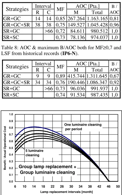
applying the AOC minimum criteria, that is, the more the maintenance is postponed the more economic it would result, however, the relation B/COA is null due to the fact that PFL is very low in this case. Nevertheless, for the criteria B/AOC maximum the curve presents an inflection point for a 14 months period of lamp replacement and luminaire cleaning (see fig. 5), but under this criteria the remaining policies present a greater
ratio B/AOC, being SR+GR the most convenient
from this point of view. It is interesting to point out that under this last policy there will be a coexistence of new lamps with the old depreciated ones still working, but with an average FM acceptable in theory. Similar conclusions, but with greater AOC and shorter replacement and cleaning periods, can be reached by using the survival curves with historical data (see Table 8).
In Fig. 6 is presented the case for SM+LM+SC
where the replacement and cleaning periods are the same for both criteria.
If luminaires IP2 are used (cost per light- point
163.000 Pta) the policies SR+GC and SR+SC
would not be the more indicated, because FM<0.7 giving illuminance values not acceptable, being
instead SR+GR+GC the most convenient for the
criteria B/AOC maximum.
Table 6: Minimum Annual Operation Costs and Benefit/AOC for MF ≥ 0,7 (luminaire IP6).
Interval AOC [Pta.]
Strategies R C MF M Total AOCB /
GR+GC 65 65 0,70 57.565 953.465 0 GR+GC+SR 38 38 0,75 149.527 1.045.428 0,96 SR+GC >66 0,72 84.611 980.512 1,0 SR+SC 0,73 78.136 974.037 1,0 R: Lamp replacement period [month], C: Luminaire cleaning period [month], M: Maintenance annual cost
Capital amortisation period: 15 years
Typical annual lamp operation time: 4270hs/year Actual annual lamp operation time: 4270hs/year Energy cost: 15 Pta/ kWh
PFLmin: 2% , PFLmax: 20% , PFL: 2% Costs per luminaire:
Labour group lamp replacement: 3.410 Pta. Labour group luminaire cleaning: 3.410 Pta.
Labour group lamp replacement & luminaire cleaning: 4.488 Pta.
Labour spot lamp replacement: 6.732 Pta.
Labour spot lamp replacement & simultaneous cleaning: 8.976 Pta.
SR+GC >66 0,72 84.611 980.512 1,0 SR+SC 0,73 78.136 974.037 1,0 Table 8: AOC & maximum B/AOC both for MF≥0,7 and LSF from historical records (IP6-N).
Interval AOC [Pta.]
Strategies R C MF M Total AOCB /
GR+GC 9 9 0,89 415.744 1.311.645 0,67 GR+GC+SR 34 34 0,76 190.446 1.086.347 0,92 SR+GC >66 0,73 96.036 991.937 1,0 SR+SC 0,74 91.534 987.435 1,0
Figure 5: B/AOC with GR+GC for example data.
Figure 6: B/AOC with SR+GR+GC for example data.
Table 9: Minimum AOC & B/AOC both for MF ≥ 0,7 and luminaire IP2-N
Interval AOC [Pta.]
Strategies R C MF M Total AOCB /
GR+GC 23 4,6 0,70 369.062 1.217.214 0,64 GR+GC+SR 23 4,6 0,70 391.230 1.239.383 0,80 SR+GC 6 0,60 264.411 1.112.563 0,64 SR+SC 0,47 78.136 926.288 0.36
SR+GC 6 0,60 264.411 1.112.563 0,64 SR+SC 0,47 78.136 926.288 0.36
4. CONCLUSIONS
The relationship Benefit/annual operational cost can be used as a decision criteria to establish the maintenance policy, lamp replacement period and cleaning frequency. In spite of the fact that benefit quantification can be discussed, nevertheless its use allows a more complete judgement of the situation. The optimisation procedure according to maximum B/AOC and minimum AOC criteria differ in some cases only quantitatively, but in others it can gide to different conclusions.
The inclusion of actual control parameters can affect the results allowing a continue evaluation process that could useful as a tool to incentive the efficient social use. The study continues at the present time in that direction.
AUTHORS
# Universidad Nacional de Tucumán, Instituto de
Luminotecnia Luz y Visión, Av. Independencia 1800 (4000) Tucumán, Argentina.
Fax:+34 93 3340255 Email: [email protected]
* Universitat Politècnica de Catalunya, Depto.
Projectes de L’Enginyeria, ETSEIB, Av. Diagonal 647, 08028 Barcelona, Spain
ACKNOWLEDGEMENTS
The authors with to thank to S.E.C.E. and M.O.S.E.C.A. Lighting maintenance Co. from Barcelona , to the students from the course Proyectos de la UPC and to the municipalities lighting managers, for their participation on the lighting surveys and data collection.
REFERENCES
[1] SAN MARTÍN R., MANZANO E.R.: A study
of indirect energy cost due to reduced urban
lighting maintenance, Proccedings CIBSE National
Lighting Conference, pag. 219 a 223, UK, 1998. [2] Universitat Politècnica de Catalunya: Encuestas sobre Gestión del Alumbrado en Ayuntamientos de Cataluña, España, en colaboración con los alumnos de la asignatura Proyectos, 1997-1998.
[3] MARSDEN A.M.: The economics of lighting
maintenance, Lighting Research &Tecnology, 25,
pag.:125-112. UK, 1993.
[4] British standard: BS 5489 Road Lighting, Part 1, 1992.
KEYWORDS
Urban lighting, Maintenance Group lamp replacement +
Group luminaire cleaning
0.0 0.1 0.2 0.3 0.4 0.5 0.6 0.7 0.8 0.9 1.0
6 10 14 18 22 26 30 34 38 42 46 50
Lamp replacement intervals [month]
Benefit / Anual Operational Cost
One luminaire cleaning per period
5 luminaire cleaning
Group lamp replacement + Group luminaire cleaning + Spot lamp
replacement 0.0 0.1 0.2 0.3 0.4 0.5 0.6 0.7 0.8 0.9 1.0
6 10 14 18 22 26 30 34 38 42 46 50
Lamp replacement intervals [month] one cleaning per period
5 cleanings per period
DUE TO REDUCED URBAN LIGHTING MAINTENANCE
San Martín, R. † / Manzano E.R ‡
† Universitat Politecnica de Catalunya, Depto. Projectes de L’Enginyeria, ETSEIB, Av. Diagonal 647, 08028 Barcelona, Spain.
‡ Universidad Nacional de Tucumán, Inst. de Luminotecnia Luz y Visión, Av. Independencia 1800, 4000 Tucumán, Argentina, Fax:+ 34 3 334 02 55, Email: [email protected]
1. INTRODUCTION
Urban lighting installations provide a service that is frequently not appreciated until lack is experimented. The opposite, a diminishing lumen output with time (depreciation), is hardly ever perceived. Consequently, lighting facilities require attention during operation in order to: guarantee a correct performance, reduce deterioration and adapt according to urban and technological evolution. Care must begin in the design stage and continue during all its useful life.
The current situation of lighting management and maintenance, when is accomplished, is mainly based on empirical criteria or acquired habits. Experience shows that a high percentage of lighting systems could be found presenting from mild deficiencies up to severe failure because of a lack in optimisation and planning of management and maintenance.
At the present time a project is being carried out at the Universitat Politecnica de Catalunya, in order to study and analyse the management and maintenance lighting problems of under a general cost / benefits approach. In a first stage evaluations of actual costs from the lack of maintenance in urban lighting systems are necessary to establish the weight of the different aspects involve and also as arguments to motivate right applications and the exploration of possible improvements in the practices of procedures.
2. APPROACH
While analysing the cost/benefit relationship that a urban lighting installation produces it is useful to identify the most relevant aspects, their relative importance and the method of evaluating them.
Urban lighting is a service to the citizen that must evolve according to the population growth and needs, changes in the electrical energy tariff rate, and new lighting technological developments. Moreover, during operation lighting facilities are depreciated. This requires a permanent care in order to prevent any reduction in the quality of the service.
Adequate lighting management permits considering all the involved aspects. It is also the best tool to achieve a rational energy consumption considering simultaneously the lighting systems efficiency.
policy, (spot, bulk, etc.) and administration costs (supervision, control etc.). Lack of an adequate maintenance policy, has a direct influence on costs because it reduces the maintenance operations cost, etc. Moreover it generates other indirect cost, usually overlooked, related to reducing the lighting system lifetime because the same investment must be amortised in a shorter period. Reducing lifetime from 20 to 12 years, with a financial interest of the 8%, makes an increase in the annual amortisation equivalent to 30%.
The natural gradual reduction of the lighting systems output, added to a reduction of the maintenance, has the consequence of increasing in energy consumption, wasting money, and reducing lifetime in components. This phenomenon, usually underestimated, can be the result of:
• lighting system operation out of the necessary schedules
• reactive power comsumption, due to lack of maintenance in the capacitors.
• improper tariff contract with the energy supplying company.
• poor energy supplying quality mainly caused by voltage supply variation.
• sporadic losses difficult to evaluate.
In order to evaluate the weight of each aspect mentioned above, different real cases were analysed.
2.1.1 CASE STUDY
From different areas of Barcelona a data survey of the urban lighting service was fulfilled during the period ranging from 1991 to 1996 and now studied in the light of analysing the increase in costs produced by lack of maintenance in order to establish limits and trends of the most relevant factors involved. By operation of the lighting system out of schedule: the increase in energy consumption can reach 25 to
30% [1] (table 1). The main cause of these high percentages was lack of maintenance associated with the use of photo-cell controls that require greater care. This conclusions are reinforced by comparison with other results arising from situations [2] in which a good maintenance policy was carried out and in where two sort of switch controls were available. The photo-cell control produced an average operation time (Toaverage) in excess of +11.4 min. which represents 1.6% of the energy consumption increase, while lighting systems fitted with programmable astronomical clocks† produced a Toaverage = +2,6 min., with a energy consumption increase of 0,4%.
Reactive power comsumption. This factor has in Spain a charge in tariff if the power factor cosϕ is < 0.9,
otherwise, a discount is applied, its percentage being calculated by means of: Kr(%)i = cos i172 21
ϕ − (1)
where Kr(%)i : percentage value to apply to the basic billing of the customer (i), as a discount if it is negative, or as a charge if its positive (capacity loads have charge).


![Figure 3: Variation of lighting network voltage [6] over a 24 h period. In bracket lines ±7% of 220V supply voltage is indicated.](https://thumb-us.123doks.com/thumbv2/123dok_es/5306629.98274/30.595.98.292.109.305/figure-variation-lighting-network-voltage-bracket-voltage-indicated.webp)