Digital Object Identifier (DOI) 10.1007/s002110000247
Numerische
Mathematik
A new approach for the optimal distribution
of assemblies in a nuclear reactor
Gr´egoire Allaire1,2, Carlos Castro1,3
1 CEA Saclay, DRN/DMT/SERMA, 91191 Gif-sur-Yvette, France
2 Laboratoire d’Analyse Num´erique, Universit´e Paris 6, 75252 Paris Cedex 5, France 3 Departamento de Matematica Aplicada, Universidad Complutense, 28040 Madrid, Spain
Received January 13, 2000 / Published online February 5, 2001 – cSpringer-Verlag 2001
Summary. The aim of this paper is to propose a new approach for optimiz-ing the position of fuel assemblies in a nuclear reactor core. This is a control problem for the neutronic diffusion equation where the control acts on the coefficients of the equation. The goal is to minimize the power peak (i.e. the neutron flux must be as spatially uniform as possible) and maximize the reactivity (i.e. the efficiency of the reactor measured by the inverse of the first eigenvalue). Although this is truly a discrete optimization problem, our strategy is to embed it in a continuous one which is solved by the homoge-nization method. Then, the homogenized continuous solution is numerically projected on a discrete admissible distribution of assemblies.
Mathematics Subject Classification (1991): 65K10; 65N99
1. Introduction
This paper is concerned with an optimal design problem in nuclear reactor cores: the so-called optimal fuel re-loading problem. In most reactor cores, the nuclear fuel is made of a few hundreds of so-called assemblies, period-ically distributed in a cross-section of the core (see Fig. 1). Each assembly is a very heterogeneous medium composed by a regular array of fuel pins (mainly made of uranium) and control rods immersed in water. During the fission process, the fissile isotope of uranium is consumed and other prod-ucts appear. This so-called depletion process progressively decreases the efficiency of the nuclear fuel. Therefore, it must be changed periodically by
fresh one (such a period, also called a cycle, is about a few months). How-ever, the fuel depletion is not spatially uniform in the core. This has two consequences: first, only part of the old assemblies (typically one fourth) are removed at the end of each cycle, second, it is not desirable to put the new assemblies exactly at the location of the removed ones. In order to maintain the maximal performance of the reactor, it is rather preferable to optimize the position of each type of assemblies. In other words, the fuel re-loading process not only consists in replacing the used assemblies by fresh ones but also in a rearrangement of all the assemblies in the core to make the most efficient use of the nuclear fuel. As such, it is a discrete optimization problem, but the large number of assemblies make it highly non-trivial since the computation of all possible combinations to find the best one is out of reach. For more details on this problem, we refer e.g. to [6, 9, 12].
In order to give a precise mathematical statement of this optimization problem, we now describe the state equation that models the fission process in the nuclear reactor and allows to quantify the efficiency of the assem-blies distribution. The power distribution in a nuclear reactor core is usually obtained by solving an eigenvalue problem for a diffusion equation. For simplicity, in this paper we content ourselves with the one energy group diffusion equation (multiple energy groups diffusion will be considered in a next paper [2]). In a steady-state regime, this problem gives the balance between neutrons produced by fission and neutrons absorbed or diffused by the medium. Denoting byΩ the radial section of the core (Ω ⊂ R2 is a bounded open set), our state equation is
−div (D(x)∇u(x)) +Σ(x)u(x) =λσ(x)u(x), x∈Ω, u(x) = 0, x∈∂Ω,
(1)
where the unknowns are the neutronic fluxu(i.e. the density of neutrons) and the eigenvalueλ= 1/keff (keffis the criticality parameter which gives the ratio between produced and consumed neutrons). More precisely,λis the first eigenvalue anduthe first eigenvector of (1), which is the only one to have a physical meaning since it is positive. The diffusion coefficient
gives only the spatial distribution of the neutron flux (which in turn yields the power distribution) but not its intensity since an eigenvector is defined up to a multiplicative constant.
We can now describe the objective function of the fuel re-loading op-timization problem. As already said, a reactor can produce energy if its criticality eigenvalueλis equal to or smaller than 1. However, as time goes by, the fuel depletion has a tendency to increase this eigenvalue. Therefore, at the beginning of a cycle it is highly desirable to have the smallest possible value ofλ(or criticality reserve), ensuring that the reactor will be working for the longest possible time. Minimizing the eigenvalueλmay cause un-usual oscillations in the profile of the first eigenvectoru(the neutron flux), and produce a highly non-uniform power distribution in the core (which is proportional toσu). For efficiency and safety reasons, it is rather an undesir-able feature. Indeed, at peak points of the power distribution, the surrounding flow of water could be unable to cool down the fuel pins, yielding a strong increase of the temperature that may eventually cause damage in the as-sembly. A major issue for safety is thus to have the most uniform power distribution in the core. This can be enforced by minimizing the maximal value ofσu(the so-called peak power point). Such a criterion is non differ-entiable, and we approximate it by minimizing instead theLr(Ω)norm of
σuwith1 < r <+∞. Since uis defined up to a multiplicative constant, we take care of normalizing thisLr(Ω)norm by theL1(Ω)norm. Finally, introducing a positive Lagrange multiplier≥0, our objective function is
min
λ+(MM(|σu(σu|r)))1/r
,
(2)
whereMdenotes the average operator inΩ
M(f) = |Ω1|
Ωf(x)dx.
(3)
For simplicity, we outrageously simplified the constraints and requirements used in practice for fuel re-loading optimization. In particular, we optimize the assemblies distribution just for one cycle, regardless of what may happen afterwards, and we do not take into account the cost of permuting assemblies. We also do not try to minimize the production of undesirable isotopes or species in the fission process. For more informations on the actual constraints and objectives, we refer e.g. to [12].
Fig. 1. A discrete configuration of two types of assemblies in a 900 Mw PWR nuclear reactor
core (having 157 assemblies)
physical characteristics (D, Σ, σ) due to their different past time in the core (their so-called burnup). Typical values ofI that we shall deal with in this paper are I = 2 or 4 (the case I = 2 is much simpler but not realistic, whileI = 4is typical and not much easier than anyI ≥ 3). For simplicity, we assume that all assemblies of the same type are identical, and that the coefficients (D, Σ, σ) are constant inside one assembly (i.e. it is homogeneous). Of course, the proportions of each type of assemblies are given. We make no special assumptions on the ordering of the physical properties of the assemblies, although physically speaking the freshest fuel produce the smallest criticity eigenvalueλ. Finally, since all assemblies have the same size, the coreΩcontains a finite number of them (see Fig. 1). Thus,
Uadis a finite set of all possible permutations of these assemblies.
Fig. 2. A continuous configuration of two types of assemblies in a 900 Mw PWR nuclear
reactor core
that it will lead to a nearly optimal admissible configuration of assemblies. Transforming an admissible configuration into a continuous one is obtained through a numerical method of penalization. This second step is therefore purely based on numerical heuristics and has no firm theoretical ground. On the contrary, we perform a detailed mathematical analysis of the first step. It turns out that the continuous optimization problem is ill-posed in the sense that it does not admit a solution in the space of all possible continu-ous distributions of theI materials. The reason for this is that minimizing sequences of almost optimal configurations have a tendency to exhibit very fine mixture of theI components. On a macroscopic scale these mixtures are composite materials having effective properties different from that of its phase constituents. Their effective or averaged cross sections and diffusion tensors are found by using the homogenization theory. To make this problem well-posed, one must enlarge the space of admissible designs by allowing for composite materials obtained by mixing microscopically theI different fuels. We then obtain the existence of a composite optimal configuration, as well as very efficient numerical algorithm for computing them.
rather a pre-processor, since its final output could still be refined by these methods.
Finally, we conclude this introduction by a brief description of the con-tent of this paper. Although our goal is to address the case ofI >2types of assemblies, for simplicity our exposition starts with the easier caseI = 2. In Sect. 2, a mathematical setting is introduced for the original continuous problem. Section 3 is devoted to its relaxation, and Sect. 4 deals with op-timality conditions. Eventually Sect. 5 generalizes the previous results for more than two type of assemblies. Numerical results are presented in Sect. 6.
2. Setting of the problem
We first recall that the state equation of our optimization problem is the spectral equation for the one energy group diffusion model. Denoting byΩ a bounded open set inR2, it reads
−div (D(x)∇u(x)) +Σ(x)u(x) =λσ(x)u(x), x∈Ω, u(x) = 0, x∈∂Ω,
(4)
where(λ, u)is the first eigenvalue and eigenvector. The coefficients in (4) are assumed to be measurable and bounded (but not necessarily smooth), i.e.D, Σ, σ∈L∞(Ω). Furthermore, we assume that, almost everywhere in
Ω, they satisfy
Σ(x)≥0, σ(x)≥σ0 >0, D(x)≥d0 >0.
Under these assumptions, it is well known that (4) admits a unique solution in the sense given by the following result (see e.g. [20]).
Theorem 2.1 There exists a countable infinite number of eigenvalues for (4), that we label by increasing order as(λi)i≥1, and corresponding eigen-vectors (ui)i≥1 ∈ H01(Ω). Furthermore, the first eigenvalue λ1 (i.e. the smallest one) is positive and simple, and its eigenvector is the only one that can be chosen to be positive inΩ.
Remark 2.2 The only solution of (4) which has a physical meaning is the first eigenvalue and eigenvector(λ1, u1)sinceu1is the only eigenvector to be positive (a necessary feature for a density function). From now on, we drop the subscript 1, and denote by(λ, u) = (λ1, u1)the solution of (4). Of course,uis unique only up to a multiplicative constant.
i.e. we do not require that each type of materialj= 1,2fit into assemblies, but it may rather fill the domainΩ in any possible shape. In other words, denoting byΩj the part ofΩoccupied by materialj, there is no restrictions on(Ω1, Ω2)except the obvious ones
Ω1∩Ω2 = 0, Ω1∪Ω2 =Ω, |Ωj|=γj, j = 1,2.
(5)
Introducing the characteristic functions(χ1, χ2)of these subsets(Ω1, Ω2) (i.e.χj(x) = 1ifx ∈Ωj andχj(x) = 0ifx∈\Ωj), the coefficients of (4) are given by
D(x) =d1χ
1(x) +d2χ2(x),
Σ(x) =Σ1χ1(x) +Σ2χ2(x),
σ(x) =σ1χ
1(x) +σ2χ2(x). (6)
Sinceχ1+χ2 = 1, a single characteristic functionχ1 = χdefines com-pletely the distribution of the two fuel types. Therefore, the space of admis-sible configurations can now be defined in a very simple way by
Uad =
χ∈L∞(Ω;{0,1})such that
Ωχ(x)dx=γ1
.
(7)
Our fuel re-load optimization problem is to find a minimizer of
min
χ∈UadJ(χ) = λ+
(M(|σu|r))1/r
M(σu)
,
(8)
where(λ, u)is the solution of (4),Mis the average operator inΩdefined by (3),1< r <+∞, and the coefficients of (4) are given by (6).
To solve this optimization problem we can try the direct method of the calculus of variations. It amounts to proceed in the following order
1. We prove that minimizing sequences are relatively compact for a suitable topology.
2. We prove a lower semicontinuous result for the objective function, which yields that it attains its minimum.
3. We differentiate the cost function to obtain optimality conditions. As remarked by [18], two main problems arise when we try to carry out this process for (8). First, the set Uad is not closed in the topologies for which minimizing sequences are compact. This means that, in general, minimizing sequences can converge to limits outside from Uad, i.e. they are not characteristic functions. In this case there is no minimizer of (8) in
To overcome these two obstacles, one can use the so-called relaxation procedure (see e.g. [5, 7]). It amounts to extend the original space of admis-sible solutions into a space of generalized, or relaxed, admisadmis-sible solutions, denoted byUad∗ , as well as the objective functionJ that becomes a relaxed objective functionJ∗. This extension is built to guarantee the existence of an optimal relaxed solution, but it should not be too ”large” in order to keep track of the behavior of minimizing sequences for the original problem. In other words, relaxing a problem does not change its physical significance. More precisely, a relaxed formulation must satisfy the following conditions 1. Uad⊂ Uad∗ and the relaxed cost function coincides with the original one
overUad,
2. there exists at least one minimizer of the relaxed problem, and the min-imal values of the original and relaxed objective functions are equal, 3. any minimizer of the relaxed problem is attained by a minimizing
se-quence of the original problem,
4. any minimizing sequence of the original problem converges to a mini-mizer of the relaxed problem.
In the next section we introduce such a relaxation for our problem using homogenization.
3. The relaxed problem
In this section we introduce a relaxed problem associated to (8). We follow the homogenization method introduced in [18].
The set of characteristic functions is bounded inL∞(Ω)and therefore relatively compact for the weak * convergence. Thus, from any sequence (χn)n≥1 inUad, we can extract a subsequence, still denotedχn, such that it converges weakly * inL∞(Ω) to a limitθ(x). Since the convergence is weak and not strong,θis usually not anymore a characteristic function but a density, i.e.θ(x)may take its values in the full range[0,1]. Defining the corresponding coefficients
Dn(x) =χn(x)d1+ (1−χn(x))d2,
Σn(x) =χn(x)Σ1+ (1−χn(x))Σ2,
σn(x) =χn(x)σ1+ (1−χn(x))σ2,
the state equation is rewritten
−div (Dn∇un) +Σnun=λnσnun, inΩ,
un= 0, on∂Ω,
(9)
G-convergence, see e.g. [10, 18]), which states that, up to a subsequence, the limit of (9) is the following homogenized problem
−div (D∗∇u(x)) +Σu(x) =λσu(x), x∈Ω,
u(x) = 0, x∈∂Ω,
(10)
where(λ, u) are the first eigenvalue and normalized eigenvector, and the homogenized coefficients are defined by
Σ(x) =θ(x)Σ1+ (1−θ(x))Σ2, σ(x) =θ(x)σ1+ (1−θ(x))σ2,
and D∗ is the H-limit (i.e. the limit in the sense of homogenization) of the sequenceDn = χnd1 + (1−χn)d2. This H-convergence has to be understood in the following sense
lim
n→∞λn=λ,
un uinH01(Ω)weakly. (11)
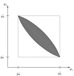
It turns out that, although the homogenized cross sectionsΣ, σare uniquely defined by the limit densityθ, the homogenized diffusion coefficientD∗ is not explicitly characterized byθ. Indeed, depending on the geometry of the mixture represented by the sequenceχn,D∗may be any symmetric positive definite matrix in a setGθ. This set of all possible homogenized diffusion tensors associated to the density θhas been characterized in [13, 18]. We assume, with no loss of generality, that0< d1 ≤d2. At any pointx∈Ω,
D∗(x)is any symmetric matrix with eigenvalues(µ1(x), µ2(x))satisfying
(see Fig. 3)
1
µ1−d1 + 1
µ2−d1 ≤ 1
µ−θ −d1 + 1
µ+θ −d1, (12)
1
d2−µ1 +d2−1 µ2 ≤ d2−1µ−
θ +
1
d2−µ+
θ .
(13)
where µ+θ and µ−θ are the arithmetic and harmonic means of the phase diffusion coefficients
µ+
θ =θd1+ (1−θ)d2,
µ−
θ = θ/d1+ (11−θ)/d2.
(14)
One can easily check that (12) implies thatµ−θ ≤µi≤µ+θ fori= 1,2. Since the homogenized state equation (10) depends on two design pa-rameters, namelyθandD∗, the set of generalized admissible configurations
U∗
admust be the set of such couples, namely
U∗
ad =
(θ, D∗)∈L∞(Ω)such that0≤θ≤1, D∗∈G
θ,
Ωθ=γ1
,
+ µ
θ + µ θ
− µ θ
− µ
θ µ
1 2
µ
Fig. 3. SetGθof all homogenized diffusion tensors
where the constraints on(θ, D∗)are pointwise inΩ. Remark that we have
Uad ⊂ Uad∗ if we associate to each characteristic functionχ∈ Uada diffusion tensorD=d1χ+d2(1−χ). By Rellich theorem, the sequenceun, which converges weakly touinH01(Ω), converges strongly touinLr(Ω)for any 1 ≤ r < +∞ in two space dimensions (and for any1 ≤ r < 6in three dimensions). Sinceχnconverges weakly * toθinL∞(Ω), we deduce that (σn)rconverges weakly * toθ(σ1)r+(1−θ)(σ2)rinL∞(Ω), and therefore
lim
n→∞
Ωσn(x)un(x)dx=
Ωσ(x)u(x)dx,
while
lim
n→∞
Ω|σ(x)un(x)|
rdx=
Ω|s(x)u(x)|
rdx,
withsbeing usually different fromσ
s(x) =θ(x)(σ1)r+ (1−θ(x))(σ2)r1/r.
Thus, combined with (11) we obtain lim
n→∞J(χn) =J
∗(θ, D∗),
andJ∗ is a relaxed objective function defined by
J∗(θ, D∗) = λ+(M(|su|r))1/r
M(σu)
,
(16)
where (λ, u) is the first eigenvalue and eigenvector of (10) (remark that Theorem 2.1 also applies to (10)). Our relaxed problem is finally to minimize
J∗overU∗
min (θ,D∗)∈U∗
ad
J∗(θ, D∗).
(17)
We can now state the main result of relaxation.
Theorem 3.1 Assume that 1 ≤ r < +∞ in two space dimensions, and 1< r <6in three dimensions. The relaxation of the original optimization problem (8) is (16) in the sense that
1. there exists at least one minimizer inUad∗ ofJ∗,
2. any minimizer(θ, D∗)of the relaxed problem is attained by a minimizing sequenceχnof the original problem in the sense that
χn θweakly * inL∞(Ω),
Dn=χnd1+ (1−χn)d2 H-converges toD∗,
and
inf
χ∈UadJ(χ) =(θ,Dmin∗)∈Uad∗ J
∗(θ, D∗),
3. any minimizing sequence χn of the original problem converges to a minimizer(θ, D∗)of the relaxed problem.
Proof. This proof is an adaptation of that in [18]. It is a simple consequence of the convergence result (11). Indeed, ifχnis a minimizing sequence for
J, (11) implies that χn converges to θ∞ and J(χn) converges, up to a subsequence, toJ∗(θ∞, D∗∞)which is therefore equal tominχ∈UadJ(χ). Since any(θ, D∗)is attained by a sequenceχn(not necessarily minimizing), we deduce that(θ∞, D∞∗ )is a minimizer ofJ∗. This finishes the proof of Theorem 3.1.
4. Optimality conditions
One advantage of the relaxed formulation is that it allows to derive optimality conditions that are of both theoretical and numerical interest. The results of this section are a variation of those in [18]. The relaxed cost functionJ∗ is defined by
J∗(θ, D∗) =λ+(M(|su|r))1/r
M(σu) .
(18)
withM(f) =|Ω|−1Ωf(x)dx. By theorem 2.1 the first eigenvalueλand the first normalized eigenvectoruare simple : therefore, they are Gˆateaux-differentiable, as well asJ∗, with respect to(θ, D∗)in the admissible set
Uad∗ =
(θ, D∗)∈L∞(Ω)such that0≤θ≤1,
Ωθ=γ1, D
∗ ∈G
θ
.
If(δθ, δD∗)is an admissible increment inUad∗ , the derivative ofJ∗is
δJ∗=δλ+(M(|su|r))(1−r)/r
M(σu) M
(su)r−1(sδu+uδs)
−(M(|su|r))1/r
(M(σu))2 M(σδu+uδσ), (20)
wherersr−1δs= ((σ1)r−(σ2)r)δθ,δσ = (σ1−σ2)δθ,δλis the increment in the first eigenvalue, andδuis the increment in the first eigenvector solution of (10). To computeδλ, we first remark that multiplying equation (10) by a test functionv ∈H01(Ω)yields
λ=
Ω
D∗∇u· ∇v+Σuvdx
Ωσuvdx
.
(21)
Thus, differentiating (21) gives after some easy algebra
δλ=
ΩδD∗∇u· ∇udx+
Ω|u|2δΣdx
Ωσ|u|2dx −λ
Ω|u|2δσdx
Ωσ|u|2dx .
(22)
On the other hand, differentiating (10) shows thatδuis the unique solution inH01(Ω)of
−div (D∗∇(δu)) +Σδu−λσδu= div (δD∗∇u)−δΣu
+(λδσ+σδλ)u inΩ,
δu= 0 on∂Ω. (23)
Remark that the right hand side of (23) is orthogonal to the first eigenvector
u which implies that it admits a solution, unique up to the addition of a multiple ofu.
As usual, to eliminateδuan adjoint stateqis introduced. It is defined as the unique solution inH01(Ω)of
−div (D∗∇q) +Σq−λσq
= (M(|suM|r(σu))(1)−r)/rsrur−1
|Ω| −(M(|su|
r))1/r
(M(σu))2 |Ωσ| inΩ, q= 0 on∂Ω.
(24)
Remark that the right hand side of (24) is orthogonal tou which implies that it admits a solution, unique up to a multiple ofu. Then, multiplying equation (24) byδuand equation (23) byqleads to
(M(|su|r))(1−r)/r
M(σu)
1
|Ω|
Ωs
rur−1δudx−(M(|su|r))1/r
(M(σu))2 1 |Ω| Ωσδudx =− ΩδD
∗∇u· ∇qdx−
Ω
δΣ−λδσ−σδλuqdx.
Thus
δJ∗(θ, D∗) =δλ+ (M(|su|r))(1−r)/r
M(σu)
1
|Ω|
Ωu
rsr−1δsdx
−(M(|su|r))1/r
(M(σu))2 1
|Ω|
Ωuδσdx
−
ΩδD
∗∇u· ∇qdx−
Ω
δΣ−λδσ−σδλuqdx.
Introducing a combination functionp∈H01(Ω)defined by
p= +
Ωσuqdx
Ωσ|u|2dx u−q,
(26)
the derivative ofJ∗becomes
δJ∗(θ, D∗) =
ΩδD
∗∇u· ∇pdx+
Ω
δΣ−λδσupdx
+(M(|Msu|(rσu))(1)−r)/r|Ω1|
Ωu
rsr−1δsdx
−(M(|su|r))1/r
(M(σu))2 1
|Ω|
Ωuδσdx,
(27)
whereδσ = (σ1−σ2)δθ,δΣ = (Σ1−Σ2)δθ, andrsr−1δs= ((σ1)r− (σ2)r)δθ.
Lemma 4.1 A necessary condition for(θ, D∗)to be a minimizer ofJ∗ in
U∗
adis
δJ∗(θ, D∗)≥0 (28)
for any admissible increment(δθ, δD∗).
According to the structure ofUad∗ , the minimization process can be carried out in two steps: firstly inD∗and secondly inθ. In other words,
min (θ,D∗)∈U∗
ad
J∗(θ, D∗) = min
0≤θ≤1Dmin∗∈GθJ
∗(θ, D∗).
(29)
Proposition 4.2 Whenδθ= 0, the optimality conditions becomes
δJ∗(θ, D∗) =
ΩδD
∗∇u· ∇pdx≥0.
(30)
It implies that, outside the set where|∇u||∇p| = 0, an optimal diffusion tensorD∗satisfies
D∗∇u= 1
2(µ+θ +µ−θ)∇u−12(µ+θ −µ−θ)|∇|∇up||∇p,
D∗∇p=−1
2(µ+θ −µ−θ)|∇|∇pu||∇u+12(µ+θ +µ−θ)∇p.
(31)
Besides, defining an angleϕby∇u· ∇p=|∇u||∇p|cosϕ, we obtain
D∗∇u· ∇p=|∇u||∇p|µθ−cos2 ϕ2 −µ+θ sin2ϕ2.
(32)
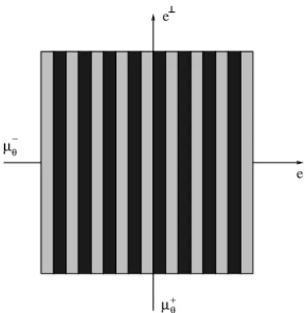
Remark 4.3 As a byproduct of Proposition 4.2, it turns out that, at the points where∇u /= 0and∇p /= 0, an optimal diffusion tensorD∗can always be found in the class of so-called simple laminates or layered materials (see the proof below). A careful investigation of the remaining points|∇u||∇p|= 0 shows that, everywhere, an optimalD∗can be found in the class of layered materials (this remarks is due to [18, 21]). A layered material is obtained by stacking slices of the two components 1 and 2 and computing its effective or homogenized properties (see Fig. 4). It turns out that there is an explicit formula for its homogenized tensorD∗which depends on the volume frac-tionθof phase 1 and on the unit directionewhich is normal to the slices or layers. In 2-D, in the basis(e,e⊥)it reads
D∗ = diagµ−θ, µ+θ, (33)
i.e. the diffusion is the harmonic average in the normal direction of the layers while it is the arithmetic average in the direction parallel to the layers.
Taking into account the optimal diffusion tensorD∗furnished by Propo-sition 4.2, we know vary the volume fractionθto obtain
Proposition 4.4 Defining a functionQ(x)by
Q(x) =|∇u||∇p|
dµ−θ dθ cos2
ϕ
2 −
dµ+θ dθ sin2
ϕ
2
+(Σ1−Σ2)−λ(σ1−σ2)up
+(M(|su|r))(1−r)/r
M(σu)
(σ1)r−(σ2)rur
r|Ω|
−(M(|su|r))1/r
(M(σu))2
(σ1−σ2)u
|Ω| ,
−
e e
µθ+
µθ
Fig. 4. A two-phase layered material
there exists a constantC0such that a minimizer(θ, D∗)forJ∗ satisfies
θ(x) = 0ifQ(x)< C0, 0≤θ(x)≤1ifQ(x) =C0,
θ(x) = 1ifQ(x)> C0, (35)
and reciprocally
Q(x)≤C0 ifθ(x) = 0,
Q(x) =C0 if0< θ(x)<1,
Q(x)≥C0 ifθ(x) = 1. (36)
Proof of Proposition 4.2. Takingδθ= 0implies thatδσ =δΣ =δs= 0, which in turn yields (30). It also implies that the variationδD∗stays inside the setGθ. It turns out thatGθis a convex set of symmetric matrices since it is defined as a convex set of eigenvalues (see [18]). Therefore,δD∗can be parallel to any straight line inGθ passing throughD∗. In other words, for anyC∗ ∈Gθ, we can choose
δD∗ =C∗−D∗.
Thus, (30) implies
ΩC
∗(x)∇u· ∇pdx≥
ΩD
∗(x)∇u· ∇pdx, ∀C∗ ∈G
θ.
(37)
Equation (37) implies that the optimal D∗(x) is at each point x ∈ Ω a minimizer ofC∗(x)∇u(x)· ∇p(x)over all matricesC∗(x)∈Gθ(x). This minimization problem has been solved in [18]. If∇uor∇pis equal to 0, any matrix is a minimizer. If∇u /= 0and∇p /= 0, then, upon defining two unit vectorse=∇u/|∇u|ande =∇p/|∇p|, any minimizerD∗satisfies
D∗e= 1
2(µ+θ +µ−θ)e−12(µ+θ −µ−θ)e
and
D∗e = 12(µ+θ +µ−θ)e−12(µ+θ −µ−θ)e.
(39)
Furthermore, a minimizer is necessarily a so-called rank-one laminate in the direction of(e+e) ife+e = 0/ , or in a direction orthogonal toeif
e+e = 0. This leads to the desired result.
Proof of Proposition 4.4. We now take an optimalD∗defined by Proposition 4.2. This implies thatδD∗is a function ofδθ. In particular, we have
δD∗∇u· ∇p=|∇u||∇p|dµ−θ
dθ cos2 ϕ
2 −
dµ+θ dθ sin2
ϕ
2
δθ,
(40)
whereϕis defined by (32). Introducing the functionQ(x), we obtain
δJ∗(θ, D∗) =
ΩQ(x)δθ(x)dx≥0,
which, upon taking into account the volume constraint Ωδθ(x)dx = 0, yields the desired result (the constant C0 is the corresponding Lagrange multiplier).
Remark 4.5 The above optimality conditions are at the root of a numerical algorithm which is described in Sect. 6.
5. Generalization to more types of assemblies
In this section, we keep the same model of one energy group diffusion equation (4) and of objective function (8), but we change the definition of admissible configurations Uad by allowing for more than two types of assemblies. LetIdenotes the number of different types of assemblies. Each typei, with 1 ≤ i ≤ I, is characterized by a diffusion coefficientdi and cross sectionsσi, Σi, and occupies a given volumeγiin the domainΩwith
I
i=1
γi =|Ω|, γi≥0.
We denote byχi(x)the characteristic function of that part ofΩ occupied by assemblyi. Clearly, it satisfies
I
i=1
χi(x) = 1, χi(x)χj(x) = 0ifi /=j,
Ωχi(x)dx=γi.
The coefficients of (4) are now given by
D(x) =Ii=1diχ
i(x),
Σ(x) =Ii=1Σiχi(x),
σ(x) =Ii=1σiχ
i(x).
(42)
The space of admissible configurations is therefore defined as
Uad ={(χi)1≤i≤I ∈L∞(Ω;{0,1})satisfying (41)}. (43)
As in the case of two type of assemblies, the minimization of (8) is not well-posed inUad, i.e. there exist no minimizers. As before we introduce a relaxation of this problem by considering generalized designs in a space
U∗
ad.
The relaxation is built by using the homogenization theory (see e.g. [10, 18]) which works equally well for a mixture of any numberI of compo-nents. The same arguments of H-convergence leads to the homogenized state equation
−div (D∗∇u(x)) +Σu(x) =λσu(x), x∈Ω,
u(x) = 0, x∈∂Ω,
(44)
where(λ, u)are the first eigenvalue and eigenvector, and the homogenized coefficients are defined by
Σ(x) =I
i=1
θi(x)Σi, σ(x) = I
i=1
θi(x)σi,
where eachθiis a density function which is the weak * limit inL∞(Ω; [0,1]) of a sequence of characteristic functions(χin)n≥1of the subdomain occupied by assemblyi. These proportion functions satisfy
I
i=1
θi(x) = 1,
Ωθi(x)dx=γi, 0≤θi(x)≤1.
(45)
The homogenized diffusion tensorD∗(x)is theH-limit (i.e. the limit in the sense of homogenization) of the sequenceDn =Ii=1χindi. The relaxed objective function is defined by
J∗(θ, D∗) = λ+(M(|su|r))1/r
M(σu)
,
(46)
where(λ, u)is the solution of (44). The set of generalized admissible con-figurations is defined by
U∗
ad={(θ1,· · ·, θI, D∗)∈L∞(Ω)satisfying (45), such thatD∗∈Gθ},
where the constraintD∗ ∈Gθholds almost everywhere inΩ, andGθis the set of all possible homogenized diffusion tensors associated to the family of proportionsθ= (θ1,· · ·, θI). Our relaxed problem is therefore to minimize
J∗overU∗
ad, i.e.
min (θ,D∗)∈U∗
ad
J∗(θ, D∗).
(48)
One can prove a relaxation result completely similar to Theorem 3.1 which states that (48) is the true relaxation of the original optimization problem. For the sake of brevity, we shall not dwell on this. Unfortunately, this relaxed formulation is not very useful since we do not know an algebraic charac-terization of the setGθ whenI ≥ 3, on the contrary of the previous case
I = 2. Nevertheless, as was first remarked by Raitum [21] (see also [22]), we do not need the full setGθfor our optimization problem. It turns out that optimal arrangements of the components can always be found in the smaller subset of simple laminates or layered materials (this was already the case whenI = 2, see Remark 4.3).
Let us explain this ”miracle” that allows to treat the caseI ≥3as the previous oneI = 2(a similar argument has already been given in [22]). We define a set Cθ of all symmetric matrices with eigenvalues bounded between the harmonic and arithmetic means, i.e.M ∈Cθif and only if its eigenvaluesµ1, µ2 satisfy
µ−θ ≤µi≤µ+θ, fori= 1,2, (49)
where
1
µ−θ =
I
i=1
θi
di andµ+θ = I
i=1
θidi.
(50)
A well-known result of homogenization (see e.g. [10, 18]) states thatGθ is included inCθ, i.e. any homogenized tensorD∗ ∈ Gθ satisfiesµ−θId ≤
D∗ ≤µ+
θIdin the sense of quadratic forms. This inclusion is also known to
be strict, i.e.Gθ =/ Cθ. We then introduce a larger set of admissible designs
Uadc ={(θ1,· · ·, θI, D∗)∈L∞(Ω)satisfying (45),
such thatD∗ ∈Cθ}. (51)
The setUadc has no physical meaning: its tensorsD∗are usually not ho-mogenized tensors corresponding to a fine mixture of the phase components. It is just a mathematical artefact. SinceUad∗ ⊂ Uadc , we have
min (θ,D∗)∈Uc
ad
J∗(θ, D∗)≤ min
(θ,D∗)∈U∗
ad
J∗(θ, D∗).
(52)
such thatθnconverges toθ∞inL∞(Ω; [0,1])weak *, andD∗nH-converges toD∗∞. Furthermore, by the properties ofH-convergence (see (11)), we have
lim
n→+∞J∗(θn, Dn∗) =J∗(θ∞, D∗∞).
The only thing to check is that(θ∞, D∗∞)does indeed belong toUadc . Another classical result of homogenization tells us that
D∗∞≤D+∗, (D∗∞)−1 ≤D+∗−1,
whereD∗+ (respectively(D−∗)−1) is the weak * limit ofDn∗ (respectively (D∗
n)−1) inL∞(Ω). SinceD∗n∈Cθit satisfies
D∗
n≤µ+θnId, (D∗n)
−1 ≤µ−
θn
−1
Id,
where both right hand sides of the inequalities are affine function ofθn, which implies that in the limit
D∗
∞≤µ+θ∞Id, (D∗∞)
−1 ≤µ−
θ∞
−1
Id,
i.e. D∞∗ ∈ Cθ∞ as desired. In other words, J∗ attains its minimum at (θ∞, D∞∗ ) in Uadc . As proved in the next theorem, the optimality
condi-tions inUadc furnish a minimizer inUad∗ . Therefore, it is sufficient to find minimizers inUadc for obtaining a particular minimizer inUad∗ , which yields a tractable relaxation for numerical computations.
Theorem 5.1 There exists at least one couple(θ∞, D∞∗ )∈ Uad∗ , such that
D∗
∞is the effective tensor of a layered material, which is a minimizer ofJ∗
both inUad∗ and inUadc .
Remark 5.2 A layered material is obtained by stacking slices of theI com-ponents. Its effective or homogenized propertiesD∗ can be computed ex-plicitly in terms of the proportionsθ= (θ1,· · ·, θI)and the unit directione which is normal to the slices or layers. In 2-D, in the basis(e,e⊥)it reads
D∗ = diagµ−θ, µ+θ, (53)
whereµ−θ andµ+θ are defined by (50).
solution of (26). SinceCθis a convex set, arguing as in Proposition 4.2, the optimal tensorD∗satisfies, outside the set where|∇u||∇p|= 0,
D∗∇u= 1
2(µ+θ +µ−θ)∇u−12(µ+θ −µ−θ)|∇|∇up||∇p,
D∗∇p=−1
2(µ+θ −µ−θ)|∇|∇pu||∇u+12(µ+θ +µ−θ)∇p,
(54)
and it is necessarily a layered material whose orientation is given in terms of the angle between∇uand∇p. Tartar [22] generalized the clever trick of [21], mentioned in Remark 4.3, to the case ofI > 2phases. It enables to prove that, even where|∇u||∇p| = 0, one can find an optimalD∗ which is a layered material. This shows that at least one optimal tensorD∗ inUadc corresponds to a layered material which implies that it belongs toUad∗ and is therefore optimal inUad∗ too. Let us show that, if(θ, D∗)is a minimizer, then there exists another minimizer(˜θ,D˜∗)with the same stateuand adjoint state
psuch thatD˜∗is a simple laminate. If∇u= 0, we can clearly takeθ˜=θ and replaceD∗by any simple laminateD˜∗: it does not changeualthough
pmay change. When∇p= 0, we are going to change bothθandD∗while keeping the same stateuand adjoint statep(a symmetric argument would also work in the case∇u= 0). Indeed, by Lemma 5.3 below, there existI families of proportions(θk)1≤k≤I with componentsθk = (θki)1≤i≤I such thatIi=1θki = 1,θik ≥0, the rank of this family isI −1, and there exist simple laminatesDk∈Gθk satisfyingD∗∇u=Dk∇ufor all1≤k≤I.
Denoting byωthe measurable subset ofΩwhere∇p= 0, we buildθ˜inω by partionningωin subsetsωkwhere it takes only the valueθk(depending on∇uandD∗∇u), which minimizes the ”restriction” of the cost function toω, while satisfying the volume constraints on each phase (this is possible since the rank of(θk)1≤k≤IisI−1). Similarly,D˜∗is defined as the simple laminateDkin eachωk. We have thus obtained another minimizer(˜θ,D˜∗) which is a simple laminate.
Lemma 5.3 LetBbe a symmetric matrix, with eigenvalues(µi)1≤i≤N sat-isfyingµ−θ ≤µi≤µ+θ. Leteandebe two vectors inRN such thate=Be. Then, we have
e−12(µ+θ +µ−θ)e ≤ 12(µ+θ −µ−θ)e.
(55)
Furthermore, there exist I families of proportions (θk)1≤k≤I, depending only oneande, with componentsθk = (θik)1≤i≤I such thatIi=1θik = 1 andθki ≥0, and there exist simple laminatesDk∈Gθk such that, for any
1≤k≤I,
Proof. By definition, the eigenvalues of(B−12(µθ++µ−θ)Id)belong to the interval[−12(µ+θ −µ−θ),21(µ+θ −µ−θ)]which implies (55). Fort∈ RI, let us introduce a functionf(t)defined by
f(t) = 14(µ+t −µ−t )2e2− e−1
2(µ+t +µ−t )e2
=−µ+
t e−e
·µ−
te−e
.
An easy computation shows that, for tk = (δik)1≤i≤I (corresponding to pure phasek),f(tk) = −e−dke2, whilef(θ) ≥ 0by virtue of (55). Sincef(t)is continuous, on each segment[θ, tk]there exists a pointθksuch thatf(θk) = 0,Ii=1θik = 1andθki ≥0. The collection(θk)1≤k≤Iis of rank I −1 iff(tk) < 0andf(θ) > 0(if this is not the case,B can be replaced by a pure phase or a simple laminate). For suchθkwe have from
f(θk) = 0
fk·gk= 0withfk= µ +
θke−e
µ+
θk−µ−θk
andgk = µ
−
θke−e
µ+
θk−µ−θk
.
Then, defining a rank-one laminateDk∈Gθkin the directionfkiffk= 0/ ,
or in any direction orthogonal togkiffk= 0, we have
Dkfk=µ−
θkfkandDkgk =µ+θkgk.
Sincee=fk−gkande=µ−θkfk−µ+θkgk, we thus deduce thatDke=e, as desired.
We now turn to the optimality conditions for the volume fractionsθi. Let us define an angleϕbetween∇uand∇pby
∇u· ∇p=|∇u||∇p|cosϕ,
(56)
whereuandpare solutions of (44) and (26) respectively. By taking the opti-mal layered materialD∗furnished by Theorem 5.1, the optimal proportions
θ= (θ1,· · ·, θI)satisfy the following optimality conditions
Proposition 5.4 For1≤i≤I, letQi(x)be functions defined by
Qi(x) =−|∇u||∇p|
∂µ−
θ
∂θi cos
2 ϕ 2 −
∂µ+θ ∂θi sin
2ϕ 2
+Σi−λσiup
+(M(|Msu|(rσu))(1)−r)/r(σri|)Ωru|r −(M(|su|r))1/r
(M(σu))2
There exist a functionC0(x)and constantsCisuch that a minimizer(θ, D∗) forJ∗satisfies
θi(x) = 0ifQi(x)−C0(x)< Ci, 0≤θi(x)≤1ifQi(x)−C0(x) =Ci,
θi(x) = 1ifQi(x)−C0(x)> Ci,
and reciprocally
Qi(x)−C0(x)≤Ciifθi(x) = 0,
Qi(x)−C0(x) =Ciif0< θi(x)<1,
Qi(x)−C0(x)≥Ciifθi(x) = 1.
The proof of Proposition 5.4 is completely similar to that of Proposition 4.4. In particular, taking the optimalD∗implies that
δJ∗ =
Ω I
i=1
Qi(x)δθi(x)dx≥0,
which, upon taking into account theIvolume constraintsΩδθi(x)dx= 0 and the pointwise constraintIi=1θi = 1, yields the desired result.
6. Numerical algorithms
This section is devoted to a gradient-type numerical algorithm for solving the proposed relaxed formulation of the re-loading optimization problem (in two space dimensions). It relies on our knowledge of the optimality conditions and, in particular, of the optimality of simply layered microstructures. By virtue of Remark 4.3, the optimal homogenized diffusion tensor D∗ can be chosen to be that of a layered material which is parametrized by two variables : the volume fractionsθ= (θ1,· · ·, θI)and a rotation angleα. We therefore work with the following class of diffusion tensors
D∗(θ, α) =cosα sinα
−sinαcosα µ
+
θ 0
0 µ−θ cossinαα−cossinαα
,
whereµ−θ andµ+θ are defined by (50). In other words, our objective function
J∗is now a function of the(I+ 1)scalar design variablesθandα, subject
to the constraints
I
i=1
θi(x) = 1, 0≤θi(x)≤1,
Ωθi(x)dx=γi.
The computation of the gradient ofJ∗with respect to(θ, α)is very similar to the derivation of the optimality conditions in Sect. 4. For an admissible increment(δθi, δ α), we find
δJ∗(θ, α) =
Ω
∂D∗
∂α ∇u· ∇p δ αdx+
I
i=1
ΩQi(x)δθidx,
whereQi(x), being very similar toQi(x), is defined by
Qi(x) = ∂µ−θ
∂θi
sin2α∂u∂x∂p∂x+ cos2α∂u∂y∂p∂y
+ cosαsinα
∂u ∂x ∂p ∂y+ ∂u ∂y ∂p ∂x +∂µ+θ ∂θi
cos2α∂u
∂x ∂p ∂x
+ sin2α∂u∂y∂p∂y −cosαsinα
∂u ∂x ∂p ∂y + ∂u ∂y ∂p ∂x
+Σi−λσiup+(M(|su|r))(1−r)/r
M(σu)
(σi)rur
r|Ω|
−(M(|su|r))1/r
(M(σu))2
σiu |Ω|,
with
∂µ+θ ∂θi =d
i, and∂µ−θ
∂θi =
−(µ−θ)2
di .
Once we have computed the gradient we need to add a projection step in order to satisfy the admissibility constraints (57). The gradient method is then structured as follows.
1. We initialize the design parametersθ1= (θ11,· · ·, θI1)andα1(for exam-ple, we take a constant angleα1and volume fractionsθi1, which satisfy the volume constraints).
2. Until convergence, forn≥1we iteratively compute the stateunand the adjoint stateqn, solutions of (10) and (24) respectively with the previous design parameters(θn, αn), and then update these parameters by
θin+1(x)=max0,min1, θni(x)−tn(Qni(x)−C0n+1(x)−Cin+1)
whereCin+1are Lagrange multipliers (constant throughout the domain) for the global volume constraints, andC0n+1(x)is the Lagrange multi-plier (varying at each point x) for the local volume constraint
I
i=1θin+1(x) = 1, and
αn+1=αn−t
n∂D
∗
∂α (θn, αn)∇un· ∇pn
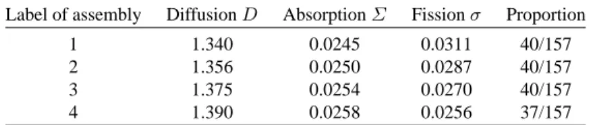
Table 1. Physical constants of the 4 types of assembly
Label of assembly DiffusionD AbsorptionΣ Fissionσ Proportion
1 1.340 0.0245 0.0311 40/157
2 1.356 0.0250 0.0287 40/157
3 1.375 0.0254 0.0270 40/157
4 1.390 0.0258 0.0256 37/157
The Lagrange multipliers are iteratively adjusted in a inner loop at each step
nof the above algorithm (this is the most delicate part of the algorithm, the case ofI ≥3phases being much more time-consuming than just two phases). Such a gradient method always converges to a (local) minimum, and its speed of convergence is partly governed by the efficiency of the line search for finding a good steptn. However, in practice we made no special efforts in optimizing the choice oftn. Neverthelees, to improve the speed of the algorithm, we have replaced the gradient method for the angleαby an application of the optimality criteria (this is a very popular principle in structural design ; see e.g. [4]). In view of Proposition 4.2 the lamination direction αn+1 is determined by the angle between ∇un and∇pn rather than by the above formula.
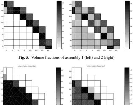
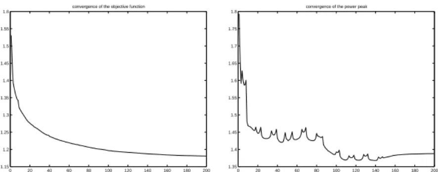
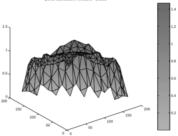
We test our method on a core with 157 squared assemblies (with side length 21.5 cm) of 4 different types with properties given by Table 1 (these data are representative of a 900 Mw pressurized water reactor). The com-putation are performed on one fourth of the geometry using the Matlab software. There are 362 P1 finite elements in the mesh and the volume fractions are constant on each assembly. We choose= 0andr = 10in the objective function (other choices work as well). We first compute the optimal solution for the relaxed formulation after 200 iterations. Figures 5 and 6 display the optimal volume fractions, and Fig. 7 the resulting power distributionσu. The convergence is smooth as shown by figure 8 and in-dependent of the initialization (we believe we reached a global minimum). The power peakmax(σu)is globally decreasing (there is no reconstruction of the fine structure of the flux).
The above relaxed or homogenized optimal solution gives a lower bound on the minimal performance of any discrete distribution of assemblies. More than that, by penalizing the intermediate values of the volume fractions, we can recover a quasi-optimal distribution of assemblies. We introduce a penalized objective function, defined by
Jpen(θ, α) =λ+(M(|su|r))1/r
M(σu) +
η
|Ω|
Ω I
i=1
θi(1−θi)dx ,
0 0.1 0.2 0.3 0.4 0.5 0.6 0.7 0.8
20 40 60 80 100 120 140 160 20 40 60 80 100 120 140 160
volume fraction of assembly 1
0.1 0.2 0.3 0.4 0.5 0.6
20 40 60 80 100 120 140 160 20 40 60 80 100 120 140 160
volume fraction of assembly 2
Fig. 5. Volume fractions of assembly 1 (left) and 2 (right)
0 0.05 0.1 0.15 0.2 0.25 0.3 0.35 0.4
20 40 60 80 100 120 140 160 20 40 60 80 100 120 140 160
volume fraction of assembly 3
0.05 0.1 0.15 0.2 0.25 0.3 0.35 0.4 0.45 0.5 0.55
20 40 60 80 100 120 140 160 20 40 60 80 100 120 140 160
volume fraction of assembly 4
Fig. 6. Volume fractions of assembly 3 (left) and 4 (right)
0 0.2 0.4 0.6 0.8 1 1.2 0 50 100 150 200 0 50 100 150 200 0 0.2 0.4 0.6 0.8 1 1.2 1.4
power distribution, k effective =1.0469
Fig. 7. Power distributionσu
0 20 40 60 80 100 120 140 160 180 200 1.15 1.2 1.25 1.3 1.35 1.4 1.45 1.5 1.55 1.6
convergence of the objective function
0 20 40 60 80 100 120 140 160 180 200 1.35 1.4 1.45 1.5 1.55 1.6 1.65 1.7 1.75 1.8
convergence of the power peak
Fig. 8. Convergence history: objective function (left) and power peak (right)
0 0.1 0.2 0.3 0.4 0.5 0.6 0.7 0.8 0.9 1
20 40 60 80 100 120 140 160 20 40 60 80 100 120 140 160
volume fraction of assembly 1
0 0.1 0.2 0.3 0.4 0.5 0.6 0.7 0.8 0.9 1
20 40 60 80 100 120 140 160 20 40 60 80 100 120 140 160
volume fraction of assembly 2
Fig. 9. Distributions of assembly 1 (left) and 2 (right)
0 0.1 0.2 0.3 0.4 0.5 0.6 0.7 0.8 0.9 1
20 40 60 80 100 120 140 160 20 40 60 80 100 120 140 160
volume fraction of assembly 3
0 0.1 0.2 0.3 0.4 0.5 0.6 0.7 0.8 0.9 1
20 40 60 80 100 120 140 160 20 40 60 80 100 120 140 160
volume fraction of assembly 4
Fig. 10. Distributions of assembly 3 (left) and 4 (right)
0.2 0.4 0.6 0.8 1 1.2 1.4
0 50
100 150
200
0 50 100 150 200
0 0.5 1 1.5
power distribution, k effective =1.0505
Fig. 11. Power distribution after penalization
Table 2. Comparison between the homogenized and penalized designs
Objective function Power peak Homogenized design 1.180 1.387
Penalized design 1.249 1.551
In Table 2 we compare the values of the objective function for the relaxed optimal design and for the penalized one (the penalization termJpen−J∗ is almost zero at the end of the penalization process).
In our opinion the interest of the homogenization method is twofold. First, the homogenized optimal design gives an absolute lower bound to any proposed discrete distribution of assemblies. Therefore, it is a good element of comparison with any other optimization method. Second, the homogenization algorithm is insensitive to the initial guess and the resulting penalized discrete distribution of assemblies is free of any implicit or explicit constraint on its pattern (in structural optimization this is called topology optimization, see e.g. [1, 3, 4]). We do not view this method as an alternative to other optimization algorithms but rather as a pre-processing step. Indeed, it gives rise to new patterns that may be different from initial guesses or intuitions, but that can be improved by local optimization using more realistic constraints or objective function.
7. Conclusion and perspectives
working in two directions. First, we generalize the present work to the more realistic model of two-groups diffusion (this is a system of two coupled dif-fusion equations). The principle of this generalization is the same but many new mathematical difficulties arise. In particular, we shall introduce a par-tial relaxation instead of the true relaxed formulation which is unfortunately untractable. Second, we have to take into account more realistic constraints in the optimization process and do more numerical comparisons with other approaches in the literature. This will be reported in a next paper [2].
References
1. Allaire G., Bonnetier E., Francfort G., Jouve F.: Shape optimization by the homoge-nization method. Numerische Mathematik 76, 27–68 (1997)
2. Allaire G., Castro C. (in preparation)
3. Allaire G., Kohn R.V.: Optimal design for minimum weight and compliance in plane stress using extremal microstructures. Eur. J. Mech. A/Solids 12(6), 839–878 (1993) 4. Bendsoe M.: Methods for optimization of structural topology, shape and material.
Berlin Heidelberg New York: Springer 1995
5. Dacorogna B.: Weak continuity and weak lower semicontinuity of nonlinear function-als. Lecture Notes in Math. 922, Berlin Heidelberg New York: Springer 1982 6. Dumas M.: Optimisation du repositionnement des assemblages combustibles d’un
r´eacteur nucl´eaire, in Numerical methods for engineering,2ndinternational congress GAMNI, E. Absi et al. eds., pp. 865-874, Paris: Dunod 1980
7. Ekeland I., Temam R.: Convex analysis and variational problems. Amsterdam: North Holland 1976
8. Gaudier F.: Mod´elisation par r´eseaux de neurones. Application `a la gestion du com-bustible dans un r´eacteur, PhD thesis, ENS Cachan (1999)
9. Ho L.-W., Rohach A.: Perturbation theory in nuclear fuel management optimization. Nucl. Sc. Eng. 82, 151–161 (1982)
10. Jikov V., Kozlov S., Oleinik O.: Homogenization of differential operators. Berlin: Springer 1995
11. Kropaczek D.J., Turinsky P.J.: In-core nuclear fuel management optimization for pres-surized water reactors utilizing simulated annealing. Nucl. Technol. 95, 9 (1991) 12. Levine S., In-core fuel management of four reactor types, in Handbook of Nuclear
Reactor Calculations, vol. II, Y. Ronen ed., CRC Press, pp. 87–201 (1986).
13. Lurie K., Cherkaev A.: Exact estimates of conductivity of composites formed by two isotropically conducting media, taken in prescribed proportion. Proc. R. Soc. Edinburgh
99A, 71–87 (1984)
14. Lysenko M.G., Wong H.I., Maldonado G.I.: Neural network and perturbation Theory hybrid Models For Eigenvalue Prediction. Nucl. Sc. Eng. 132, (1999)
15. Lysenko M.G., Wong H.I., Maldonado G.I.: Predicting Neutron Diffusion Eigenvalues with a Query-Based Adaptive Neural Architecture. IEEE Trans. Neural Network 10 (1999)
16. Maldonado G.I., Turinsky P.J.: Application of nonlinear nodal diffusion generalized perturbation theory to nuclear fuel reload optimization. Nucl. Technol. 110, 198–219 (1995)
18. Murat F., Tartar L.: Calcul des variations et Hog´en´eisation, in Les M´ethodes de l’Homog´en´eisation: Th´eorie et Applications en Physique, Eyrolles, 319-369 (1985). English translation in Topics in the mathematical modelling of composite materials. A. Cherkaev, R. Kohn, Editors, Progress in Nonlinear Differential Equations and their Applications, 31, Birkh¨auser, Boston (1997)
19. Parks G.T.: Multiobjective pressurized water reactor reload core design by nondomi-nated genetic algorithm search. Nucl. Sci. Eng. 124, 178–187 (1996)
20. Planchard J.: M´ethodes math´ematiques en neutronique, Paris: Eyrolles 1995 21. Raitum U.: The extension of extremal problems connected with a linear elliptic
equa-tion. Sov. Math. 19, 1342–1345 (1978)