Analysis and design of an edge-technique-based
Doppler wind lidar. Practical assessment of a
laboratory prototype
Ph.D. Thesis dissertation
Submitted in partial fulfilment of the requirements for the degree of
DOCTOR IN PHILOSOPHY
Submitted by
Constantino Muñoz-Porcar
Thesis advisors:
Dr. Adolfo Comerón Tejero and Dr. Alejandro Rodríguez Gómez
Analysis and design of an edge-technique-based Doppler wind lidar. Practical assessment of a laboratory prototype © 2012, Constantino Muñoz-Porcar, Adolfo Comerón-Tejero and Alejandro Rodríguez-Gómez
Remote Sensing Laboratory
Departament de Teoria del Senyal i Comunicacions
Abstract
This thesis is the initial stage in the development of a range-resolving, aerosol-return-based Doppler wind lidar. Such instruments measure the speed of the wind by detecting the Doppler frequency shift undergone by the light that is scattered by aerosols, which are taken as wind tracers, when they are illuminated by pulsed laser radiation. The detection technique considered in this work is the so-called ‘edge-technique’, where the slope of the frequency response of an optical filter is used as frequency discriminator.
The thesis is divided in two parts. In the first one, the optimal configuration of the optical filter is calculated and a complete analysis of the system performance is carried out. The second part is devoted to the design, implementation and assessment of a laboratory prototype. The objective of this development is to assess the implementation of the detection technique and to characterize and adjust the operation of some of the critical elements and subsystems that will be part of the Doppler wind lidar.
Agraïments
Vull agraïr, en primer lloc, l’ajuda i el recolzament que, al llarg d’aquests anys, en tot moment he rebut dels meus amics i directors de tesi, Adolfo Comerón i Alejandro Rodríguez. És obligatori també un reconeixement a les persones que dintre del grup de recerca i el departament han contribuït, d’una forma o altra, als resultats que es presentaran aquí: Michaël Sicard, Francesc Rocadenbosch, David Garcia, Federico Dios, Miguel Ángel López, Sergio Tomás, Diego Lange, Òscar Batet, Dhiraj Kumar, Nadzri Reba, Joaquim Giner, Carles Diaz, Josep Maria Haro, Ruben Tardío, Jordi Guillem, Josep Pastor, Albert Martón i Alfredo Cano. Tampoc puc oblidar als estudiants de Projecte Final de Carrera que han participat de forma directa en diferents etapes d’aquest treball: Alberto Muriel, Xavier Alfonso, Elena Jiménez, Maria Freixes, Joan Mercadal, Daniel Pérez, Sergi Manuel, Miguel Ángel Leo i Daniel Ballesta.
Acknowledgements
The following institutions are gratefully acknowledged for their contributions to this work: MCYT (Ministerio de Ciencia y Tecnología), MICINN (Ministerio de Ciencia e
Innovación) and ERDF (European Regional Development Fund) under the R&D projects REN2003-09753-C02-C02/CLI, TEC2006-07850/TCM and TEC2009-09106 funding the RSLAB (Remote Sensing Laboratory) - lidar.
European Commission under the ACTRIS (Aerosols, Clouds, and Trace gases Research InfraStructure Network) FP7 Grant Agreement no. 262254, the EARLINET-ASOS (European Aerosol Research Lidar Network-Advanced Sustainable Observation System) FP6 contract no. RICA-025991 and the EARLINET (A European Aerosol Research Network to Establish an Aerosol Climatology) FP5 contract no. EVR1-CT-1999-40003 funding the European Lidar Network EARLINET.
CDTI (Centro para el Desarrollo Tecnológico Industrial) under the R&D project ATLAS (Desarrollo de un instrumento de ayuda a la navegación aérea en condiciones meteorológicas desfavorables. Aplicación de Técnicas LIDAR en el sector Aeronáutico para el incremento de la Seguridad aérea) Ref. SAE-20081054 funding the RSLAB (Remote Sensing Laboratory) - lidar.
CIRIT (Comissió Interdepartamental de Recerca i Innovació Tecnològica), DURSI/DMA (Departament d'Universitats, Recerca i Societat de la Informació / Departament de Medi Ambient) under de R&D project IMMPACTE (Integració metodològica i de models per a la previsió i l'anàlisi de la contaminació i el temps i dels seus efectes) funding the RSLAB (Remote Sensing Laboratory) - lidar.
Contents
ABSTRACT ...V
AGRAÏMENTS ...VII
ACKNOWLEDGEMENTS...IX
CONTENTS ...XI
LIST OF FIGURES ... XV
LIST OF TABLES ... XIX
1 INTRODUCTION ... 1
1.1 Introduction to lidars ... 1
1.2 Background... 2
1.3 Objectives... 3
1.4 Organization of the thesis ... 4
2 DOPPLER WIND LIDARS... 7
2.1 Introduction to Doppler wind lidars... 7
2.2 History of Doppler wind lidars... 8
2.3 Types of Doppler wind lidars ... 9
2.3.1 Coherent Doppler wind lidars... 9
2.3.2 Direct-detection Doppler wind lidars ... 11
3 ELASTIC SCATTERING OF LIGHT IN THE ATMOSPHERE... 13
3.1 Frequency features of the return signal ... 13
3.1.1 Rayleigh scattering ... 14
3.1.2 Mie scattering ... 16
3.1.3 Spectral characteristics of the elastic return ... 17
3.2 The lidar signal. Temporal analysis of the elastic return... 18
3.2.1 Incident electric field and optical intensity on the receiving area... 18
3.2.2 The lidar equation... 24
4 THE EDGE TECHNIQUE... 25
4.1 The edge technique principle... 25
4.2 High resolution optical filter: The Fabry Perot interferometer ... 26
4.3 Frequency response for lidar signals ... 27
4.4.1 Precision. Uncertainty of the measurements... 29
4.4.2 Signal-to-noise ratio in optical receivers ... 30
4.4.3 Accuracy. Effect of the Rayleigh background on measurement bias ... 32
5 DESIGN AND PERFORMANCE ANALYSIS OF THE DOPPLER RECEIVER IN EDGE-TECHNIQUE-BASED LIDARS... 37
5.1 Design parameters... 38
5.2 Continuous-wave hard-target velocimeter... 38
5.2.1 Main system parameters ... 38
5.2.2 Optimization of the frequency discriminator... 39
5.2.2.1 Frequency response... 39
5.2.2.2 Sensitivity to velocity changes... 40
5.2.2.3 Signal-to-noise ratio... 42
5.2.2.4 Uncertainty-based velocity-range. Optimal cavity length... 43
5.2.3 Precision of the velocity measurements... 46
5.2.3.1 Uncertainty of the individual measurements... 46
5.2.3.2 Measurements averaging. Time resolution ... 46
5.3 Aerosol Doppler wind lidar ... 47
5.3.1 Main system parameters ... 47
5.3.2 Optimization of the frequency discriminator... 48
5.3.2.1 Frequency response... 48
5.3.2.2 Sensitivity to velocity changes... 50
5.3.2.3 Signal-to-noise ratio... 52
5.3.2.4 Uncertainty-based velocity-range. Optimal cavity length... 54
5.3.3 Precision of the velocity measurements... 56
5.3.3.1 Zero velocity location ... 56
5.3.3.2 Uncertainty along the velocity range ... 57
5.3.3.3 Measurements averaging. Range and time resolution... 57
5.3.3.4 Uncertainty dependence on the received power and the aerosol scattering ratio ... 59
5.3.4 System performance in typical measuring scenarios ... 62
5.3.4.1 Power budgets... 62
5.3.4.2 Uncertainty, range and time resolutions in typical measuring scenarios... 65
5.3.4.3 Comparison with reference examples ... 66
5.3.5 Accuracy of the measurements: Effect of Rayleigh contamination on measurement bias ... 68
5.4 Conclusions of this chapter... 70
6 CONTINUOUS-WAVE SOLID-TARGET PROTOTYPE ... 71
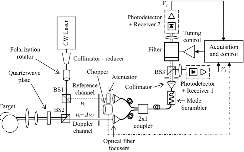
6.1 General description of the prototype ... 71
6.2 Detailed description of the prototype ... 73
6.2.1 Laser source... 73
6.2.2 Beam reducer - collimator ... 73
6.2.3 Polarization rotator ... 74
6.2.4 Beam-sampler... 74
6.2.5 Target... 74
6.2.6 Transmitting - receiving optical assembly... 75
6.2.7 Optical chopper ... 77
6.2.8 Optical fiber focusers... 78
6.2.9 Optical fibers ... 78
6.2.10 Optical fiber 2×1 coupler... 79
6.2.11 Mode scrambler ... 79
6.2.12 Collimator... 80
6.2.16 Other parts of the experimental setup ... 84
6.3 Retrieval of the frequency response from the detected voltages ... 86
6.4 Retrieval of the Doppler frequency from the frequency response ... 87
6.5 Tuning control subsystem... 88
6.6 Routines and procedures ... 89
6.6.1 Offset-voltages calibration stage ... 89
6.6.2 Frequency response calibration stage ... 90
6.6.3 Measurement and tuning control stage ... 91
7 MEASUREMENTS... 95
7.1 Interferometer performance... 95
7.1.1 Example of acquisition of the frequency response ... 95
7.1.2 Errors due to variations of the frequency response... 96
7.1.3 Stability of the frequency response... 97
7.1.4 Degradation of the frequency response ... 101
7.1.5 Dependence of the frequency response with the point-of-impact on the target... 102
7.1.6 Differences between the frequency response in the reference and the Doppler channel ... 102
7.2 BS3 splitting-ratio. Normalization constant... 103
7.3 Tuning control system... 104
7.3.1 Estimation of the frequency drifts compensated by the system... 104
7.3.2 Effect of ‘sensitivity’ and ‘interval’ parameters ... 106
7.4 Velocity measurements ... 108
7.4.1 Description of the tests ... 108
7.4.2 Power conditions ... 109
7.4.3 Expected uncertainty in the velocity determination... 110
7.4.4 Bias error in the velocity determination ... 113
7.4.5 Velocity measurements... 113
7.4.5.1 Results... 114
7.4.5.2 Analysis of the bias error ... 119
7.4.5.3 Analysis of the uncertainty... 119
8 CONCLUSIONS AND FURTHER WORK ... 121
8.1 Conclusions ... 121
8.2 Further work ... 123
8.2.1 Implementation of an edge-technique-based Doppler wind lidar... 123
8.2.2 Implementation of a double-edge-technique-based Doppler wind lidar... 124
8.2.3 Rayleigh-based measurements... 124
LIST OF SYMBOLS, ACRONYMS AND ABBREVIATIONS... 127
REFERENCES... 135
List of figures
Fig. 1. Scheme of a coherent Doppler lidar detector....10
Fig. 2.Principle of operation of direct-detection techniques based on frequency to intensity conversion. Edge technique (left) and double-edge technique (right). 0 is the emitted frequency, fD is the Doppler frequency shift between received and emitted signals, F(), F1() and F2() are the frequency responses of the optical filters used to perform the frequency to intensity conversion (in this case Fabry-Perot interferometers) and F, F1 and F2 are the changes in the filters transmission, due to frequency changes, to be detected....11
Fig. 3.Principle of operation of a lidar based on the fringe-imaging technique, in this case using a Fabry-Perot interferometer as frequency discriminator....12
Fig. 4. Effect of collisions of air molecules on the spectrum of the backscattered radiation. Mean free path between collisions after the US Standard Atmosphere Model, 1976 (left); Rayleigh-Brillouin normalized backscatter spectra at 355 nm around the central backscatter frequency at sea level (dash-dotted curve) and 5000 m (dashed curve) calculated using the Pan s7 model [42]; the continuous curve represents the ideal Rayleigh scattering at 5000 m (right) [43]....15
Fig. 5. Aerosol backscatter coefficient. Dependence with wavelength [46]....17
Fig. 6. Spectral features of the emitted pulse and the elastic return. L,M and R are respectively the spectral width of the emitted pulse, the Mie component and the Rayleigh component of the elastic return and fD is the Doppler frequency shift between the received components and the emitted pulse....18
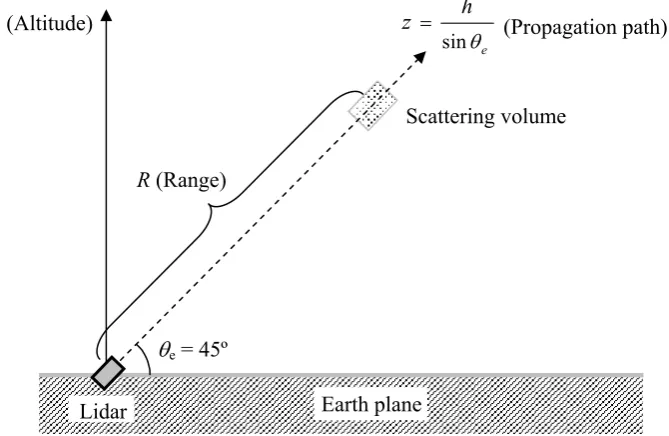
Fig. 7. Lidar in monostatic configuration and the geometrical arrangement....19
Fig. 8. Field temporal envelope...20
Fig. 9. Atmospheric layer of thickness z at distance R....21
Fig. 10. Calculation of the coherence area over the telescope plane....23
Fig. 11. Principle (left) and a basic layout (right) of an Edge Technique system....26
Fig. 12. Graphic representations of the transmission function of a Fabry-Perot interferometer....27
Fig. 13. Photodetection process in an optical receiver (after ref. [56]) ...31
Fig. 14. Edge-technique-based Doppler wind lidar with detection of the Rayleigh component. Filter 1 is used for the edge-technique implementation while Filter 2 helps to determine the Rayleigh component in the detected signals....34
Fig. 15. Mie and Rayleigh responses of filter 2, along with the spectrums of the emitted pulse and the return at the extremes of the measurable velocity range (HMFW = 500 MHz, velocity range is ±25 m/s, T = 300ºK, p = 10 ns and 0 = 1064 nm)....35
Fig. 16. CW frequency response for configurable values of the cavity length when F = 45....40
Fig. 17. Bandwidth of the CW frequency response as a function of the cavity length for different values of the finesse....40
Fig. 18. Sensitivity to velocity changes along the slope for different values of the cavity length when F = 45....41
Fig. 20. Signal-to-noise ratio of the frequency response measurement along the slope, when
Pin = 100 nW and no averaging is performed...43
Fig. 21. Calculated uncertainty of the measurements along the slope of the filter for different configurable values of the cavity spacing (d), when Pin = 100 nW and no averaging is performed....44
Fig. 22. Definition of the uncertainty-based velocity-range using the calculation of the measurement uncertainty as a function of the measured radial velocity....44
Fig. 23. Frequency response of a Fabry- Perot interferometer to pulsed light (F = 35,d = 3.6 cmand p = 10 ns)....49
Fig. 24. Frequency response for configurable values of the cavity length for F = 35 and p = 10 ns....49
Fig. 25. Maximum transmission and bandwidth of the frequency response as a function of the cavity length for F = 35 and p = 10 ns....50
Fig. 26. Sensitivity to velocity changes (F = 35, d = 3.6 cm, p = 10 ns and = 1064 nm)...51
Fig. 27. System Sensitivity to velocity changes along the filter slope for different configurable cavity lengths for F = 35, p = 10 ns and = 1064 nm....51
Fig. 28. Maximum system sensitivity and sensitivity-based velocity-range as a function of the cavity length for F = 35, p = 10 ns and = 1064 nm....52
Fig. 29. Signal-to-noise ratio for PM = 10 nW, ASR = 2 and AF = 1000, for different values of the cavity length....54
Fig. 30. Calculated uncertainty PM = 10 nW, ASR = 2 and AF = 1000 for different values of the cavity length....54
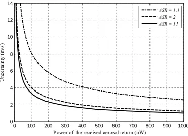
Fig. 31. Mean uncertainty (along the whole velocity measurable range) as a function of the Mie return power for different values of the ASR (d = 2.4 cm, F = 35, p = 10 ns and = 1064 nm)....59
Fig. 32. Signal-to-noise ratio dependence on the aerosol received power for different values of the aerosol scattering ratio....60
Fig. 33. Uncertainty dependence on the aerosol scattering ratio for different values of the incident Mie return power....61
Fig. 34. Signal-to-noise ratio (mean value in the measurable velocity range) dependence on the aerosol scattering ratio for different values of the incident Mie return power....61
Fig. 35. Aerosol scattering ratio profiles used for power calculations...63
Fig. 36. Orientation of the observation for horizontal wind measurements....64
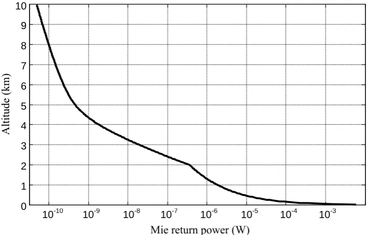
Fig. 37. Mie return power in an atmosphere with the aerosol load described by profile I....65
Fig. 38. Absolute error in the determination of the frequency response along the filter slope as a function of the detected velocity for different atmospheric conditions...69
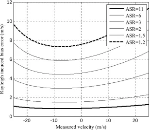
Fig. 39. Rayleigh-induced bias error in frequency determination within the velocity dynamic range (F = 35, d = 2.4 cm, p = 10 ns, = 1064 nm and f0 = 83.1 MHz)....69
Fig. 40. General scheme of the continuous-wave solid-target prototype...72
Fig. 41. Beam reducer - collimator...73
Fig. 44. Voltage-controlled rotating disc...75
Fig. 45. Polarization processing in the transmitting – receiving optical assembly...76
Fig. 46. Focusing system in the transmitting – receiving assembly....76
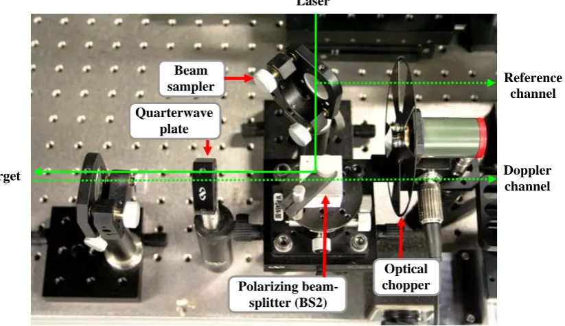
Fig. 47. Beam sampler, transmitter-receiver assembly and optical chopper....77
Fig. 48. Elements in the focusing system...78
Fig. 49. Optical fiber focusers. Their function is to couple the light from the reference (A) and Doppler (B) channels to their respective optical fibers....79
Fig. 50. 2x1 coupler and mode scrambler....80
Fig. 51. Collimating system and maximum divergence...80
Fig. 52. Collimator...81
Fig. 53. Interferometer controller....82
Fig. 54. Scheme of the photoreceivers....82
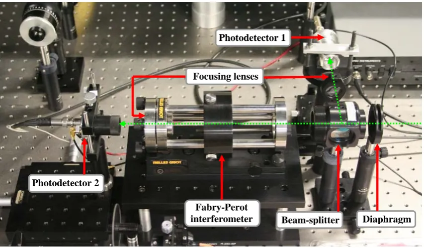
Fig. 55. The Doppler detection section of the prototype....83
Fig. 56. Electronic devices not appearing in the previous sections: Chopper controller (1), high-voltage power supplies (2) (one for each photodetector), low-voltage power supply (3), transimpedance amplifiers (4) (one for each photodetector) and BNC connector block for the acquisition card (5)....84
Fig. 57. Optical section of the laboratory set-up: Laser (1), reducer-collimator (2), polarization rotator (3), beam-sampler (4), polarizing beam-splitter (5), quarterwave plate (6), lens 1 of the focusing system (7), optical chopper (8), attenuator (9), optical fiber focusers (10), 2x1 optical fiber coupler (11), mode scrambler (12), optical fiber end (13), collimating lens (14), diaphragm (15), beam-splitter (16), Fabry-Perot interferometer (17) and photodetectors (18)....85
Fig. 58. Another general view of the laboratory set-up. The numeration is the same than the one defined in the title of Fig. 57....85
Fig. 59. Doppler shift measurement from the normalized frequency response...87
Fig. 60. Scheme of the tuning control subsystem...88
Fig. 61. Complete sequence of routines in a session of velocity measurements....89
Fig. 62. Time-to-frequency sampling interval translation....90
Fig. 63. Schematicstructure of the frequency response calibration routine....91
Fig. 64. Frequency response calibration routine: Control panel....91
Fig. 65. Acquired signals during the measuring stage....92
Fig. 66. Correction of the laser location...93
Fig. 67. Schematic structure of the measurement and tuning control routine. ...93
Fig. 68. Frequency response acquired during calibration. d = 4 cm; F = 47.62; HWHM = 39.37 MHz...96
Fig. 69. Error in velocity determination due to an error in the frequency response for different measured linear speeds....97
Fig. 70. Finesse evolution in successive scans during 20 minutes (Test I)....98
Fig. 71. Finesse evolution in successive scans during 20 minutes (Test II)....98
Fig. 73. Finesse evolution in successive scans during 20 minutes (Test IV)....99 Fig. 74. Velocity error due to variations of the normalization factor in the Doppler channel. k
= 0.8, F = 47.62, cavity length d = 4 cm, operation wavelength 0 = 1064 nm....104 Fig. 75. 2 minutes monitoring of the voltage that controls the cavity length with ‘sensitivity’
equal to 1 % and ‘interval’ 50 ms (see section 6.6.3)....105 Fig. 76. 2 minutes monitoring of the voltage that controls the cavity length with ‘sensitivity’
equal to 4 % and ‘interval’100 ms (see section 6.6.3)....105 Fig. 77. Increase in mean uncertainty due to non-compensated frequency drifts as a function
of the parameter ‘interval’....107 Fig. 78. Increase in mean uncertainty due to non-compensated frequency drifts as a function
of the parameter ‘interval’....107 Fig. 79. Location of the emitted frequency and the frequency dynamic range of the
measurements. Optimal location (left) and maximum allowed displacement (right)....108 Fig. 80. Measurement points listed in Table 39....109 Fig. 81. Expected velocity uncertainty due to the photoreceiver noise as a function of the
measured velocity, when no averaging is performed....112 Fig. 82. Expected velocity uncertainty according to the measured fluctuations of the frequency
response and point-of-impact dependence of the frequency response and the splitting
ratio in the Doppler channel....112 Fig. 83. Measured velocities and uncertainty vs. ’true’ radial velocity with no averaging (Test
I)...115 Fig. 84. Measured velocities and uncertainty vs. ‘true’ radial velocity with no averaging (Test
II)...116 Fig. 85. Measured velocities and uncertainty vs. ‘true’ radial velocity with no averaging (Test
III)...117 Fig. 86. Measured velocities and uncertainty vs. “true” radial velocity with no averaging
(Test IV)...118 Fig. 87. Comparison between the uncertainty obtained in each test and the expected
List of Tables
Table 1. Parameters of the laser, the optical receiver and the optical filter in the
continuous-wave prototype....39
Table 2. Uncertainty-based velocity-range for configurable cavity lengths....45
Table 3. Average uncertainty within the measurable velocity range for useful values of the cavity length....46
Table 4. Uncertainty parameters (d = 4 cm, F = 45)....46
Table 5. Mean uncertainty when sample averaging is applied (d = 4 cm, F = 45)...47
Table 6. Required averaging factor for different values of uncertainty and incident power (d = 4 cm, F = 45)...47
Table 7. Parameters of the laser, the telescope, the optical receivers and the optical filter in the aerosol system....48
Table 8. Uncertainty-based velocity-range for configurable cavity lengths....55
Table 9. Mean uncertainty along the measurable frequency range for usable values of the cavity length....56
Table 10. Position of the point with minimum uncertainty for d = 2.4 cm, F = 35, p = 10 ns and = 1064 nm....57
Table 11. Uncertainty parameters for d = 2.4 cm, F = 35, p = 10 ns, = 1064 nm and f0 = 87.3 MHz....57
Table 12. Required averaging factor for achieving a given mean uncertainty within the measurable frequency range (d = 2.4 cm)....58
Table 13. Range – time resolution combinations to achieve 0.2, 1 and 2 m/s uncertainty for each value of the Mie return power....58
Table 14. Typical lidar ratios for different aerosol types at 532 nm wavelength determined with a Raman lidar [58]...63
Table 15. Power calculations at different measuring scenarios...64
Table 16. Mean uncertainty for different measuring situation with different range – time averaging combinations...65
Table 17. Averaging factor and example of resolution combination to obtain fixed values of uncertainty in different measuring situations....66
Table 18. Standard requirements of wind measurements for space-borne global wind measurements and performance parameters of a coherent lidar used for windshear detection....67
Table 19. Mean Rayleigh-induced bias error within the velocity dynamic range...68
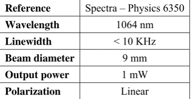
Table 20. Main parameters of the Continuous-wave laser...73
Table 21. Parameters of the beam reducer – collimator lenses...73
Table 22. Parameters of the transmitter-receiver assembly lenses...77
Table 23. Parameters of the optical fiber focuser...78
Table 24. Parameters of the optical fiber...78
Table 26. Parameters of the collimating lens...80
Table 27. Main parameters of the Fabry-Perot interferometer...82
Table 28. Parameters of the APD...83
Table 29. Parameters of the amplifier...83
Table 30. Standard deviation of the measured finesse and the zero-velocity corresponding velocity error when no averaging is performed....100
Table 31. Finesse and velocity standard deviation when 20 and 100 scans are averaged....101
Table 32. Two minutes partial mean finesse....101
Table 33. Statistics of the point-of-impact dependence of the averaged measured finesse for the Doppler channel....102
Table 34. Bias error in the velocity determination due to differences between the mean frequency response in the Reference and the Doppler channel....103
Table 35. Statistics of the point-of-impact dependence of the normalization factor for the Doppler channel...104
Table 36. Increase in mean uncertainty due to non-compensated frequency drifts as a function of the parameter ‘interval’....106
Table 37. Increase in mean uncertainty due to non-compensated frequency drifts as a function of the parameter ‘sensitivity’....106
Table 38. Velocity tests configuration parameters....109
Table 39. Optical power measured (non-shaded) and estimated (shaded) at different points of the prototype set-up....110
Table 40. Partial and overall expected uncertainty...113
Table 41. Main settings and parameters of the velocity tests...114
Table 42. Results for test I...115
Table 43. Results for test II...116
Table 44. Results for test III...117
1
Introduction
1.1
Introduction to lidars
Lidars, also known as laser-radars, are optical remote sensing systems, that is, they explore distant objects using light as vehicle for the information. Remote sensing using light is not of course a modern invention. Seeing is something that many animals do since they are born to acquire information about the surrounding world. Since the appearance of intelligence, however, humans have used technology to enhance this natural capability. As probably the first example, as soon as men were able to light a fire, they surely used it to illuminate objects in the dark. This was, actually, an active technique for improving their visual capability: they emitted the light that, after being scattered by objects, was detected by their eyes and permitted, in naturally adverse conditions for vision such as night time or inside dark caves, obtaining information about them. In essence, what lidars do is not much different; the source of light in the case of lidars, however, is a laser (instead of a torch), the detector is formed by a telescope and an optoelectronic receiver (instead of the human visual system) and, according to their respective characteristics, the type of information that lidars help to become ‘visible’ is usually as well different.
development of optoelectronics provided the technologies required for efficiently adapting these techniques to the optical frequencies. In fact, both denominations: laser-radar and lidar which is an acronym of Light Detection And Ranging (as an optical version of the one first used for radars: Radio Detection And Ranging), reveal eloquently this inheritance.
The range of wavelengths used by laser-radars, occupying in most of applications near-ultraviolet, visible and near-infrared frequency bands, determines some of their unique features as remote sensing instruments. At these frequencies, the electromagnetic radiation interacts in some cases strongly with the atmospheric constituents. Lidars, taking advantage of this interaction, can be used for deriving range-resolved information of the atmosphere state. Atmospheric science has indeed stood out as one of the main fields of application of lidar technologies. A manifold of atmospheric variables such as temperature, pressure, speed of the wind or content of aerosol particles, water vapour and trace gases, whose knowledge is important for understanding and modelling the complex processes that govern the atmospheric dynamics, have been successfully profiled using lidar instruments. Their main advantages with respect to the traditional in situ techniques, applied from sounding rockets or balloons for atmospheric profiling, are higher spatial and temporal resolution and the possibility of continuous monitoring. Radars are also used in atmospheric research and their capabilities are a good complement of lidar ones. While lidars, which need clean-air conditions to operate, are capable to measure gases and aerosols, radars rely on the scattering from atmospheric hydrometeors and are therefore better suited for rainfall monitoring, thunderstorm tracking or cloud profiling.
1.2
Background
Lidar activities started in the Universitat Politècnica de Catalunya (UPC) in 1993. Since then, three lidar systems, dedicated mainly to measure and monitor atmospheric aerosol particles have been developed by the Lidar Group of the UPC and have been exploited in the frame of different national and international projects. This thesis is related to the aim of the
UPC lidar group to extend its activity scope developing a Doppler wind lidar.
comparing the transmittance of optical filters. There exist, however, two variations of this method: the single-edge-technique or simply edge-technique, which uses only one filter, and the double-edge-technique, a more sophisticated and sensitive version using two filters. The edge-technique is the version that, for simplicity issues, will be implemented as a first step. Edge-technique wind lidars can be in turn designed to rely either on aerosol (Mie) [5] or on molecular (Rayleigh) backscatter [2]. The proposed Doppler wind lidar will be in principle a ground-based station that will be housed in the UPC facilities in Barcelona, an urban area at sea level, where the mixing boundary layer is usually heavily aerosol-loaded. Aerosol-based systems are under these conditions better suited for wind measurements than the ones relying on molecular return. They are as well technologically less demanding as they are inherently more sensitive. In conclusion, the Doppler wind lidar that the UPC group has finally decided to develop will use the edge-technique and will operate relying on aerosol scattering. The work presented in this Ph. D. thesis has been therefore carried out in the frame of the general objective of developing a system with such characteristics.
1.3
Objectives
The first part of this thesis has been devoted to carry out the performance analysis and the optimization of the detection unit of an edge-technique-based Doppler wind lidar. The performance of the detection system is first analyzed in terms of precision (uncertainty) in the velocity measurements as a function of the configuration of the frequency discriminator, the incident optical power and the proportion of interfering Rayleigh component in the return signal. The results of this analysis permit to optimize the configuration of the proposed optical frequency discriminator (a Fabry-Perot interferometer). Power budgets for the planned UPC system in different measuring scenarios are then calculated. Precision parameters (uncertainty and range-time resolution) are calculated and are compared with standard reference examples. The effect of Rayleigh contamination both on the precision and on the accuracy (bias) of the measurements has been also studied in detail. Partial milestones of this part have been:
Derivation of the expressions necessary for analyzing the precision and the accuracy of the measurements for an edge-technique-based Doppler lidar.
Analysis of the precision (uncertainty) of the measuring system as a function of the configuration parameters of the frequency discriminator, the incident power and the Rayleigh contamination.
Definition and application of an objective criterion for optimizing the configuration of the frequency discriminator of the Doppler receiver.
Calculation of the power budgets of the UPC system under different measuring scenarios using the optimal configuration of the frequency discriminator.
Analysis of the precision of the UPC system under different measuring scenarios. Comparison with reference examples.
Analysis of the harmful effects of the molecular scattering on the accuracy (bias) of the aerosol-based wind measurements and demonstration of a possible solution.
radiation in order to achieve both range resolution and high-peak-power transmitted light pulses, which are indispensable for atmospheric sounding. However, dealing with pulsed atmospheric lidar signals is demanding: they are neither constant nor predictable and their duration is very short. Furthermore, it is difficult to validate the measurements since the true measured velocity is a priori unknown and is not easily measurable by independent means. For assessing the detection technique in controlled and convenient conditions, avoiding these difficulties, the laboratory set-up uses continuous-wave radiation and measures the velocity of hard targets. The performance analysis and the optimization of the Doppler receiver in such a version of the edge-technique-based Doppler lidar have been also carried out and are included in the first part of this work along with the study of the pulsed atmospheric case. Milestones of this part are:
Design and implementation of the continuous-wave, hard-target laboratory prototype. Design and implementation of the calibration, control and measurement procedures and
routines.
Design and implementation of a tuning control loop for stabilizing the frequency discriminator with respect to the transmitted beam.
Assessment and characterization of the Fabry-Perot interferometer as frequency discriminator.
Assessment and characterization of the tuning control loop.
Analysis of practical velocity measurements in terms of uncertainty (statistical noise) and bias error.
Comparison with the expected performance.
1.4
Organization of the thesis
Chapters 2 and 3 treat fundamental introductory subjects. Chapter 2 is dedicated to explain the basis of Doppler wind lidars. First, their main characteristics and applications and a brief history are described. Afterwards, the different techniques that can be used for detecting the Doppler frequency shift in the return signal are classified and their respective principles, applications and main characteristics are revised.
The main characteristics of the lidar signal (the one collected by the telescope after being scattered by the atmosphere) are reviewed in Chapter 3. The spectral width and the wavelength dependence are important for determining some system parameters. The lidar equation, derived after a complete temporal analysis, is indispensable for calculating power budgets and quality parameters of the velocity measurements.
In Chapter 4, the edge technique is presented and analyzed. Its principle is described, some quality parameters concerning the precision of the velocity measurements, such as the sensitivity to velocity changes, the signal-to-noise ratio and the uncertainty are defined and the expressions for calculating them are derived. The effect of Rayleigh component on the accuracy of the aerosol-based measurements is analyzed in detail too.
has been built to assess the measuring technique and secondly, a pulsed atmospheric wind lidar. In both cases, results are obtained as a function of the incident power, independently of the power budget of the system. Power budgets, quality parameters trade-offs and calculations about the effect of molecular contamination of the aerosol signals are included as well in this chapter.
In Chapter 6, a complete description of the laboratory continuous-wave prototype is presented. The expressions used to retrieve the velocity of the target from the detected voltages are derived. The measuring procedures and the schemes of the different routines that have been programmed and used for the velocity measurements are also described in detail. Experimental results obtained with the laboratory prototype are reported in Chapter 7. Several practical measurements, whose objective is the validation of the implementation of the edge-technique as method to detect the velocity, have been made and are reported and analyzed in this chapter. Firstly, however, the performance of the frequency discriminator and the tuning control loop have been tested and carefully characterized.
2
Doppler wind lidars
2.1
Introduction to Doppler wind lidars
Remote spatially-resolved wind-speed measurements are required in many fields. Ground-based [6] and space-borne [7], [8] wind measurements can provide valuable insight in atmospheric dynamics with applications in meteorology and climate science. Global atmospheric wind profiles, from ground to 120 km, have special importance for the improvement of atmospheric analysis, being useful for climate research, numerical weather forecast, modelling of stratospheric transport and, in geophysical research, for improving gravity wave parameterization in models [7], [8], [9]. In the field of air-traffic safety, typical applications include detection and tracking of air turbulence, wind shear, gust fronts or aircraft wake vortices and true air speed (TAS) indicators [1], [7], [10], [11]. In the area of electrical power generation, the installation of wind farms has experienced an important growth in the last years. Large wind turbines are installed often in complex terrains, offshore, in forests, etc. Thus, flexible and accurate wind measurements become indispensable for site testing and operation optimization [12], [13]. In all these areas and others, the research community has been looking for wind velocity measurements with higher resolution, both in space and time, than that provided by the traditional techniques such as rawinsondes, jimspheres, or anemometers in ground stations, buoys, ships and aircrafts.
advantages of lidars are smaller dimensions –which makes them better suited for mobile platforms– and narrower transmitted beams –which provides higher spatial resolution in wind profiling. On the other hand, their inability to operate under adverse weather conditions stands out as their main drawback. Regarding the basic measurement used to obtain the wind speed, wind lidar techniques can be classified into two basic categories: Doppler techniques and aerosol-inhomogeneity-tracking (direct motion detection) techniques. Doppler techniques measure the motion of the major constituent molecules of the atmosphere, N2 and O2, hence
of the wind, or of particles suspended in the atmosphere (aerosols), which are taken as wind tracers, by determining the Doppler shift undergone by the backscattered radiation. According to the Doppler effect, the frequency shift of the backscattered light ( fD) is directly related to the wind speed in the line-of-sight direction ( ): vr
0 2
D r
f v
(1)
Where 0 is the emitted wavelength and the speed is counted positive when the wind is moving away from the instrument. Aerosol-inhomogeneity-tracking techniques rely on the existence of aerosol spatial inhomogeneities –a common situation in the mixing layer– whose motion is tracked by processing the direct-detected backscatter lidar profiles along one or several line of sights.
Doppler techniques can be in turn broadly classified into two groups: coherent and direct-detection techniques. Coherent systems measure the Doppler shift using heterodyne techniques that extrapolate to the optical domain radio-frequency radar techniques. Their operation is based on mixing the return signal with a frequency-stable local oscillator (a laser beam) on a wideband optical detector; the resulting intermediate-frequency signal is processed for estimating its spectral peak. This technique offers enhanced photoreceiver sensitivity and high precision, but technological constraints limit its operation to the infrared region, where molecular return is weak and, as a result, its applicability is restricted to regions with high aerosol content, basically within the planetary boundary layer. Direct-detection-based Doppler wind lidars use optical frequency discriminators to spectrally resolve, prior to detection, the return optical signal. In this case, no technological restrictions prevent their operation in the ultraviolet region, where molecular return is strong. Wind measurements in aerosol-free conditions are thus possible, making currently this technique the preferred one for wind profiling in the mid and upper troposphere and in the stratosphere.
2.2
History of Doppler wind lidars
The origin of Doppler wind lidars is traced back to the success of laser Doppler velocimetry using coherent techniques for measuring flows in wind tunnels and high speed jets in mid sixties [14]-[16]. In 1967, Jelalian and Huffaker [17] applied this technique for the first short-range atmospheric wind velocity measurements using a continuous-wave CO2 laser operating
at 10.6 m. Later development of successive generations of coherent lidars has been related to advances on laser technology. The appearance of CO2 pulsed lasers based on the master
oscillator / power amplifier architecture (MOPA) in the early seventies, made possible longer range observations and better range resolution [18], [19] and the transverse excited atmospheric technology (TEA) permitted, in the early eighties, CO2 lasers increasing the
safety and stricter optical requirements for coherent detection associated to shorter wavelengths, provided smaller size, long life operation and higher backscatter coefficients and velocity resolution. Eye safety and higher atmospheric transmission encouraged in the first nineties the development of coherent lidars using solid-state transmitters operating at wavelengths close to 2 m (e.g. Tm,Ho:YAG at 2.09 m [21] or Tm:YAG at 2.01 m [22]). Successive improvements have since been achieved in measurement capabilities of the 2 m solid-state systems, reducing their size and power requirements and increasing their reliability. Finally, a great deal of effort has recently been addressed to the development of systems based on fiber lasers at 1550 nm, with MOPA architecture, which offer evident advantages of availability and reliability [23].
Concerning direct-detection techniques the first measurements of atmospheric wind velocity were reported by Benedetti-Michelangeli and co-workers in 1972 [24]. However, the lack of a suitable reliable high-power-pulse laser limited these measurements to distances of only several hundreds of meters. The availability of single-mode high-power solid-state transmitters in the mid eighties was the starting point for developing systems that, operating in the visible and ultraviolet regions, and using direct-detection techniques, were able to measure wind velocities relying on molecular return. Different techniques were proposed, analyzed and implemented since the late eighties, and several systems have been operated from ground-based or mobile stations for wind profiling of the atmosphere [3], [25], [26], [27], [28]. Demonstrated clean-air measuring capabilities made direct-detection techniques candidates to be flown in space-borne platforms for measuring global scale wind fields. In 2000, the European Space Agency started the technical development of the Atmospheric Dynamics Mission (ADM-Aeolus), whose launch is scheduled for 2013 and includes a Doppler wind lidar instrument based on direct-detection techniques for space-borne global observations [29]. The objective of a joint NASA, NOAA and US Department of Defense mission is to field by 2022 the Hybrid Doppler Wind Lidar (HDWL) on a research satellite. The system will use both coherent detection for accurate observations when sufficient aerosols or clouds exist and molecular direct-detection techniques above 2 km [30].
2.3
Types of Doppler wind lidars
2.3.1 Coherent Doppler wind lidars
Fig. 1. Scheme of a coherent Doppler lidar detector.
Enhanced sensitivity is one of the features of coherent optical detection. The combination on the optical detector of a weak optical signal (the received one) with the strong local oscillator laser results in a beat signal whose power is proportional to the power of both. If the power of the local oscillator is big enough, the total noise is also proportional to it and, as a consequence, the signal-to-noise ratio only depends on the signal power. In this situation, the signal-to-noise ratio is limited by the quantum noise in the signal detection and is the maximum possible (quantum-limit) [31], [32], [33].
Also, optical background noise is typically not a problem in coherent lidars for two reasons: it is not phase coherent and therefore does not mix efficiently with the local oscillator on the photodetector and most of the background photons that do produce a heterodyne beat fall outside the electronic pass band of the receiver [32].
On the other hand, the main drawback of coherent detection is its difficulty to deal with zones with low aerosol content. In these regions, which include large zones of the southern hemisphere, the central regions of the oceans and practically the whole atmosphere above the boundary layer, molecular return must be used. The dependence with the operating wavelength of the corresponding Rayleigh backscatter coefficient is proportional to -4 and as
a result, short, ultraviolet wavelengths are the optimal for wind molecular measurements. Optical heterodyne detection suffers from important technological restrictions at short wavelengths. First, the requirements on the alignment and on the optical surface quality of the telescope are stricter than at longer wavelengths. Also, the wavefront degradation effects due to atmospheric refractive turbulence are more harmful, affecting to the spatial coherence of the backscattered light and, as a consequence, to the heterodyne detection efficiency [18], [34]. Moreover the large spectral width of the beat signal arising from the molecular scattering (see section 3.1.1) would require large bandwidths in the electrical part of the photoreceiver and put heavy constraints in the acquisition system and data processing. These technological issues limit the operation of coherent Doppler Wind Lidars to the infrared region, roughly between 1 and 10 m, where aerosol return is dominant.
The coherent detection is therefore an extremely sensitive technique that has been widely used in wind Doppler lidar and is the preferred one for measurements in most of the continental regions in the lower troposphere, where the concentration of aerosols is high.
Tel
escope
Laser
tran
smitter
fD LO - (fD)
Lowpass Filter
LO
(CW)
Photo-detector Frequency
shifter
Spectral Estimation
Reference FS
2.3.2 Direct-detection Doppler wind lidars
Unlike coherent systems, direct-detection Doppler wind lidars do not use optical heterodyne mixing, previous to frequency analysis, for measuring the Doppler shift in the return signal. Instead, the collected light is spectrally analyzed prior to detection by using optical frequency discriminators [2], [4], [24]. Two basic types of frequency discriminator are used in direct-detection systems. The first group is formed by high resolution optical filters, like Fabry-Perot interferometers or filters based on molecular absorption lines, in which their frequency response is used to convert frequency shifts into changes of the detected optical intensity. This technique is usually called ‘Edge Technique’ or ‘Double-Edge Technique’ if the system uses two filters to discriminate frequencies. Fig. 2 shows this principle for both variants of the technique. Fre que nc y re sp ons es F1 ( ), F2 ( )
Frequency () fD
Fre que nc y re sp ons e F ( )
F (Received)
fD
0
(Emitted)
Fig. 2. Principle of operation of direct-detection techniques based on frequency to intensity conversion. Edge technique (left) and double-edge technique (right). 0 is the emitted frequency, fD is the Doppler frequency shift between received and emitted signals, F(), F1() and F2() are the frequency responses of the optical filters used to perform the frequency to intensity conversion (in this case Fabry-Perot interferometers) and F, F1 and F2 are the changes in the filters transmission, due to frequency changes, to be detected.
A second group of direct-detection receivers use fringe pattern imaging instruments as frequency discriminators. Systems using this technique resolve the backscattered Doppler shift by projecting the interference pattern from an optical interferometer onto a multichannel detector. In the case of using a Fabry-Perot interferometer, only angles fulfilling the resonance condition into the cavity (2dcos = m, where is the incidence angle onto the etalon, d is the cavity length and m is an integer number [35]) will be completely transmitted and, as a result, the output of the interferometer, properly imaged, will be a collection of concentric rings. The transmitted angles, and consequently the position of the rings, depend on the incident wavelength. The Doppler shift is obtained measuring the angular displacement of the fringe locations (Fig. 3).
Direct-detection Doppler wind lidars are suited to operate in the ultraviolet region and therefore can measure in aerosol-free conditions. This stands out as their main advantage with respect to lidars based in coherent detection and makes them a good choice for measuring global-scale wind fields from space-borne stations and for stratospheric wind profiling. However, although current interest on non-coherent systems is mainly due to their capability for measuring winds in aerosol-free conditions, and particularly to their suitability for space-borne applications, all direct-detection techniques can be also applied for aerosol (Mie) return. Although their performance is, in aerosol-loaded regions, worse than the one of coherent systems, some advantages like their flexibility to be easily adapted to molecular
Frequency ()
Emitted (0)
Received filter 1
F2
F1
F2
F1
Received filter 2
→ fD
measurements and the possibility of using shorter pulses make them an interesting option in some cases. In such conditions, however, some of the main design parameters of the receiver and the performance of the measuring system are different from those of molecular-return-based systems.
d
Fabry-Perot etalon Imaging optics
n
Detector plane
r
n
Extended source
Fig. 3. Principle of operation of a lidar based on the fringe-imaging technique, in this case using a Fabry-Perot interferometer as frequency discriminator.
3
Elastic scattering of light in the atmosphere
Lidar systems retrieve information of the state of the atmosphere by analyzing the electromagnetic energy that is scattered when it is illuminated with a laser beam. Different contributions to the overall scattered energy can be identified and classified depending on the characteristics of the physical phenomenon responsible of it. A first classification is established between elastic and non-elastic scattering processes. By elastic scattering it is understood that one in which the energy of the incident photons, and therefore their frequency, is conserved and only their direction changes. Elastic scattering can be, in turn, classified in Mie and Rayleigh scattering. Mie scattering refers to elastic scattering in aerosol particles whose size is comparable or larger than the wavelength of the incident radiation, while Rayleigh scattering is produced in particles whose size is much smaller than the incident wavelength, including the molecules of the constituents of the atmosphere. Doppler wind lidars measure the wind speed by detecting the frequency shift, due to Doppler effect, that is undergone by the radiation that is elastically scattered either by the air molecules or by the suspended particles. An accurate analysis and the design of any Doppler wind lidar require taking in account the main characteristics of the return signal due to elastic scattering. In this chapter, these characteristics will be discussed and several analytical expressions will be derived in terms of transmitter, receiver and atmospheric parameters.
3.1
Frequency features of the return signal
a distance proportional to the time elapsed since the emission and with a thickness that depends on the pulse duration [37]). If all the scatterers within this volume were stationary with respect to each other, the Doppler shift would be common to all the contributions. In a real situation, nevertheless, the atmosphere constituents and suspended particulates are subject to random motion due to collisions –thermal (Brownian) motion– and turbulence. This motion is superimposed on the possible drift (advection) velocity that the particles may have. The collection of radial velocities within the scattered volume results in a collection of different Doppler shifts in the return signal and, as a consequence, in a broadening of the spectrum of the backscattered radiation with respect to that of the transmitted one. Doppler wind lidars, in fact, measure the average velocity of the individual scatterers contributing to the incident field at any time, i.e. the wind speed, by detecting the average Doppler shift in the broadened return spectrum. The thermal-motion-induced broadening is negligible for the scattering produced by particles (aerosols or droplets) [38], but cannot be ignored in the scattering arising from the air constituent molecules. As a result, there exist big differences in the spectral characteristics of the return signal depending on the size of the scatterers with respect to the wavelength of the incident wave and these differences strongly condition the requirements imposed to the receivers. As mentioned in the introduction of this chapter, according to this critera, elastic scattering can be broadly classified in two types: Mie and Rayleigh scattering.
3.1.1 Rayleigh scattering
The scattering of electromagnetic radiation by particles that have a radius much smaller than the wavelength, including the molecules of the air, is known as Rayleigh scattering. However, in the context of lidar, Rayleigh scattering is always used as synonym of molecular scattering in the atmosphere. The standard mixture of gaseous species in the atmosphere contains mainly nitrogen (N2, 78%) and oxygen (O2, 21%). In spite of existing other
permanent and non-permanent species, it can be assumed that they are the responsible of the Rayleigh return in a lidar system [39].
The effect of thermal motion on the broadening of the backscattered radiation is very well modelled by considering the atmosphere as formed by fictitious “air molecules” of mass equal to the weighted (according to their respective proportions) average of the masses of the N2 and O2 molecules. The resulting “air molecule” mass turns out to be approximately
. According to the Maxwell-Boltzmann’s law for the velocity distribution of the molecules of a gas at temperature T, the probability density function of a given component of the “air molecule” velocity will correspond to that of a normal law,
26 4.8 10 kg am
m
u
v
exp 22 2
am am u
u
m m
f v
k T k T
v
, (2)
where is the Boltzmann’s constant. In conditions in which the mean free-path length between collisions of the molecules is much longer than the incident radiation wavelength, the broadening of the spectrum of the backscattered radiation can be calculated directly from Eq.
23 1 1.38 10 J K
k
(2) and taking in account the Doppler effect (Eq. (1)) for translating velocities to frequencies. Assuming a monochromatic radiation of frequency
0 c 0
illuminating a volume of air with radial component of the draft velocity , the Rayleigh-backscattered radiation would in these conditions have a Gaussian spectrum centered at
r
0 1 2vr
c
, (3)
with a full width at 1/ e of its maximum given by
0 4 R
am
k T m
; (4)
as an example, for 0 355 nm (the wavelength corresponding to the third harmonic of the Nd:YAG laser fundamental wavelength) and T = 290 K the widening would be R = 3.24
GHz. However, these conditions only occur at altitudes large enough for the pressure to be low and the mean path between collisions large. If the mean free path between collisions of the air molecules becomes comparable to, or shorter than, the electromagnetic radiation wavelength, the interaction of the electromagnetic wave with sound waves must be taken into account in the scattering (Rayleigh-Brillouin scattering [40], [41]). Fig. 4 (left) shows the mean free path given by the US Standard Atmosphere 1976 model up to an altitude of 20 km. In Fig. 4 (right) the expected backscatter spectra around the central Doppler-shifted backscatter for an incident wave at 355 nm wavelength are represented assuming the US Standard Atmosphere conditions at sea level and at 5000 m altitude using the Pan s7 model [42]; the Gaussian backscatter spectrum of purely temperature-broadened Rayleigh scattering for 5000 m conditions is also represented [43].
Fig. 4.Effect of collisions of air molecules on the spectrum of the backscattered radiation. Mean free path between collisions after the US Standard Atmosphere Model, 1976 (left); Rayleigh-Brillouin normalized backscatter spectra at 355 nm around the central backscatter frequency at sea level (dash-dotted curve) and 5000 m (dashed curve) calculated using the Pan s7 model [42]; the continuous curve represents the ideal Rayleigh scattering at 5000 m (right) [43].
The Rayleigh atmospheric volume backscatter coefficient, indicating the strength of atmospheric scattering in air molecules, turns out to depend on density, pressure and temperature and, as a consequence, presents a slow, uniform and predictable variation with altitude. Its dependence on the radiation frequency follows a 4 law. A simplified model, using an exponential function decreasing with altitude ( ) and taking into account the dispersion of the refractive index of the air, is given by Eq.
h
(5) [44].
4.09
7 -1 -0
0
, exp 10 m sr
R
h h
h
Where 0 1064 nm and h0 8 km are respectively a reference wavelength and altitude. 3.1.2 Mie scattering
The term Mie scattering is used in atmospheric propagation to describe the scattering by aerosol particles with size comparable or larger than the wavelength of the incident radiation. Aerosol atmospheric particles refer to solid or liquid material suspended in the air. They are produced by a big number of different processes that occur on land and water surfaces and in the atmosphere itself. They can have a natural origin, like dust, sea salt or water vapour droplets or can be produced by human activities, like biomass and fossil fuel burning, agricultural activities or industrial pollution, injecting directly particles to the atmosphere or producing precursor gases that condense in the atmosphere to form aerosols. Most of the aerosol particles are however released by interaction between the lowest atmospheric layer and the surface of the earth. Hence, the greatest variety and concentration of aerosols is found in the lower troposphere, within the planetary boundary layer, whose average thickness is approximately 2 km. The aerosol concentration in this layer displays high variability with time, meteorological conditions, climate, etc. and it is thus not uniformly distributed, being urban and desert areas where largest concentrations can be observed. On the other hand, there are large regions of the southern hemisphere and mid-oceanic regions with very low aerosol concentrations even at low altitudes. In a second region that extends from 2 to 6 km, typically a fast exponential decay of the concentration of aerosols with altitude can be observed, while within the stratospheric layers, up to 30 km, aerosol concentration depends strongly on volcanic activity [45]. A thin layer of sulphurous particles, known as the Junge layer, can be also usually found between the tropopause and 30 km altitude [39].
Concerning the spectral features of the return signal associated to Mie return, it can be assumed that thermal-motion-induced broadening is negligible for the scattering produced by aerosols or droplets (as example, it can be estimated that, in a standard atmosphere, the dispersion of the speed due to this effect on a 1m-size water droplet, with typical mass 4.2×10⁻¹⁵ kg, is less than 1 mm/s (Eqs. (4) and (1)). Hence in practice, it can be considered that the spectrum of the detected signal is approximately the same than the one of the emitted pulse [38].
The size of aerosol particles is very diverse, ranging from 1 nm to about 20 µm with a very complex and variable distribution [39]. The dependence on the wavelength of the associated backscatter coefficient is thus not simple and goes from being proportional to -3 to 0.3
,
depending mainly on the aerosol content and the size distribution. The strongest dependence is given in the cleanest conditions, with extremely low aerosol content comprised of newly formed, small particles, and the weakest one takes place in high aerosol-loading conditions. Fig. 5 shows this dependence, modelled in low, moderate and high aerosol-loading conditions [46].
m)
Fig. 5. Aerosol backscatter coefficient. Dependence with wavelength [46]. 3.1.3 Spectral characteristics of the elastic return
The detected signal corresponding to the elastic return will be actually a compound signal with both Rayleigh and Mie contributions. As seen in sections 3.1.1 and 3.1.2, Rayleigh component of the return signal can be accurately predicted using the pressure and temperature data from radiosoundings or even simple atmospheric models but this is not the case for the Mie component. Several parameters have been defined and can be used to characterize the proportion of both components in the return signal. The aerosol scattering ratio (ASR) is one of them and is defined as the ratio of the total (aerosol + molecular) volume backscattering coefficient to the molecular volume backscattering coefficient
, ,
,
,
R M
R
h h
ASR h
h
, (6)
where is the Mie volume backscattering coefficient. The aerosol scattering ratio depends on the aerosol content of the atmosphere in the observed region, on the altitude and on the operating wavelength. Obviously, the higher is the concentration of aerosols, the bigger will be the ASR. Also, at higher altitudes, the Rayleigh return is weaker and as a consequence, in atmospheric regions with the same aerosol content, the higher is the altitude the bigger will be the ASR. Finally, regarding the wavelength dependence of Rayleigh and Mie scattering (-4 and -3 at maximum, respectively (see sections
,M h
3.1.1 and 3.1.2) the ASR
will be in general bigger at longer wavelengths. Regarding the respective spectrums, as stated in section 3.1.2, the Mie component has approximately the same spectral width than the emitted pulse, while the Rayleigh spectral width depends basically on the temperature of the observed atmospheric region and is in any case much bigger than the one of the Mie component. Both components will however undergo the same frequency shift (fD),
proportional to the component of the bulk wind velocity along the line-of-sight of the instrument.
velocity of the wind is 25 m/s. A representation of the normalized spectrum of the emitted pulse is also included in the figure.
-1000 -800 -600 -400 -200 0 200 400 600 800 1000
Frequency distance to the emitted frquency (MHz)
Emitted pulse Return signal
Mie component
Rayleigh component fD
Emitted pulse
M≈L)
R >> L) Spectral width: L)
Fig. 6. Spectral features of the emitted pulse and the elastic return. L,M and R are respectively the spectral width of the emitted pulse, the Mie component and the Rayleigh component of the elastic return and fD is the Doppler frequency shift between the received components and the emitted pulse.
3.2
The lidar signal. Temporal analysis of the elastic return
In section 3.1, the spectral characteristics of the return signal have been stated. They are important mainly as they determine the configuration of the frequency discriminator. The wavelength dependence of both Rayleigh and Mie return has been also described; it conditions the choice of the operating wavelength as a function of the measuring scenario. In this section, the temporal characteristics of the detected signal and the received power will be derived and discussed in detail. The temporal analysis of the electric field on any point on the receiving area will permit to demonstrate the frequency shifting undergone by the scattered radiation and its relation with the radial velocity of the scatterers (Doppler effect), which is the basic physical principle used by Doppler lidars to measure velocities. The integration of the optical intensity over the receiving area will provide as a result the overall optical power collected by the telescope at any time (or, what is the same, from any distance) as a function of several atmospheric and system parameters, which is commonly referred to as the lidar equation. This result is indispensable to calculate power budgets, carry out performance analysis in different measuring scenarios and design the optimal configuration of the detection unit.
3.2.1 Incident electric field and optical intensity on the receiving area

![Table 14. Typical lidar ratios for different aerosol types at 532 nm wavelength determined with a Raman lidar [58]](https://thumb-us.123doks.com/thumbv2/123dok_es/5198878.94203/83.595.87.508.518.730/table-typical-ratios-different-aerosol-wavelength-determined-raman.webp)