WO R K I N G PA P E R S E R I E S

WO R K I N G PA P E R S E R I E S

N O. 4 7 6 / A P R I L 2 0 0 5

MONETARY POLICY

WITH JUDGMENT

FORECAST TARGETING

In 2005 all ECB publications will feature a motif taken from the

€50 banknote.

W O R K I N G PA P E R S E R I E S

N O. 4 7 6 / A P R I L 2 0 0 5

This paper can be downloaded without charge from http://www.ecb.int or from the Social Science Research Network electronic library at http://ssrn.com/abstract_id=701282.

ECB CONFERENCE ON

MONETARY POLICY AND

IMPERFECT KNOWLEDGE

MONETARY POLICY

WITH JUDGMENT

FORECAST TARGETING

1

by Lars E. O. Svensson

2

© European Central Bank, 2005

Address

Kaiserstrasse 29

60311 Frankfurt am Main, Germany

Postal address

Postfach 16 03 19

60066 Frankfurt am Main, Germany

Telephone

+49 69 1344 0

Internet

http://www.ecb.int

Fax

+49 69 1344 6000

Telex

411 144 ecb d All rights reserved.

Reproduction for educational and non-commercial purposes is permitted provided that the source is acknowledged. The views expressed in this paper do not necessarily reflect those of the European Central Bank.

The statement of purpose for the ECB Working Paper Series is available from the ECB website, http://www.ecb.int. ISSN 1561-0810 (print)

ECB Conference on “Monetary policy and imperfect knowledge”

C O N T E N T S

Abstract 4

Non-technical summary 5

1 Introduction 7

2 A model of the policy problem with judgment 12

2.1 Implementation and what information the private sector needs 16

2.2 Judgment as a finite-order moving average 18

2.3 Representing optimal policy projections 19

2.4 Backward-looking model 22

2.5 The complex reduced-form reaction

function need not be made explicit 22

3 A finite-horizon projection model 24

3.1 Forward-looking model 24

3.2 Backward-looking model 28

3.3 Other considerations 30

4 Monetary policy without judgment 30

4.1 Explicit instrument rules 31

4.2 Implicit instrument rules 33

4.3 Taylor rules 36

5 Examples 37

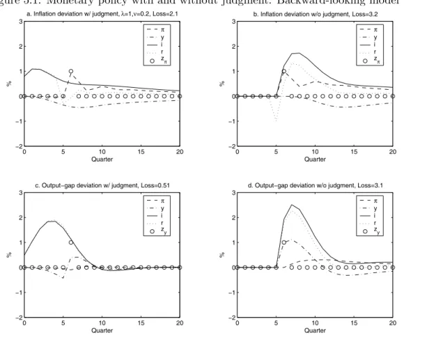
5.1 Backward-looking model 37

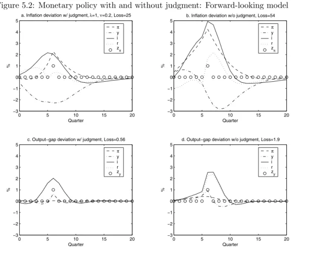
5.2 Forward-looking model 42

5.2.1 Taylor rules 45

6 Conclusions 46

References 48

Appendix 51

Abstract

“Forecast targeting,” forward-looking monetary policy that uses central-bank judgment to construct optimal policy projections of the target variables and the instrument rate, may perform substantially better than monetary policy that disregards judgment and follows a given instrument rule. This is demonstrated in a few examples for two empirical models of the U.S. economy, one forward looking and one backward looking. A practical finite-horizon approximation is used. Optimal policy projections corresponding to the optimal policy under commitment in a timeless perspective can easily be constructed. The whole projection path of the instrument rate is more important than the current instrument setting. The resulting reduced-form reaction function for the current instrument rate is a very complex function of all inputs in the monetary-policy decision process, including the central bank’s judgment. It cannot be summarized as a simple reaction function such as a Taylor rule. Fortunately, it need not be made explicit.

JEL Classification: E42, E52, E58

Non-technical summary

This paper shows that “forecast targeting,” forward-looking monetary policy that uses

central-bank judgment to construct optimal policy projections of the target variables and

the instrument rate, may perform substantially better than monetary policy that disregards

judgment and follows a given instrument rule. This is demonstrated in a few examples for

two empirical models of the U.S. economy, one forward looking and one backward

looking. Furthermore, the paper shows that a complicated infinite-horizon central-bank

projection model of the economy can be closely approximated by a simple finite system

of linear equations, which is easily solved for the optimal policy projections. The optimal

policy projections corresponding to the optimal policy under commitment in a timeless

perspective can then easily be constructed.

The paper emphasizes that the whole projection path of the instrument rate is more

important than the current instrument setting. The resulting reduced-form reaction

function for the current instrument rate is a very complicated function of all inputs in the

monetary-policy decision process, including the central bank's judgment. It cannot be

summarized as a simple reaction function such as a Taylor rule. Fortunately, the reaction

function need not be made explicit. The policymakers only need to ponder the graphs of

the projections of the target variables that are generated in the policy process and choose

the projections of the target variables and the instrument rate that look best, from the

point of view of achieving the central bank's objectives.

On a general level, this paper is motivated by a desire to provide a better theory of

modern monetary policy, both from a descriptive and a normative point of view, than the

one-line modeling of monetary policy common in some of the current literature, such as

“monetary policy is assumed to follow a Taylor rule.” The theory of monetary policy

developed in the paper is arguably better from a descriptive point of view, since it takes

into account some crucial aspects of monetary-policy decisions, such as the collection,

processing, and analysis of large amounts of data, the construction of projections of the

target variables, the use of considerable amounts of judgment, and the desire to achieve

(mostly) relatively specific objectives. The modern monetary-policy process the paper

has in mind can be concisely described as “forecast targeting,” meaning “setting the

instrument rate such that the forecasts of the target variables look good,” where “look

good” refers to the objectives of monetary policy, such as a given target for inflation and

a zero target for the output gap. The paper argues that this view of the monetary-policy

process is also helpful from a normative point of view, for instance, in evaluating the

performance of and suggesting improvements to existing monetary policy.

conditional mean estimate of arbitrary multidimensional stochastic “deviations” – “add

factors” - to the model equations.

1. Introduction

On a general level, this paper is motivated by a desire to provide a better theory of modern

monetary policy, both from a descriptive and a normative point of view, than much of the current

literature on monetary policy. The current literature to a large extent applies a one-line modeling

of monetary policy, such as when the instrument rate is assumed to be a given function of a few

variables, for instance, “monetary policy is assumed to follow a Taylor rule.”

I believe that the theory that I develop here is better from a descriptive point of view, since

it takes into account some crucial aspects of monetary-policy decisions, such as the collection,

processing, and analysis of large amounts of data, the construction of projections of the target

variables, the use of considerable amounts of judgment, and the desire to achieve (mostly) relatively

specific objectives. The modern monetary-policy process I have in mind can be concisely described

as “forecast targeting,” meaning “setting the instrument rate such that the forecasts of the target

variables look good,” where “look good” refers to the objectives of monetary policy, such as a given

target for inflation and a zero target for the output gap.1 I believe this view of the monetary-policy

process is also helpful from a normative point of view, for instance, in evaluating the performance

of and suggesting improvements to existing monetary policy.2

On a more specific level, this paper is motivated by a desire to demonstrate the crucial and

beneficial role of judgment–information, knowledge, and views outside the scope of a particular

model–in modern monetary policy and, in particular, to demonstrate that the appropriate use

of good judgment can dramatically improve monetary-policy performance, even when compared

to policy that is optimal in all respects except for incorporating judgment.3 As will be explained

in detail below, judgment will be represented as the central-bank’s conditional mean estimate of

arbitrary multidimensional stochastic “deviations”–“add factors”–to the model equations.4 I also

1 _{Bernanke [3] discusses and compares forecast targeting (which he refers to as “forecast-based policies”) and}

simple instrument rules (which he refers to as “simple feedback policies”). He states that “the Federal Reserve relies primarily on the forecast-based approach for making policy” and cites Greenspan’s [9] speech, entitled “Risk and Uncertainty in Monetary Policy,” as evidence. He also notes “that not only have most central banks chosen to rely most heavily on forecast-based policies but also that the results, at least in recent years, have generally been quite

good, as most economies have enjoyed low inflation and overall economic stability.”

2

See Svensson [22] and Svensson, Houg, Solheim, and Steigum [28] for examples of evaluations of monetary policy in New Zealand and Norway, respectively, with this perspective.

3

Svensson [25] also emphasizes the role of judgment in monetary policy but does not provide any direct comparision of the performance of monetary policy with and without judgment.

4

wish to demonstrate the benefits of regarding the whole projection paths of the target variables

rather than forecasts at some specific horizon, such as 8 quarters, as the relevant objects in the

monetary-policy decision process. In particular, I believe that it is important to emphasize the whole

projection of future instrument rates rather than just the current instrument rate. Furthermore, the

modern view of the transmission mechanism of monetary policy emphasizes that monetary-policy

actions have effects on the economy and the central bank’s target variables almost exclusively through the private-sector expectations of the future paths of inflation, output, and interest rates

that these actions give rise to; therefore, monetary policy is really the management of private-sector

expectations (Woodford [35]). From this follows that effective implementation of monetary policy requires the effective communication to the private sector of the central bank’s preferred projections, including the instrument-rate projection. The most obvious communication of these projections

is to explicitly announce and motivate them. Finally, I want to demonstrate the benefits of the

approximation of an inherently rather complex infinite-horizon central-bank projection models of

the economy to much simplerfinite-horizon projection models that are much easier to use but still

arbitrarily close approximations to the infinite-horizon models.

The decision process of modern monetary policy has several distinct characteristics (see Brash [4],

Sims [19], and Svensson [22]):

1. Large amounts of data about the state of the economy and the rest of the world, including

private-sector expectations and plans, are collected, processed, and analyzed before each

major decision.

2. Because of lags in the transmission process, monetary-policy actions affect the economy with a lag. For this reason alone, good monetary policy must be forward-looking, aim to influence the

future state of the economy, and therefore rely on forecasts–projections. Central-bank staff

and policymakers make projections of the future development of a number exogenous

vari-ables, such as foreign developments, import supply, export demand,fiscal policy, productivity

growth, and so forth. They also construct projections of a number of endogenous variables,

quantities and prices, under alternative assumptions, including alternative assumptions about

the future path of instrument rates. The policymakers are presented with projections of the

most important variables, including target variables such as inflation and output, often under

alternative assumptions about exogenous variables and, in particular, the instrument rate

3. Throughout this process, a considerable amount of judgment is applied to assumptions and

projections. Projections and monetary-policy decisions cannot rely on models and simple

observable data alone. All models are drastic simplifications of the economy, and data give a

very imperfect view of the state of the economy. Therefore, judgmental adjustments in both

the use of models and the interpretation of their results–adjustments due to information,

knowledge, and views outside the scope of any particular model–are a necessary and essential

component in modern monetary policy.

4. Based on this large amount of information and analysis, the policymakers decide on a current

instrument rate, such that the corresponding projections of the target variables look good

relative to the central bank’s objectives. Since the projections of the target variables depend

insignificantly on the current instrument-rate setting and mainly on the whole path of future

instrument rates, the policymakers, explicitly or implicitly, actually choose an

instrument-rate projection–an instrument-instrument-rate plan–and the current instrument-instrument-rate decision can be

seen as the first element of that plan.

5. Finally, the current instrument rate is announced and implemented. In many cases, the

corresponding projections for inflation and output or the output gap are also announced. In

a few cases, an instrument-rate projection is announced as well.5

This process makes the current instrument-rate decision a very complex function of the large

amounts of data and judgment that have entered into the process. I believe that it is not very helpful

to summarize this function as a simple reaction function such as a Taylor rule. Furthermore, the

resulting complex reaction function is areduced form, which depends on the central-bank objectives,

its view of the transmission mechanism of monetary policy, the data the central bank has collected,

and the judgment it has exercised. It is the endogenous complex result of a complex process. In

no way is this reaction function structural, in the sense of being invariant to the central bank’s

view of the transmission mechanism and private-sector behavior, or the amount of information and

judgmental adjustments. Still, much current literature treats monetary policy as characterized by

a given reaction function that is essentially structural and invariant to changes in the model of the

economy. Treating the reaction function as a reduced form is a first step in a sensible theory of

5 _{The Reserve Bank of New Zealand has published an instrument-rate projection for many years. The Bank of}

monetary policy. But, fortunately, this complex reduced-form reaction function need not be made

explicit. It is actually not needed in the modern monetary-policy process.

However, there is a convenient, more structural representation of monetary policy, namely in

the form of a targeting rule, as advocated recently in some detail in Svensson and Woodford [30]

and Svensson [25] and earlier more generally in Svensson [21]. An optimal targeting rule is afi

rst-order condition for optimal monetary policy. It corresponds to the standard efficiency condition of equality between the marginal rates of substitution and the marginal rates of transformation

between the target variables, the former given by the monetary-policy loss function, the latter

given by the transmission mechanism of monetary policy. An optimal targeting rule is invariant to

everything else in the model, including additive judgment and the stochastic properties of additive

shocks. Thus, it is a compact, robust, and structural representation of monetary policy, and

much more robust than the optimal reaction function. A simple targeting rule can potentially

be a practical representation of robust monetary policy, a robust monetary policy that performs

reasonably well under different circumstances.6

Optimal targeting rules remain a practical way of representing optimal monetary policy in the

small models usually applied for academic monetary-policy analysis. However, for the larger and

higher-dimensional operational macromodels used by many central banks in constructing

projec-tions, the optimal targeting rule becomes more complex and arguably less practical as a

representa-tion of optimal monetary policy. In this paper, it is demonstrated that optimal policy projecrepresenta-tions,

the projections corresponding to optimal policy under commitment in a timeless perspective, can

easily be derived directly with simple numerical methods, without reference to any optimal

target-ing rule.7 For practical optimal monetary policy, policymakers actually need not know the optimal

targeting rule. Even less do they need to know any reaction function. They only need to ponder

the graphs of the projections of the target variables that are generated in the policy process and

choose the projections of the target variables and the instrument rate that look best relative to the

central bank’s objectives.

The paper is organized in the following way. Section 2 lays out a reasonably general infi

nite-horizon model of the transmission mechanism and the central bank’s objectives; defines projections,

judgment and optimal policy projections; and specifies how the optimal policy can be implemented

6

McCallum and Nelson [15] have recently criticized the advocacy of targeting rules in Svensson [25]. Svensson [26] rebuts this criticism and gives references to a rapidly growing literature that applies targeting rules to monetary-policy analysis. Walsh [34] shows a case of equivalence between targeting rules and robust control.

7 _{Nevertheless, a general form of an optimal targeting rule is derived in appendix F, for thefinite-horizon}

and what information the private sector needs from the central bank. The section also presents a

simple model of judgment, when the deviation is a version of a finite-order moving average. Then

judgment can be seen as the accumulation of information over time and allows for a recursive

but high-dimensional representation of the dynamics of the deviation and judgment. Finally, the

section represents the optimal policy projections as the solution to a somewhat complex system of

difference equations, while taking judgment into account. It also makes the point that, fortunately, the complex reduced-form reaction function need not be made explicit. Section 3 presents a

conve-nientfinite-horizon model for the construction of optimal policy projections, for both forward- and

backward-looking models. Thisfinite-horizon model can be written as a simplefinite system of

lin-ear equations. Nevertheless, it is an exact or arbitrarily close approximation to the infinite-horizon

model and is easily solved for the optimal policy projections taking judgment into account. Section

4 discusses and specifies monetary policy that disregards judgment and follows different instrument rules, such as variants of the Taylor rule or more complex instrument rules that are optimal in the

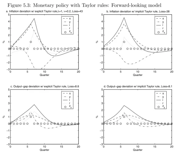
absence of judgment. Section 5 gives examples of and compares monetary policy with and without

judgment, for two different empirical models of the U.S. economy: the backward-looking model of Rudebusch and Svensson [18] and the forward-looking New Keynesian model of Lindé [13]. In

these examples, monetary policy with judgment results in substantially better performance than

monetary policy without judgment. This is also the case when monetary policy without judgment is

represented as a Taylor rule where the instrument rate responds to forward-looking variables that

incorporate private-sector judgment (although, as emphasized below, there are serious principal

and practical problems in implementing such an instrument rule). Section 6 presents conclusions.

A separate and extensive appendix contains numerous technical details.8 These include a general

solution of the policy problem and the related system of difference equations with forward-looking variables when the deviation is an arbitrary stochastic process; a specification of the model when

the deviation and judgment are finite-order moving-average processes and the application of the

practical method of Marcet and Marimon [14] to that case; the precise mathematical structure of

the finite-horizon approximation model, including the optimal targeting rule; and details on the

empirical backward- and forward-looking models.

8 _{The appendix is available at www.princeton.edu/}

2. A model of the policy problem with judgment

Consider the following linear model of an economy with a private sector and a central bank,9 in a

form that allows for both predetermined and forward-looking variables as well as judgment,

∙ Xt+1

Cxt+1|t

¸

=A ∙

Xt

xt

¸

+Bit+

∙ zt+1

0

¸

. (2.1)

Here, Xt is a (column) nX-vector of predetermined variables (one of these may be unity to

con-veniently incorporate constants in the model) in period t; xt is an nx-vector of forward-looking

variables; it is an ni-vector of central-bank instruments (the forward-looking variables and the

instruments are the nonpredetermined variables); zt is an exogenous nX-vector stochastic process

and called thedeviation in period t; and A,B, andC are matrices of the appropriate dimension.

For any variableqt, I let qt+τ|t denote private-sector expectations of the realization in periodt+τ

of qt+τ conditional on private-sector information available in period t. I assume that the private

sector has rational expectations, given its information.

For increased generality, the model is formulated in terms of an arbitrary number of instruments,

ni. In most practical applications, monetary policy can be seen as having only one instrument–a

short interest rate, the instrument rate–so thenni = 1.

The upper block of (2.1) providesnX equations determining thenX-vectorXt+1in periodt+ 1

for given Xt,xt,it and zt+1,

Xt+1 =A11Xt+A12xt+B1it+zt+1, (2.2)

whereA and B are partitioned conformably withXt and xt as

A_≡

∙

A11 A12

A21 A22

¸

, B _≡

∙ B1

B2

¸

. (2.3)

The realization of the deviation and the predetermined variables in each period occurs and is

observed by the private sector and the central bank in the beginning of the period (the realization

of zt+1 can be inferred from Xt+1,Xt,xt and it and (2.2)).10

The lower block of (2.1) providesnxequations determining thenx-vectorxtin periodtfor given

x_t+1|t,Xt, and it,

xt=A−221(Cxt+1|t−A21Xt−B2it); (2.4)

9 _{For simplicitly, there is no explicitfiscal authority in the model, but such an authority and its behavior can be}

included in the model (2.1).

1 0 _{See Svensson and Woodford [29] for an analysis of optimal policy in a model with forward-looking variables}

I hence assume that the nx×nx submatrix A22 is invertible. The realization ofXt is observed by

the private sector and the central bank in the beginning of periodt; the central bank then sets the

instruments, it; after observing the instruments, the private sector forms its expectations, xt+1|t;

and this finally determines the forward-looking variables xt.

To assume that the deviation appears only in the upper block of (2.1) is not restrictive. Suppose

that I have a model where the deviation appears in both blocks,

∙ X_to₊₁ Cxt+1|t

¸

=

∙

Ao₁₁ Ao₁₂ Ao₂₁ Ao₂₂

¸∙ X_to

xt

¸

+

∙ B₁o B₂o

¸

it+

∙ z₁o_,t+1

z₂o_,t

¸

,

By adding the vectorz_to to the predetermined variables, I can always form a new model of the form

(2.1), where

Xt≡

∙ X_to

z₂o_t

¸

, A_≡

⎡ ⎣ A

o

11 0 Ao12

0 0 0

Ao₂₁ 0 Ao₂₂ ⎤

⎦, B _≡

⎡ ⎣ B

o 1

0

B₂o ⎤

⎦, zt≡

∙ zo_1t

z₂o

¸

,

and there is no deviation in the lower block.

As in Svensson [25], the deviation represents additional determinants–determinants outside

the model–of the variables in the economy, the difference between the actual value of a variable and the value predicted by the model. It can be interpreted as model perturbations, as in the

literature on robust control.11 The central bank’s mean estimate of future deviations will be

identified with the central bank’sjudgment. It represents the unavoidable judgment always applied

in modern monetary policy. Any existing model is always an approximation of the true model

of the economy, and monetary-policy makers always find it necessary to make some judgmental

adjustments to the results of any given model. Such judgmental adjustments could refer to future

fiscal policy, productivity, consumption, investment, international trade, foreign-exchange and other

risk premia, raw-material prices, private-sector expectations, and so forth. The “add factors”

applied to model equations in central-bank projections (Reifschneider, Stockton, and Wilcox [17])

are an example of central-bank judgment. Given this interpretation of judgment and the deviation

zt+1, it would be completely misleading to make a simplifying assumption such as the deviation

being a simple autoregressive process. In that case, it could just be incorporated among the

predetermined variables. Thus, I will refrain from such an assumption and instead leave the dynamic

properties of zt+1 unspecified, except in a special case when the deviation is a version of a fi

nite-order moving-average process. Generally, the focus will be on the central bank’s judgment of the

whole sequence of future deviations.

1 1 _{See, for instance, Hansen and Sargent [10]. However, that literature deals with the more complex case when the}

More precisely, let the infinite-dimensional period-trandom vectorζt_≡(z_t0₊₁, z_t0₊₂, ...)0 (where0

denotes the transpose) denote the vector of the (in periodt) unknown random vectorszt+1,zt+2,...

Let the central bank’s beliefs in periodtabout the random vectorζtbe represented by the infi

nite-dimensional probability distribution Φt with distribution function Φt(ζt). The probability

distri-bution Φt may itself be time-varying and stochastic. The central bank is assumed to know the

matrices A,B,C, D, and W and the discount factor δ (D, W, and δ refer to the central bank’s

objectives and are defined below). The private sector is assumed to know the matrices A,B, and

C, but may or may not know the central bank’s objectives (that is, D, W, and δ). The private

sector may or may not have the same beliefs about the future deviations as the central bank.

Let Yt be an nY-vector of target variables. For simplicity, these target variables are measured

as the difference from afixednY-vectorY∗ oftarget levels. This vector of target levels is heldfixed

throughout this paper. In order to examine the consequences of shifting target levels, one only

needs to replaceYt _{by Y}t_−Y∗ _{throughout the paper. Let the target variables be given by}

Yt=D

⎡ ⎣

Xt

xt

it

⎤

⎦, (2.5)

whereD is annY ×(nX+nx+ni) matrix.

Let the central bank’s intertemporal loss function in periodt be

Et ∞

X

τ=0

δτLt+τ ≡

Z _X∞

τ=0

δτLt+τdΦt(ζt), (2.6)

where0< δ_≤1 is a discount factor,Lt is the period loss given by

Lt= 1 2Y

0

tW Yt, (2.7)

and W is a symmetric positive semidefinitenY ×nY matrix. That is, in periodt the central bank

wants to minimize the expected discounted sum of current and future losses, where the expectation

Et is with respect to the distributionΦt.

Since this is a linear model with a quadratic loss function and the random deviations enter

addi-tively, the conditions for certainty equivalence are satisfied. Then, as shown in detail in appendix A,

the optimal policy in periodt need only consider central-bank mean forecasts–projections–of all

variables, including the infinite-dimensional mean forecast, zt, of the random vectorζt,

zt_≡Etζt≡

Z

The central-bank projection in period t of the realization of the deviation in period t+τ,zt+τ, is

denoted zt+τ ,t, so zt ≡ (zt0+1,t, zt0+2,t, ...)0. The projection zt is identified with the central bank’s

judgment. Under the assumed certainty equivalence, the projection zt is, for optimal policy, a

sufficient statistic for the distribution Φt. Although there is genuine uncertainty about the future

random deviations, ζt, the only thing that matters for policy is the mean, the judgment, zt. The

second and higher moments of ζt–the variance, skew, kurtosis, and so forth–do not matter for

policy.12 The judgment can itself be seen as an exogenous infinite-dimensional random vector that

is realized in the beginning of each period and summarizes the central bank’s relevant information

in that period about expected future deviations.

Let qt_≡(q_t,t0 , q_t0_+1,t, ...)0 denote a central-bank projection in period tfor any vector of variables

qt+τ (τ ≥ 0) (with the exception of εt and εt+τ ,t, to be introduced below), a central-bank mean

forecast conditional on central-bank information in period t. (Thus, for variables other than the

deviation, the projection also includes also the current value, qt,t = qt.) The central bank then

constructs various projections of the endogenous variables to be used in its decision process. These

projections of endogenous variables may be conditional on various assumptions. In order to keep

private-sector expectations and central-bank projections conceptually distinct, I denote the former

by q_t+τ|t and the latter byqt+τ ,t for any variable qt.

For given judgment, zt, the projection model of the central bank for the projections (Xt, xt,

it_{, Y}t_{) in periodt–the model the central bank uses in the decision process to consider alternative}

projections–will be

∙

Xt+τ+1,t

Cxt+τ+1,t

¸

=A ∙

Xt+τ ,t

xt+τ ,t

¸

+Bit+τ ,t+

∙

zt+τ+1,t 0

¸

, (2.8)

Yt+τ ,t=D

⎡ ⎣

Xt+τ ,t

xt+τ ,t

it+τ ,t

⎤

⎦ (2.9)

forτ _≥0, whereXt,t satisfies

Xt,t=Xt, (2.10)

since the realization of the predetermined variables is assumed to be observed in the beginning of

period t.

In order to introduce more compact notation, let the (nX+nx+ni)-vectorst≡(Xt0, x0t, i0t)0denote

the state of the economy in period t, and let the vector st+τ ,t ≡(Xt0+τ ,t, x0t+τ ,t, i0t+τ ,t)0 denote the

1 2

projection in periodtof the state of the economy in periodt+τ. Finally, let the infinite-dimensional

vectorst_≡(s0_t,t, s0_t+1,t, st+2,t, ...)0 denote a projection in periodt of the (current and future) states

of the economy. By (2.9), I can write the projection of the target variables in a compact way, as a

linear function of the projection of the states of the economy, as

Yt= ˜Dst, (2.11)

whereD˜ is an infinite-dimensional block-diagonal matrix with theτ+ 1-th diagonal block equal to

D forτ _≥0.

The set of feasible projections of the states of the economy in periodt, _St, can now be defined

as the set of projections st that satisfy (2.8)-(2.10) for given Xt and zt.

The intertemporal loss function (2.6) with (2.7) induces an intertemporal loss function for the

target-variable projection,13

L(Yt)_≡ ∞

X

τ=0

δτY_t0_{+τ ,t}W Yt+τ ,t, (2.12)

The policy problem in period t is to find the optimal policy projection (ˆst,Yˆt), the projection

that minimizes (2.12) over the set of feasible projections of the states of the economy, that is,

subject to (2.8)-(2.11) forτ _≥0 for given Xt and zt. More compactly,

ˆ

st= arg min st_∈StL( ˜Ds

t_{), (2.13)}

ˆ

Yt _{≡ D}˜_{sˆ; and the optimal policy projection ( ˆX}t_,xˆt_,ˆıt_{) of the predetermined variables,}

forward-looking variables, and instruments can be extracted from ˆst.

The policy problem will be further specified below to correspond to commitment in a “timeless

perspective,” in order to avoid any time-consistency problems (see Woodford [36] and Svensson and

Woodford [30]).

2.1. Implementation and what information the private sector needs

The implementation of the optimal policy in period t involves announcing the optimal policy

projection and setting the instruments in period t equal to the first element of the instrument

projection,

it= ˆıt,t.

1 3 _{Note that min E}

tS∞_τ=0δτLt+τ = min{L(Yt) + EtS∞_τ=0δτ(Yt+τ −Yt+τ ,t)0W(Yt+τ−Yt+τ ,t)}= min{L(Yt) + S∞

τ=0δ

τ

trace(WCovtYt+τ)}. By certainty equivalence, CovtYt+τ ≡Et(Yt+τ −Yt+τ ,t)(Yt+τ −Yt+τ ,t)0 ≡ U

(Yt+τ−

Yt+τ ,t)(Yt+τ−Yt+τ ,t)0dΦt(ζt) is independent of policy, so minimizing (2.12) in periodtimplies the same policy as

minimizing (2.6) in periodt.

Furthermore, note that, since trace(WCovtYt+τ) will normally be strictly positive, (2.6) will normally converge

In period t+ 1, conditional on new realizations of the predetermined variables, Xt+1, and the

judgment, zt+1, a new optimal policy projection,( ˆXt+1,xˆt+1,ˆıt+1,Yˆt+1), is found and announced

together with a new instrument setting,

it+1= ˆıt+1,t+1.

In a forward-looking model, the private sector (including policymakers other than the central

bank) will need to know at least parts of the aggregate projectionsXˆt,xˆt, andˆıt, in order to make

decisions consistent with these and make the rational-expectations equilibrium in the economy

correspond to the central bank’s optimal policy projection. If the private sector knows the matrices

A, B,C,D, and W and the discount factor δ and has the same judgment zt as the central bank,

it can in principle compute the optimal policy projection itself–assuming that it has the same

computational capacity as the central bank.

However, the private sector actually needs to know less. An assumption maintained through

this paper is that the private sector knows the model (2.1), in the sense of knowing the matrices

A,B, and C. Furthermore, it observes Xt (determined byXt−1,xt−1, andit−1 in period t−1 and

the realization ofzt in the beginning of periodtaccording to (2.2)) in the beginning periodt, then

observesit= ˆıt,tset by the central bank, thereafter forms one-period-ahead expectationsxt+1|t, and

finally determines (and thereby knows) xt; after this, period tends. In order to make decisions in

periodtconsistent with the optimal policy projection–that is, decisions resulting inxt= ˆxt,tfrom

(2.4)–the private sector needs be able to form expectationsx_t+1|t= ˆxt+1,t. The most direct way is if

the central bank announcesxˆt+1,tand the private sector believes the announcement. Formally,xˆt+1,t

is the minimum additional information the private sector needs. However, the central bank may

have to provide the whole optimal policy projection, and also motivate the underlying judgment,

in order to demonstrate the optimal policy projections are internally consistent with the model

(2.1). In particular, the private sector may not believexˆt+1,t unless it is apparently consistent with

the whole projectionˆıt_{. Furthermore, the private sector will need to know the central bank’s loss}

function–D, W, and δ–in order to judge whether the projections announced are really optimal

relative to the central bank’s loss function and thereby incentive-compatible, credible. Only then

may the central bank be able to convince the private sector to form expectations according to

the optimal policy projection.14 _{Indeed, the private sector completely trusting the central bank’s}

1 4 _{Being explicit about the loss function and announcing the optimal policy projection also seem to take care of}

problem discussed below.15 16

2.2. Judgment as a finite-order moving average

Consider the special case when the deviation is a version of a moving-average stochastic process

with a given finite orderT >0 (whereT could be relatively large),

zt+1 =εt+1+

T

X

j=1

εt+1,t+1−j, (2.14)

where˜εt≡(ε0t, εt0)0≡(ε0t, ε0t+1,t, ..., ε0t+T,t)0 is a zero-mean iid random(T+ 1)nX-vector realized in

the beginning of period t and called the innovation in period t.17 _{For T = 0, z}

t+1 is a simple iid

disturbance. ForT >0, the deviation is a version of a moving-average process.

It follows that the central-bank judgment zt+τ ,t (τ ≥1) is also a finite-order moving average

and satisfies

zt+τ ,t ≡Etzt+τ = T

X

j=τ

εt+τ ,t+τ−j =εt+τ ,t+ T

X

j=τ+1

εt+τ ,t+τ−j =εt+τ ,t+zt+τ ,t−1.

Hence, εt+τ ,t = zt+τ ,t−zt+τ ,t−1 can be interpreted as the innovation in period t to the previous

judgment zt+τ ,t−1, the new information the central bank receives in period tabout the realization

of zt+τ in periodt+τ. Hence, the judgment zt+τ ,t in periodt is the sum of current and previous

information about zt+τ. For horizons larger than T, the central-bank judgment is constant and,

without loss of generality, equal to zero,

zt+τ ,t= 0 (τ > T). (2.15)

The dynamics of the deviation zt and the judgment zt+1 can then be written as

∙ zt+1

zt+1

¸

=Az

∙ zt

zt

¸

+

∙ εt

εt+1

¸

, (2.16)

where the (T+ 1)nX×(T+ 1)nX matrix Az is defined as

Az ≡

⎡ ⎣

0nX×nX InX 0nX×(T−1)nX

0(T−1)nX×nX 0(T−1)nX×nX I(T−1)nX

0nX×nX 0nX×nX 0nX×(T−1)nX ⎤ ⎦,

1 5 _{See Geraats [7] for such examples.}

1 6 _{In a much noted contribution, Morris and Shin [16] and Amato, Morris, and Shin [1] have emphasized the}

pos-sibility that public information may be bad and reduce social welfare by crowding out private information. Svensson [27] scrutinizes this results and shows that, in the model considered by Morris and Shin, public information actually increases social welfare for reasonable parameters.

1 7

Note thatεt_≡(ε0t+1,t, εt0+2,t, ..., ε0t+T ,t)0here denotes a random vector realized in the beginning of periodtand

not the projection in periodtof the random variables εt+1,εt+2, ...,εt+T. That projection is always zero under the

above assumption ofεt _{being a zero-mean iid random variable.}

where0m×nandImdenote anm×nzero matrix and ann×nidentity matrix, respectively. Thus, the

dynamics of the deviation and the judgment has a convenient linear and recursive representation.

The modeling of the dynamics of the deviation, zt, and the additive judgment, zt, in (2.16)

allows for a relatively flexible accumulation of information about future deviations. Whereas the

stochastic process for the deviation is not a simple Markov process in terms of itself but afinite-order

moving-average process, it can be written as a higher-dimensional AR(1) process. The restriction

imposed is that the innovation is zero-mean and iid across periods. There is no restriction of

the variance and covariance of the elements of ˜εt within the period. It follows that, for instance,

εt+τ ,t may have a variance that is decreasing inτ, corresponding to a situation where there is less

information about the mean projection of deviations further into the future; by assumption, there

is no specific information about the deviation forτ > T. For givent, there may be serial correlation

of εt+τ ,t across τ, corresponding to new information about serially correlated future deviations.

2.3. Representing optimal policy projections

Without the judgment terms (or, alternatively, with the deviation being an iid zero-mean process

or an autoregressive process with iid shocks), the above infinite-horizon linear-quadratic problem

with forward-looking variables is a well-known problem, examined and solved in Backus and Driffill [2], Currie and Levine [5], and Söderlind [20]. The traditional way tofind a solution to this problem

is to derive the first-order conditions for an optimum and combine the first-order conditions with

the model (2.1) to form a system of difference equations with an infinite horizon. The solution can then also be expressed as a difference equation. Furthermore, Marcet and Marimon [14] have shown a new practial way of reformulating the problem with forward-looking variables as a recursive

saddlepoint problem (see appendix D).

A new element here is the solution with the judgment. For the case when the deviation is afi

nite-order moving average, the dynamics of the deviation and the judgment, (2.16), can be incorporated

with (2.1), the vector of predetermined variables can be expanded to includezt, and the standard

solution can be applied directly.18 The details for this case are provided in appendices C and D.

When the judgment is a realization of an infinite-dimensional random vector, the standard solution

has to be modified to take that into account. The details of that solution in the form of a difference equation are explained in appendices A and B. Here I shallfirst report the solution in the form of

an infinite-horizon difference equation and later develop a very convenient finite-horizon version of

1 8 _{Sincezt is incorporated inXt, one does not need to addzt as a separate predetermined variable.}

Under the assumption of optimization under commitment, one way to describe the optimal

policy projection is by the following difference equations,

∙

ˆ

xt+τ ,t ˆıt+τ ,t

¸

= F

⎡ ⎣

ˆ

Xt+τ ,t

zt+τ ,t

Ξt+τ−1,t

⎤

⎦, (2.17)

∙ _ˆ Xt+τ+1,t

Ξt+τ ,t

¸

= M

⎡ ⎣

ˆ

Xt+τ ,t

zt+τ ,t

Ξt+τ−1,t

⎤

⎦, (2.18)

forτ _≥0, whereXˆt,t=Xt. When the deviation is afinite-order moving average and the judgment is

finite-dimensional,zt+τ ,tdenotes theT nX-vector(zt0+τ+1,t, zt0+τ+2,t, ..., z0t+τ+T,t)0, wherezt+τ+j,t = 0

for j+τ > T. When the judgment is infinite-dimensional, zt+τ ,t denotes the infinite-dimensional

vector (z_t0_+τ+1,t, z_t0_+τ+2,t, ...)0. In the former case, F and M are finite-dimensional matrices. In

the latter case, F and M include a linear operator R on zt+τ ,t (an infinite-dimensional matrix) of

the form P∞_j=0Rjzt+1+τ+j,t, where {Rj}∞j=0 is a sequence of matrices. The matrices F, M, and

{Rj}∞j=0 depend on A, B, C, D, W, and δ, but they are independent of the second and higher

moments of the deviation. The nX-vector Ξt+τ ,t consists of the Lagrange multipliers of the lower

block of (2.8), the block determining the projection of the forward-looking variables.

As discussed in appendix A, the value of the initial Lagrange multiplier,Ξt−1,t, is zero, if there is

commitment from scratch in periodt, that is, disregarding any previous commitments. This reflects

a time-consistency problem when there is reoptimization and recommitment in later periods, as

is inherently the case in practical monetary policy. Instead, I assume that the optimization is

under commitment in a timeless perspective. Then, if the optimization, and reoptimization, under

commitment in a timeless perspective started in an earlier period and has occurred since then, the

initial value of the Lagrange multiplier satisfies

Ξt−1,t=Ξt−1,t−1, (2.19)

whereΞt−1,t−1 denotes the Lagrange multiplier of the lower block of (2.8) for the determination of

xt−1,t−1 in the decision problem in periodt−1. The dependence of the optimal policy projection

in periodton this Lagrange multiplier from the decision problem in the previous period makes the

optimal policy projection depend on previous projections and illustrates the history dependence of

It follows from (2.17)-(2.19) and (2.11) that the optimal policy projection of the states of the

economy, the target variables, and the instruments will be linear functions ofXt,zt, and Ξt−1,t−1,

which can be written in a compact way as

ˆ

st=H ⎡ ⎣

Xt

zt

Ξt−1,t−1

⎤

⎦, Yˆt= ˜DH ⎡ ⎣

Xt

zt

Ξt−1,t−1

⎤

⎦, ˆıt=Hi

⎡ ⎣

Xt

zt

Ξt−1,t−1

⎤

⎦, (2.20)

whereH is an appropriately formed infinite-dimensional matrix, and Hi is an infinite-dimensional

submatrix ofH consisting of the rows corresponding to the instruments. In particular, the

instru-ment setting in periodt will be given by

it= ˆıt,t=h

⎡ ⎣

Xt

zt

Ξt−1,t−1

⎤

⎦, (2.21)

where the finite- or infinite-dimensional matrixhconsists of the ni first rows of the matrix Hi.

As explained in Svensson and Woodford [30], a simple way of imposing the timeless perspective

is to add a term to the intertemporal loss function (2.12),

L(Yt) +Ξt−1,t−1

1

δCxt,t. (2.22)

In the policy problem in period t₋1,Ξt−1,t−1C can be interpreted as the marginal loss in period

t₋1 of a change in the one-period-ahead projection of the forward-looking variables, xt,t−1. The

time-consistency problem arises from disregarding that marginal loss in the policy problem in

period t. Adding the corresponding term to the loss function in period t as in (2.22) handles the

time-consistency problem, and the optimal policy under commitment in the timeless perspective

will result from minimizing (2.22) subject to (2.8)-(2.10) for givenXt,zt, andΞt−1,t−1.19 Sincext,t

is an element of the projectionst, the optimal policy projectionsˆt is then defined as

ˆ

st= arg min st_∈S t

{L( ˜Dst) +Ξt−1,t−1

1

δCxt,t}, (2.23)

for given Xt,zt, and Ξt−1,t−1.

From (2.18) follows that the Lagrange multiplier Ξt,t, to be used in the decision problem in

period t+ 1, will be given by

Ξt,t=HΞ ⎡ ⎣

Xt

zt

Ξt−1,t−1

⎤

⎦, (2.24)

1 9

Alternatively, as discussed in Giannoni and Woodford [8] and Svensson and Woodford [30], one can impose the constraint

xt,t=Fx %

Xt zt Ξt−1,t−1

& ,

where F in (2.17) is suitably partitioned. In the present context, it is more practical to add the term to the

whereHΞ is afinite- or infinite-dimensional matrix.

Let theset of feasible target-variable projections in periodt,_Yt, be defined as the set of

target-variable projections satisfying (2.11) for projections st in the set St for given Xt and zt. In the

special case where the forward-looking variables, xt, happen to be target variables and elements

inYt, so xt,t is an element of Yt, the optimal target-variable projection, Yˆt, can be defined as the

target-variable projectionYtthat minimizes (2.22) on the set _Yt, for given Xt,zt, andΞt−1,t−1,

ˆ

Yt= arg min Yt_∈Y

t{L

(Yt) +Ξt−1,t−1

1

δCxt,t}.

However, in the more general case when some or all forward-looking variables are not target

vari-ables,xt,tis not an element ofYt, and the optimal policy projection has to be found by optimization

over the set _St, as in (2.23).

2.4. Backward-looking model

In a backward-looking model, there are no forward-looking variables: nx = 0. There is no lower

block in (2.1) and (2.8), and there are no forward-looking variables in (2.5) and (2.9). There are

no projections of forward-looking variables and Lagrange multipliers in (2.17), (2.18), (2.20), and

(2.21). There is no time consistency problem and no need to consider commitment in a timeless

perspective.

Hence, for a backward-looking model, the optimal target-variable projection can always be

found by minimizing (2.12) over the set of feasible target-variable projections,

ˆ

Yt= arg min Yt_∈Y t

L(Yt),

for given Xt and zt.

2.5. The complex reduced-form reaction function need not be made explicit

The compact notation for the determination of the period-tinstrumentitin (2.21) and the Lagrange

multiplier Ξt,t in (2.24) may have given the impression that optimal monetary policy is just a

matter of calculating thefinite- or infinite-dimensional matriceshandHΞonce and for all; then, in

each period, first observe Xt, form zt, and recall Ξt−1,t−1 from last period’s decision; then simply

compute, announce, and implement it from (2.21); and finally compute Ξt,t to be used in next

This is a misleading impression, though. First,handHΞare indeed high- or infinite-dimensional

and therefore difficult to grasp and interpret. Second, zt is also high- or infinite-dimensional. It is difficult to conceive of policymakers or even staff pondering pages and pages, or computer screens and computer screens, of huge arrays of numbers in small print, arguing and debating

about adjustments of the numbers ofzt, such as the numbers in rows 220—250 and 335—385. Third,

no central bank (certainly no central bank that I have any more thorough information about)

behaves in that way, and is ever likely to behave that way. Instead, the practical presentation

of information and options to policymakers is always in the form of multiple graphs, modest-size

tables, and modest amounts of text.

Fourth, the intertemporal loss function _L(Yt) has the projections of the target variables as its

argument. What matters for the construction of the target variables is the whole projection path

of the instruments, not the current instrument setting. The obvious conclusion is that the relevant

objects of importance in the decision process are the whole projection paths of the target variables

and the instruments, not the current instrument setting or projections of the target variables at some

fixed horizon. These projection paths are most conveniently illustrated as graphs. Indeed, graphs of

projections are prominent in the existing monetary-policy reports where projections are reported.

The analytical techniques discussed in this paper should predominantly be seen as techniques for

computer-generated graphs of whole projection paths. Pondering such graphs is an essential part

of the monetary-policy decision process. Importantly, policymakers need not know the underlying

detailed high- or infinite-dimensional matrices behind the construction of those graphs. Therefore,

the complex reduced-form reaction functions embedded in these matrices need not be made explicit.

Fifth, in the discussion in section 2.1, there was no reference to the reaction function, only to

the optimal policy projection. Given Xt and it, the private sector needs to be able to form the

expectations xt+1|t in order to make decisions in period t. The minimum for this is the central

bank’s announcement of xˆt+1,t. In order to make that announcement credible, the central bank

may have to announce the complete optimal policy projection and motivate its judgment. But it

does not need to announce any reaction function. In principle, given the reaction function, the

private sector could combine the reaction function with the model and solve for the optimal policy

3. A

fi

nite-horizon projection model

Regardless of whether the judgment is finite- or infinite-dimensional (that is, whether (2.15) holds

or not), the problem of minimizing the intertemporal loss function is an infinite-horizon problem.

From a practical and computational point of view, it is convenient to transform the infinite-horizon

policy problem above to afinite-horizon one. When the judgment satisfies (2.15), this can be done

in a simple and approximate, but arbitrarily close to exact, way for the forward-looking model, and

in a simple and exact way for the backward-looking model. The finite-horizon model also makes

it very easy to incorporate any arbitrary constraints on the projections, for instance, a particular

form of the instrument projection, such as a constant instrument for some periods. Then, all the

relevant projection paths are computed in one simple step.

3.1. Forward-looking model

Suppose that the estimate of the deviation is constant beyond a fixed horizon T. Without loss of

generality, assume that the constant is zero.20 That is, I assume (2.15).

Start by writing the projection model (2.8) and (2.10) for τ = 0, ..., T ₋1 as

Xt,t = Xt, (3.1)

−As˜ t+τ ,t+

∙

Xt+τ+1,t

Cxt+τ+1,t

¸

=

∙

zt+τ+1,t 0

¸

(τ = 0, ..., T₋1). (3.2)

whereA˜is the(nX+nx)×(nX+nx+ni) matrix defined byA˜≡[A B]. ThefirstnX equations of

the last block ofnX+nx equations in (3.2) determineXt+T,tfor givenXt+T−1,t,xt+T−1,t,it+T−1,t,

and zt+T,t. The last nx equations of that block are

−A21Xt+T−1,t−A22xt+T−1,t−B2it+T−1,t+Cxt+T,t= 0.

They determine xt+T−1,t for given Xt+T−1,t and it+T−1,t, and, importantly, for given xt+T,t. A

problem is thatnxequations determiningxt+T,tare lacking. I will assume thatxt+T,tis determined

by the assumption thatxt+T+1,tis equal to its steady-state level. That is, I assume that the optimal

policy projection has the property that, for (2.15), it approaches a steady state whenT _{→ ∞}. This

is true for the models and loss functions considered here. Without loss of generality, I assume that

the steady-state values for the forward-looking variables are zero,

xt+T+1,t= 0. (3.3)

2 0

If the estimate of the deviation from horizon T on is constant but nonzero, it can be incorporated among

other constants in the model. If the estimate of the deviation from horizon T on is not constant but follows an

From this follows thatXt+T,t,xt+T,t, andit+T,tmust satisfy

−A21Xt+T,t−A22xt+T,t−B2it+T,t= 0, (3.4)

which gives me the desirednx equations for xt+T,t.

Letst, the projection of the states of the economy, now denote thefinite-dimensional (T+ 1)_×

(nX +nx+ni)-vector st ≡(s0t,t, st0+1,t, ..., s0t+T,t)0. Similarly, let all projections qt for q =X, x,i

and Y now denote the finite-dimensional vector qt _≡(q0_t,t, q_t0_+1,t, ..., q_t0_+T,t)0. Finally, let zt be the

T nX-vectorzt≡(zt0+1,t, zt0+2,t, ..., zt0+T,t)0 (recall thatztdoes not include the component zt).

The finite-horizon projection model for the projection of the states of the economy, st, then

consists of (3.1), (3.2) and (3.4). It can be written compactly as

Gst=gt, (3.5)

whereGis the (T+ 1)(nX+nx)×(T+ 1)(nX+nx+ni) matrix formed from the matrices on the

left side of (3.1), (3.2), and (3.4), and gt is a (T + 1)(nX+nx)-vector formed from the right side

of (3.1), (3.2), and (3.4) as gt _≡ (X_t0, z_t0_+1,t,00, z0_t+2,t,00, ..., z0_t+T,t,00,00)0 (where zeros denote zero

vectors of appropriate dimension).

Since Yt now denotes the finite-dimensional (T + 1)nY-vector Yt ≡ (Yt,t0 , Yt0+1,t, ..., Yt0+T,t)0, I

can write

Yt= ˜Dst, (3.6)

whereD˜ now denotes afinite-dimensional (T+ 1)nY ×(T+ 1)(nX+nx+ni)block-diagonal matrix

with the matrix Din each diagonal block.

The set of feasible projections, _St, is then defined as thefinite-dimensional set ofstthat satisfy

(3.5) and (3.6) for a givengt, that is, for a given Xtand zt.

It remains to specify the intertemporal loss function in the forward-looking model in thefi

nite-horizon case. In the forward-looking model, under assumption (2.15), the minimum loss from the

horizon T + 1 on depends on the projection of the predetermined variables for periodt+T + 1,

Xt+T+1,t, and the Lagrange multipliers Ξt+T,t according to the quadratic form 1

2δ

T+1£ _X0

t+T+1,t Ξ0t+T,t

¤

V ∙

Xt+T+1,t

Ξt+T,t

¸

,

whereV is a symmetric positive semidefinite matrix that depends on the matrices A,B,C,D, and

form can be written as a functionXt+T,t and Ξt+T−1,t as21 1

2δ

T+1£ _X0

t+T,t Ξ0t+T−1,t

¤

M0V M ∙

Xt+T,t

Ξt+T−1,t

¸

. (3.7)

In principle, I could use (2.18) to keep track ofΞt+T−1,t. However, a simpler way is to extend the

horizonT so far thatXt+T,t andΞt+T−1,tare arbitrarily close to their steady-state levels. Without

loss of generality, I assume that the steady-state levels are zero, in which case the above quadratic

form is zero, and the loss from horizonT can be disregarded. Checking thatXt+T,tis close to zero

is straightforward; I will show a practical way to check that Ξt+T−1,t is also close to zero.22

Under this assumption, it follows from (2.9), (2.12), and (3.6) that the intertemporal loss

function can be written as a function ofst as thefinite-dimensional quadratic form

1 2s

t0_Ωst_{, (3.8)}

whereΩis a symmetric positive semidefinite block-diagonal(T+ 1)(nX+nx+ni) matrix with its (τ + 1)-th diagonal block beingδτD0W D for0_≤τ _≤T. However, in order to impose the timeless

perspective, as explained in section 2.3, I need to add the term

Ξt−1,t−1

1

δCxt,t

to the loss function, whereΞt−1,t−1 is the relevant Lagrange multiplier from the policy problem in

period t₋1. This term can be writtenω0_t−1st, with the appropriate definition of the(T+ 1)(nX+

nx+ni)-vector ωt−1 asωt−1 ≡(0,000,(Ξt−1,t−11_δC)0,00, ...,00)0 (where the zeros denote zero vectors

of appropriate dimension). Thus, the intertemporal loss function with the added term is

1 2s

t0_Ωst_+ω0

t−1st. (3.9)

Then, the policy problem is tofind the optimal policy projectionsˆtthat minimizes (3.9) subject

to (3.5). The Lagrangian for this problem is

1 2s

t0_Ωst_+ω0

t−1st+Λt0(Gst−gt), (3.10)

whereΛtis the(T+ 1)(nX+nx)-vector of Lagrange multipliers of (3.5). Thefirst-order condition

is

st0Ω+ω0_t−1+Λt0G= 0.

2 1

The matrixM appearing in (3.7) is the matrixM in (2.18) with the columns corresponding toztdeleted.

2 2

Appendix E presents an iterative numerical procedure that will provide a projection arbitrarily close to the

optimal policy projection without requiring such a long horizon thatXt+T,t andΞt+T−1,tare close to their

Combining this with (3.5) gives the linear equation system

∙

G 0

Ω G0

¸∙ st Λt ¸ = ∙ gt

−ωt−1

¸

. (3.11)

The optimal policy projectionsˆtand Lagrange multiplierΛtare then given by the simple matrix inversion23 ∙ ˆ st Λt ¸ = ∙ G 0

Ω G0

¸−1∙

gt

−ωt−1

¸

. (3.12)

The optimal target-variable projection then follows from (3.6). The optimal policy projection is a

linear function ofXt,zt, and Ξt−1,t−1, and it can be written compactly as in section 2.3,

ˆ

st=H ⎡ ⎣

Xt

zt

Ξt−1,t−1

⎤

⎦, Yˆt= ˜DH ⎡ ⎣

Xt

zt

Ξt−1,t−1

⎤

⎦, ˆıt=Hi

⎡ ⎣

Xt

zt

Ξt−1,t−1

⎤ ⎦,

except that the matricesH andHi and the vectorzt now arefinite-dimensional. The matrices can

be directly extracted from (3.12). The period-tinstrument setting can be written

it= ˆıt,t=h

⎡ ⎣

Xt

zt

Ξt−1,t−1

⎤

⎦, (3.13)

where thefinite-dimensional matrixhconsists of thefirstni rows of the matrixHi. Under

assump-tion (2.15) and a sufficiently long horizonT, thefinite-horizon projections here are arbitrary close to the optimal infinite-horizon policy projections forτ = 0, ..., T in section 2.3.

The Lagrange multiplier Λt can be written Λt _≡ (1_δξ0_t,t, ξ0_t+1,t,Ξ0_t,t, δξ0_t+2,t, δΞ0_t+1,t, ..., δTξ0_t+T,t, δTΞ0

t+T−1,t)0, where ξt+τ ,t is the vector of Lagrange multipliers for the block of equations in (3.1),

(3.2), and (3.4) determining Xt+τ ,t andΞt+τ−1,t is the vector of Lagrange multipliers for the block

of equations determining xt+τ−1,t. Hence, extraction of Ξt+T−1,t from Λt allows me to check that

the assumption made above of Ξt+T−1,t being close to zero is satisfied. If the assumption is not

satisfied, the horizonT can be extended until the assumption is satisfied.24 _{Furthermore, Ξ} t,t can

be extracted from Λt in order to form the vector ωt to be used in the loss function for the policy

problem in periodt+ 1, to ensure the timeless perspective. The Lagrange multiplier needed in the

loss function in periodt+ 1,Ξt,t, can be written

Ξt,t=HΞ ⎡ ⎣

Xt

zt

Ξt−1,t−1

⎤

⎦, (3.14)

2 3

Numerically, it is faster to solve the system of linear equations (3.11) by other methods thanfirst inverting the

left-side matrix, see Judd [11].

where the finite-dimensional matrixHΞ can be extracted from (3.12).

Again, as noted above in section 2.3, in spite of the compact notation for the instrument it and

Lagrange multiplier Ξt,t in (3.13) and (3.14), these analytical techniques should predominantly be

seen as techniques for computer-generated graphs to be pondered by the policy makers, and the

matrices never need to made explicit to the policymakers. Although the matrices are now formally

finite-dimensional, they are still high-dimensional and somewhat difficult to interpret.

3.2. Backward-looking model

Make the same assumption (2.15) as for the forward-looking model. The projection in periodt of

the state of the economy in period t+τ, st+τ ,t, is now defined as the (nX +ni)-vector st+τ ,t ≡

(X0

t+τ ,t, i0t+τ ,t)0 forτ ≥0, in which case I can write, for the backward-looking model,

Xt+τ+1,t= ˜Ast+τ ,t (τ ≥T). (3.15)

The projection model with horizon T can now be written

Xt,t = Xt, (3.16)

−As˜ t+τ ,t+Xt+τ+1,t = zt+τ+1,t (0≤τ ≤T−1), (3.17)

whereXtandztare given. The projection of the states of the economy,st, is now a(T+1)(nX+ni)

-vector. Then the projection model can be written as (3.5), whereGis a(T+1)nX×(T+1)(nX+ni)

matrix formed from the left side of (3.16) and (3.17), andgt_{is a(T+ 1)n}

X-vector formed from the

right side of (3.16) and (3.17) as gt_≡(X_t0, zt0)0.

It is a standard result for a linear-quadratic backward-looking model that the minimum loss

from the horizon T + 1 on depends on the projection of the predetermined variables for period

t+T+ 1,Xt+T+1,t, according to the quadratic form

1 2δ

T+1_X0

t+T+1,tV Xt+T+1,t, (3.18)

where V is a symmetric positive semidefinite matrix that depends on the matrices A, B, D, and

W and the discount factor δ (see appendix A). I could now, as for the forward-looking model,

assume that the predetermined variables approach a steady-state level for large T, without loss

of generality assume that the steady-state level is zero, and extend the horizon T so far that the

predetermined variables are arbitrarily close to zero, and the loss from period T on is arbitrarily

and this together with (3.16) and (3.17) would form the finite-horizon model, which would be an

arbitrarily close approximation to the infinite-horizon model for sufficiently large T.

However, the absence of the time-consistency problem and the need to keep track of the Lagrange

multiplierΞt+T−1,t allows a simple approach, which is exact also for smallT, as long as assumption

(2.15) holds for that T. I follow this approach here.

From (3.15) follows that the quadratic form (3.18) can be written as a function of st+T,t as

1 2δ

T+1_s0

t+T,tA˜0VAs˜ t+T,t.

The finite-horizon intertemporal loss function can then be written

1 2

T

X

τ=0

δτs0_{t+τ ,t}D0W Dst+τ ,t+ 1 2δ

T+1_s0

t+T,tA˜0VAs˜ t+T,t.

The intertemporal loss function can now be written more compactly as the quadratic form (3.8),

where Ω now is a symmetric positive-semidefinite block-diagonal (T + 1)(nX+ni)-matrix, whose (τ + 1)-th diagonal block is δτD0W D for0_≤τ _≤T ₋1 and whose(T+ 1)-th diagonal block now

is δT(D0W D+δA˜0VA˜). Thus, it differs from the matrix Ω for the forward-looking model by the addition of that last term, 1₂δA˜0VA˜.

Thefinite-horizon policy problem is now tofind the optimal policy projectionˆstthat minimizes

(3.8) subject to (3.5), for given gt, that is, for given Xtand zt. The corresponding optimal

target-variable projectionYˆt then follows from (3.6).

The Lagrangian for this problem is

1 2s

t0_Ωst_+Λt0_(Gst

−gt),

whereΛt is a vector of Lagrange multipliers for (3.5). Thefirst-order condition is

st0Ω+Λt0G= 0.

Combining this with (3.5) gives the linear equation system

∙

G 0

Ω G0

¸∙ st

Λt

¸

=

∙ gt

0

¸

.

The optimal policy projection sˆt is then given by the simple matrix inversion,

∙

ˆ

st

Λt

¸

=

∙

G 0

Ω G0

¸−1∙

gt 0

¸

. (3.19)

The optimal policy projection is obviously a linear function of Xt and zt, and I can write,

ˆ

st=H ∙

Xt

zt

¸

, Yˆt= ˜DH

∙ Xt

zt

¸

, ˆıt=Hi

∙ Xt

zt

¸

,

where the finite-dimensional matrices H and Hi can be extracted from (3.19). The instrument

setting for period tcan be written

it= ˆıt,t=h

∙ Xt

zt

¸

, (3.20)

where the finite-dimensional matrixh consists of thefirstni rows of the matrixHi.

3.3. Other considerations

Afinite-horizon projection model has several advantages. One is that it is very easy to incorporate

any restrictions on the projections. Any equality restriction on Xt,xt,it, orYtcan be written

¯

Rst= ¯st, (3.21)

where the number of rows of the matrixR¯and the dimension of the given vector¯st_{equal the number}

of restrictions. This makes it easy to incorporate any restriction on the instrument projection, for

instance, that it shall be constant or of a particular shape for some periods.

Transforming the model into a finite system of equations may be particularly practical from a

computational point of view for a nonlinear model. It may then also be easy to handle commitment

in a timeless perspective for a nonlinear model.

4. Monetary policy without judgment

Modern monetary policy inherently to a large extent relies on judgment. Previous sections of this

paper have attempted to model this dependence on judgment in a simple but specific way. This

section attempts to specify monetary policy without judgment, in order to compare monetary policy

with and without judgment.

There are several alternatives in modelling monetary policy without judgment. Above, monetary

policy with judgment has been modeled as forecast targeting,finding an instrument projection such

that the corresponding projection of the target variables minimizes a loss function. This procedure

uses all information available to the central bank, including central-bank judgment. This results

in a complex reduced-form reaction function, which fortunately never needs to be made explicit.