EFFECTS UPON URBAN NOISE OF THE PRIORITIZATION OF BUSES AT
INTERSECTIONS
PACS numbers: 43.50.Lj 43.50.Rq 89.40.Bb
Alina Mihaela Petrovici1; José Luis Cueto Ancela2; Ricardo Hernández Molina2, Diego Sales
Marquez2, Diego Sales Lerida2, Javier Priego Ramirez2
(1) “Vasile Alecsandri” University of Bacau Calea Mărăşeşti, no. 157, Bacău, 600115
Tel. ++40-234-542411, tel./ fax ++40-234-545753 E-Mail: [email protected]
(2) Universidad de Cádiz. Laboratorio de Ingeniería Acústica. Edificio C.A.S.E.M. Campus Río San Pedro
11500. Puerto Real. Tel / Fax: 956016051
E-Mail: [email protected]
Abstract
The urban noise action plans based on traffic management usually incorporate the evaluation of the effectiveness of this kind of mitigation measures on an estimated basis. This is clearly shown at intersections where the dynamic behavior of all the vehicles that are part of the fleet a can influence environmental noise locally. In this paper, we try to generalize by microscopic traffic simulations and calculations of sound power associated with the road, the best strategy (from the acoustic point of view) to prioritize public transport at intersections located in a main artery.
Keywords: Intelligent Transportation Systems, traffic noise, traffic microsimulation systems.
Resumen
Los planes de acción del ruido urbano basados en la gestión del tráfico suelen incorporar la evaluación de la eficacia de las medidas adoptadas de manera estimativa. Esto se muestra claramente en las intersecciones donde el comportamiento dinámico de todos los vehículos que forman parte del tráfico en estas intersecciones puede influir de manera importante en el ruido ambiental a nivel local. En este trabajo, tratamos de generalizar por simulaciones de tráfico microscópicos y cálculos de potencia acústica asociados a la vía, la mejor estrategia (desde el punto de vista acústico) para priorizar el transporte público en las intersecciones ubicadas en una gran arteria.
INTRODUCTION
People often prefer traveling with their own cars, because it is much more comfortable and they can reach closer to their destinations. However, when it comes to the biggest cities, the situation it´s much more complicated. More cars, more traffic congestions, more air and noise pollution, more wasted time and fuel, less parking places etc.
From many points of view (economic, social and cultural development of the cities), congestion is a major problem. Every day are wasted millions of hours in traffic jams and the noise and air pollution resulting from the continual growth of the number of cars in traffic are seriously affecting the quality of urban life [1] [2].
In order to convince people to change their habits when it comes to travel, there are several strategies regarding traffic management. One of them is the guarantee of an efficient mobility system in urban public transport. According to the European Environmental Agency, the noise measures related to traffic management planned in the EU agglomerations have a rate of approximately 20% [3]. The traffic management measures have a high diversity and the assessment of their effects on noise involve paying high attention to the following issues: traffic volume, traffic composition, speed and driving pattern [4].
In relation with traffic management in the Smart Cities has been introduced into the agglomerations Intelligent Transportation Systems (ITS) technologies. There is a potential improvement of the environmental health in Smart Cities through the use of ITS technologies. A review over the environmental factors in ITS has demonstrated how vehicle technologies and ITS can play an important role in reducing the impact of traffic on the environment and health, and in the development of long-term sustainability of towns and cities [5]. This paper put the focus upon the strategies supported by traffic management and the consequences of these strategies on the environmental noise.
One of the possible tasks of the ITS technology is to promote public transit for example the adoption of Transit Signal Priority (TSP) strategies through traffic-signal controlled intersections [6] [7].
Transit Signal Priority is an operational strategy that facilitates the movement by improving speed and reliability of transit vehicles, either buses or trams, through traffic-signal controlled intersections. This strategy can be implemented by establishing a communicative link between the approaching transit vehicle and the traffic signal [8].
There are many organizations that support the prioritization of public transport in cities in order to establish a fast and reliable environmentally friendly mode of transport. Public transport is less flexible and often the journeys lasts longer because many times doesn`t go directly to the traveler’s destination. As a result, buses and trams are often not seen as a real alternative to the car. Cities can fix this problem by creating priority systems for public transport at traffic lights. These priority systems can provide significant benefits in terms of reliability and can reduce the loss of time, especially during peak hours, making public transport even faster [9].
OBJECTIVES
The main objective of this study is to find the best ITS strategy (from the acoustic point of view) to prioritize public transport at intersections taking into consideration different traffic scenarios.
METHODOLOGY
Traffic microsimulation description
The basic tool employed in this study is a microscopic, behavior-based multi-purpose traffic and transit simulation model called: VISSIM. This traffic-engineering tool can analyze complex traffic and transit operations including various levels of transit priority treatment at signalized intersections. VISSIM can analyze traffic data and bus signals operations because contains an external signal state generator (VAP) that allows for the analysis of user-defined signal control logic [19] [20] [21]. This logic depends on the signal provided by the data extracted from some traffic detector. This information could include the detection of number of passing-by of certain vehicles, headway and occupancy. With a VAP logic acting on every scenario it can be calculated the mobility performance of the ITS [22] and the consequences on environmental noise [6].
In order to build a VISSIM model some elements are needed [23]: Network geometry (links, nodes);
Traffic demand - traffic flows (generators, routes), traffic compositions;
General traffic characteristics (desired speed decisions, priority rules and stop signs);
Traffic signals (detectors, traffic controllers, signal phases and signal heads); In addition, we introduce the driving behavior to explore their effects on noise
emissions.
In this paper, we use VISSIM to estimate the sound power associated with the road. Our interest focuses around the noise impact of traffic interaction between busses and the rest of traffic modes in signalized intersections. Doing so, the best strategy (from the acoustic point of view) to prioritize public transport at intersections could be evaluated. The study includes the following tasks:
The junction is composed by 2 arms:
o The main road of 1 Km length composed by 3 lanes with the traffic circulating in the direction E-W;
o The secondary road at the junction is a 2 lanes arm with the traffic circulating in the direction S-N;
o Both roads have a dedicated bus lane, which is the right lane. The traffic demand is variable for the different scenarios;
Traffic signal cycle length is also variable during the tests; The bus prioritization has always the same logic;
The driving behavior of private vehicles is taken into account and remain the same during simulations. We divide this private mode in aggressive, normal and calm drivers/cars;
o Decision of changing the lane for overtaking is allowed.
The set of traffic parameters analyzed is as following: Traffic light:
o Fixed time cycles: 60 s, 90 s and 120 s. Effective Green is in every case the 50% of the cycle (relation between green and full cycle) neglecting the safety time and the reaction time to the red-green shift which is usually set at 2 seconds;
are no buses around the intersection, the traffic signal control performs as a fixed time control. Then the relation between reds and greens between the main and the secondary arm remain 50%-50%. When a bus is detected on 40 meters upstream of the traffic signals, the logic has to decide if introduce an “early green” or not. This happens only if the green has a minimum length of 10 s. So, the prioritization is not carried out when the minimum green is less than 10 s;
o For comparison the free flow is also simulated;
Demand (vehicles per hour). The traffic demand is estimated considering the capacity of a road. In general, this capacity can be estimated through different ways; one of them is the following:
ciclo
T
V
S
N
C
(1)where C is the capacity (vehicles/hour);
S: Saturation intensity (vehicles / lane / hour);
N: Number of lanes;
V: Effective Green (seconds); Tciclo:Time of the cicle (seconds).
For each lane can be established some correction factors which include: number of lanes, their width, percentage of heavy vehicles, slope gradient, movements/hour in a parking (in case that the road has one), bus stops/hour, if the road is situated in the center of the town or in other areas, if there are lanes reserved for certain movements of traffic, the proportion of vehicles turning right and left, etc. In this study it is chosen S= 2100 veh/h/c without any correction factor [6] and it is assigned the demand to satisfy the levels of service. We understand “level of service” (LOS) from now on, the relationship between the demand “D” and the capacity “C”. In this case, considering an artificial road of 2 lanes and the main traffic light defined previously, the two demands analyzed stay as it follows:
o for a D/C= 045 (free flow) D=475 veh/c/h. D=950 veh/h;
o for D/C= 0,9 (near saturation) D= 950 veh/c/h [6]. The demand D= 1900 veh/h proved to be a pragmatic figure according to the expectations for the VISSIM simulation;
Flow type: o Random; o Platoons; Composition of the fleet:
o Main road (link 1): Cars with calm behavior: 0,14-0,16 %; Cars with normal behavior: 0,64-0,65% Cars with aggressive behavior: 0,14-0,16 % and Buses: 0,03-0,06 % (60-120 buses/h);
o Secondary road (link 2): 60 buses/h.
Road noise power estimation
The output of the simulation consist in the following variables sampled second by second: Type of vehicle (bus/car) and type of behavior (aggressive, normal and calm car); Acceleration of every vehicle in the network in m/s2;
Speed of every vehicle in the fleet in Km/h;
The position of every single vehicle during the time of simulation; The time of the simulation.
a
C
v
v
v
f
B
f
A
f
L
P ref ref P P PW
(
)
(
)
)
(
(2)where LWP is the propulsion noise power, AP BP CP:Coefficients that will change for each frequency
band in octaves for each vehicle category; v: Speed of the vehicles; Vref: Reference speed; and
a
: Acceleration of the vehicle.The rolling noise is defined by the following equation [6] [13]:
ref R R R Wv
v
f
B
f
A
f
L
(
)
(
)
(
)
log
10 (3)where LWR is the rolling noise power; AR, BR: Coefficients that will change for each frequency band
in octaves for each vehicle category; V: Speed of the vehicle; and Vref; Reference speed.
RESULTS AND DISCUSSION
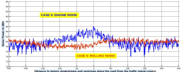
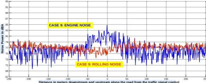
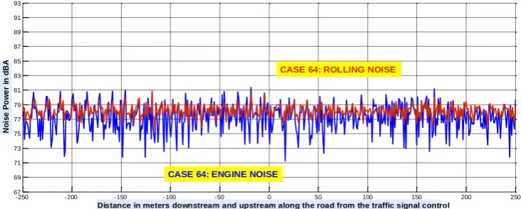
By combining traffic parameters, there were generated 40 cases. From these cases we have chosen the most relevant ones in order to establish some general rules. The set of figures presented below shows the noise power emissions due to traffic along the main road (250 meters upstream and downstream the traffic signal control situated in the junction). The rolling noise is represented by the red color and the engine noise in blue.
Although we have analyzed the influence on noise of certain traffic parameters as: Type of flow: random vs. platoons
Length of the cycles Traffic demand Behavior of the cars
[image:5.595.125.494.550.697.2]In this paper we focus on the influence of prioritization of busses respect to the regular fixed time program of the traffic signals. The analysis of all the cases show a pattern. This pattern is presented below through the comparisons of the cases 6 and 46, 9 and 49: Free flow graphics are also introduced in order to illustrate the influence of the different signaled junctions.
Figure 1 –Case 6: BSP programmed in VAP, random traffic. Cycle: 60 s. Main road demand: 1900 veh/h., from which 120 are buses.
-250 -200 -150 -100 -50 0 50 100 150 200 250 70 72 74 76 78 80 82 84 86 88 90 92 94 96
Distance in meters downstream and upstream along the road from the traffic signal control
N o is e P o w e r in d B A
CASE 6: ENGINE NOISE
Figure 2 –Case 46: The traffic simulation parameters are exactly the same as case 6, except that this time is a fixed time program.
Figure 3 –Case 62: Graphical representation of the noise power level of free traffic flow, keeping the same parameters as in the cases: 6 and 46.
Figure 4 –Case 9: BSP programmed in VAP, random traffic. Cycle: 120 s. Main road demand: 950 veh/h., from which 120 are buses.
-250 -200 -150 -100 -50 0 50 100 150 200 250 70 72 74 76 78 80 82 84 86 88 90 92 94 96
Distance in meters downstream and upstream along the road from the traffic signal control
N o is e P o w e r in d B A
CASE 46: ENGINE NOISE
CASE 46: ROLLING NOISE
-250 -200 -150 -100 -50 0 50 100 150 200 250 70 72 74 76 78 80 82 84 86 88 90 92 94 96
Distance in meters downstream and upstream along the road from the traffic signal control
N o is e P o w e r in d B A
CASE 62: ENGINE NOISE
CASE 62: ROLLING NOISE
-250 -200 -150 -100 -50 0 50 100 150 200 250 67 69 71 73 75 77 79 81 83 85 87 89 91 93
Distance in meters downstream and upstream along the road from the traffic signal control
N o is e P o w e r in d B
A CASE 9: ENGINE NOISE
[image:6.595.127.490.511.657.2]Figure 5 –Case 49: The traffic simulation parameters are exactly the same as case 9, except that this time is a fixed time program
Figure 6 –Case 64: Graphical representation of the noise power level of free traffic flow, keeping the same parameters as in the cases: 9 and 49.
What we can observe in the analysis of all simulations with BSP and Fixed Time is that in a general manner the noise in the proximity of the traffic light is always higher in the FIXED TIME cases. This can be checked in the presented graphics (1 to 4). In these cases the engine noise power is the average during all the simulation time (This includes all the stages of the traffic lights). This means that in these graphics aren`t represented just the most important noise events which take place during stop and go behavior.
More buses more noise problems in Fixed traffic lights. This is not applicable to the BSP cases.
CONCLUSIONS
Regarding the type of flow: (random vs. platoons). It can be observed that the noise upstream is less when the traffic flow is in platoons
Regarding the length of traffic light cycles. It can be observed when the cycles are larger, the noise power increased upstream traffic signal control. This statement is true for fixed traffic regulation and BSP.
Regarding density of the flow. When the level of service is lower (but without reaching traffic jam) the noise is relatively lower (of course, taking into account the density) when compare with lower traffic demand.
Regarding BSP logic. BSP solves the problem of noise, promotes the public transport, without causing any type of negative secondary effects on the mobility of the private traffic.
-250 -200 -150 -100 -50 0 50 100 150 200 250 67
69 71 73 75 77 79 81 83 85 87 89 91 93
Distance in meters downstream and upstream along the road from the traffic signal control
N
o
is
e
P
o
w
e
r
in
d
B
A
CASE 49: ENGINE NOISE
CASE 49: ROLLING NOISE
-250 -200 -150 -100 -50 0 50 100 150 200 250 67
69 71 73 75 77 79 81 83 85 87 89 91 93
Distance in meters downstream and upstream along the road from the traffic signal control
N
o
is
e
P
o
w
e
r
in
d
B
A
CASE 64: ROLLING NOISE
[image:7.595.127.493.317.464.2]REFERENCES
1. A Congestion-Free Bus Network, International Association of Public Transport, December 2001 -
http://www.uitp.org/sites/default/files/cck-focus-papers-files/01%20A%20CONGESTION-FREE%20BUS%20NETWORK.pdf
2. Ashish Bhaskar, Edward Chung, Olivier de Mouzon André-Gilles Dumont, Methodology for Travel Time Estimation on a Signalised Arterial, Young Researchers Seminar, 2007.
3. Report 11/2013. A closer look at urban transport. TERM 2013: transport indicators tracking progress towards environmental targets in Europe, [EEA] European Environment Agency http://www.eea.europa.eu/EEA http://www.eea.europa.eu/, 2013;
4. SILENCE Effectiveness and Benefits of Traffic Flow Measures on Noise Control, European Commission Dg Research Sixth Framework Programme Priority 6 Sustainable Development, Global Change & Ecosystems Integrated Project – Contract N. 516288
5. Margaret Bell, Environmental factors in intelligent transport systems, IEE PROCEEDINGS - INTELLIGENT TRANSPORT SYSTEMS · JULY 2006
6. José Luis Cueto Ancela; Ricardo Hernández Molina, Francisco Fernández Zacarías, Intersecciones semaforizadas en la ciudad y ruido ambiental, TecniAcustica, Valladolid, 2013
7. Prioritisation of public transport in cities, CIVITAS
8. Harriet R. Smith, Brendon Hemily, Miomir Ivanovic, Gannett Fleming, Transit Signal Priority TSP A Planning and Implementation Handbook
9. Prioritisation of public transport in cities, CIVITAS
10. Bert De Coensel, Dick Botteldooren, Filip Vanhove, Steven Logghe, Microsimulation Based Corrections on the Road Traffic Noise Emission Near Intersections, Acta Acustica United with Acustica Vol. 93 (2007) 241 – 252;
11. Bert De Coensel and Dick Botteldooren, Traffic signal coordination: a measure to reduce the environmental impact of urban road traffic?, inter-noise 2011, Osaka japan September, 4-7;
12. Bert De Coensel, A.L. Brown, Deanna Tomerini, Dick Botteldooren, Modeling road traffic noise using distributions for vehicle sound power level, inter-noise 2012, august 19-22, new York;
13. B. De Coensel, A. Can, B. Degraeuwe, I. De Vlieger, D. Botteldooren, Effects of traffic signal coordination on noise and air pollutant emissions, Environmental Modelling & Software 2012, 1-10; 14. E. Chevallier, A. Can, M. Nadji, L. Leclercq, Improving noise assessment at intersections by modeling traffic dynamics, Université de Lyon
ENTPE / INRETS - Laboratoire d’Ingénierie Circulation Transport;
15. Paul Stuart Goodman, B.Eng.(Hons), The Prediction of Road Traffic Noise in Urban Areas, 2001; 16. Serge P. Hoogendoorn, Piet H.L. Bovy, State-of-the-art of Vehicular Traffic Flow Modelling, , Special Issue on Road Traffic Modelling and Control of the Journal of Systems and Control Engineering; 17. Erin Ferguson N. Nezamuddin, ManWo Ng, S. Travis Waller, Guidance for feasibility analysis of candidate sites: handbook, TxDOT Project 0-5913: Feasibility of Speed Harmonization and Peak Period Shoulder Use to Manage Urban Freeway Congestion SEPTEMBER 30, 2009;
18. Emmanuel Bert, Dr Edward Chung, Prof. A.-G. Dumont, Conference paper STRC 2007. 7th Swiss Transport Research Conference. Dynamic Origin-Destination Matrices Estimation Method for urban networks;
19. Managed Lanes-traffic modeling/ Steven Venglas, David Fenno, Samir Goel, Paul Schrader, Operating freeways with Managed Lanes
20. Martin Fellendorf and Peter Vortisch, Chapter 2, Microscopic Traffic Flow Simulator VISSIM pg. 1 21. Antonios Chaziris, Development of a new pro-active vehicle actuated signal control strategy - Evaluation on an urban intersection in Athens, University of Twente, master thesis, 11 April 2011
22. VISSIM Vehicle Actuated Programming (VAP) tutorial, 2006