Lectura Complementaria Rational Expectations and the Theory of Price Movements MUTH

Author(s): John F. Muth

Source: Econometrica, Vol. 29, No. 3 (Jul., 1961), pp. 315-335 Published by: The Econometric Society

Stable URL: http://www.jstor.org/stable/1909635 Accessed: 19/09/2008 06:53

Your use of the JSTOR archive indicates your acceptance of JSTOR's Terms and Conditions of Use, available at

http://www.jstor.org/page/info/about/policies/terms.jsp. JSTOR's Terms and Conditions of Use provides, in part, that unless you have obtained prior permission, you may not download an entire issue of a journal or multiple copies of articles, and you may use content in the JSTOR archive only for your personal, non-commercial use.

Please contact the publisher regarding any further use of this work. Publisher contact information may be obtained at

http://www.jstor.org/action/showPublisher?publisherCode=econosoc.

Each copy of any part of a JSTOR transmission must contain the same copyright notice that appears on the screen or printed page of such transmission.

JSTOR is a not-for-profit organization founded in 1995 to build trusted digital archives for scholarship. We work with the scholarly community to preserve their work and the materials they rely upon, and to build a common research platform that promotes the discovery and use of these resources. For more information about JSTOR, please contact support@jstor.org.

The Econometric Society is collaborating with JSTOR to digitize, preserve and extend access to Econometrica.

RATIONAL EXPECTATIONS AND THE THEORY OF PRICE

MOVEMENTS1

BY JOHN F. MUTH

In order to explain fairly simply how expectations are formed, we advance the hypothesis that they are essentially the same as the predictions of the relevant economic theory. In particular, the hypothesis asserts that the economy generally does not waste information, and that expectations depend specifically on the structure of the entire system. Methods of analysis, which are appropriate under special conditions, are described in the context of an isolated market with a fixed production lag. The interpretative value of the hypothesis is illustrated by introducing commodity speculation into the system.

1. INTRODUCTION

THAT EXPECTATIONS of economic variables may be subject to error has,

for some time, been recognized as an important part of most explanations of changes in the level of business activity. The "ex ante" analysis of the Stockholm School-although it has created its fair share of confusion-is a highly suggestive approach to short-run problems. It has undoubtedly been a major motivation for studies of business expectations and intentions data. As a systematic theory of fluctuations in markets or in the economy, the approach is limited, however, because it does not include an explanation of the way expectations are formed. To make dynamic economic models complete, various expectations formulas have been used. There is, however, little evidence to suggest that the presumed relations bear a resemblance to the way the economy works.2

What kind of information is used and how it is put together to frame an estimate of future conditions is important to understand because the character of dynamic processes is typically very sensitive to the way ex- pectations are influenced by the actual course of events. Furthermore, it is often necessary to make sensible predictions about the way expectations would change when either the amount of available information or the struc-

1 _{Research undertaken for the project, Planning and Control of Industrial Operations,}

under contract with the Office of Naval Research. Contract N-onr-760-(01), Project NR 04701 1. Reproduction of this paper in whole or in part is permitted for any purpose of the United States Government.

An earlier version of this paper was presented at the Winter Meeting of the Eco- nometric Society, Washington, D.C., December 30, 1959.

I am indebted to Z. Griliches, A. G. Hart, M. H. Miller, F. Modigliani, M. Nerlove, and H. White for their comments.

2 _{This comment also applies to dynamic theories in which expectations do not}

ture of the system is changed. (This point is similar to the reason we are curious about demand functions, consumption functions, and the like, instead of only the reduced form "predictors" in a simultaneous equation system.) The area is important from a statistical standpoint as well, because parameter estimates are likely to be seriously biased towards zero if the wrong variable is used as the expectation.

The objective of this paper is to outline a theory of expectations and to show that the implications are-as a first approximation-consistent with the relevant data.

2. THE "RATIONAL EXPECTATIONS" HYPOTHESIS

Two major conclusions from studies of expectations data are the following: 1. Averages of expectations in an industry are more accurate than naive models and as accurate as elaborate equation systems, although there are considerable cross-sectional differences of opinion.

2. Reported expectations generally underestimate the extent of changes that actually take place.

In order to explain these phenomena, I should like to suggest that expectations, since they are informed predictions of future events, are essentially the same as the predictions of the relevant economic theory.3 At the risk of confusing this purely descriptive hypothesis with a pronounce- ment as to what firms ought to do, we call such expectations "rational." It is sometimes argued that the assumption of rationality in economics leads to theories inconsistent with, or inadequate to explain, observed phenomena, especially changes over time (e.g., Simon [29]). Our hypothesis is based on exactly the opposite point of view: that dynamic economic

models do not assume enough rationality.

The hypothesis can be rephrased a little more precisely as follows: that expectations of firms (or, more generally, the subjective probability distribution of outcomes) tend to be distributed, for the same information set, about the prediction of the theory (or the "objective" probability distributions of outcomes).

The hypothesis asserts three things: (1) Information is scarce, and the economic system generally does not waste it. (2) The way expectations are formed depends specifically on the structure of the relevant system describing the economy. (3) A "public prediction," in the sense of Grunberg and Modi- gliani [14], will have no substantial effect on the operation of the economic system (unless it is based on inside information). This is not quite the same thing as stating that the marginal revenue product of economics is zero,

because expectations of a single firm may still be subject to greater error than the theory.

It does not assert that the scratch work of entrepreneurs resembles the system of equations in any way; nor does it state that predictions of en- trepreneurs are perfect or that their expectations are all the same.

For purposes of analysis, we shall use a specialized form of the hypothesis. In particular, we assume:

1. The random disturbances are normally distributed.

2. Certainty equivalents exist for the variables to be predicted.

3. The equations of the system, including the expectations formulas, are linear.

These assumptions are not quite so strong as may appear at first because any one of them virtually implies the other two.4

3. PRICE FLUCTUATIONS IN AN ISOLATED MARKET

We can best explain what the hypothesis is all about by starting the analysis in a rather simple setting: short-period price variations in an isolated market with a fixed production lag of a commodity which cannot be stored.5 The market equations take the form

Ct -AfiPt (Demand),

(3.

Pt Ct (Market equilibrium),

where: Pt represents the number of units produced in a period lasting as long as the production lag,

Ct is the amount consumed,

Pt is the market price in the tth period,

pe is the market price expected to prevail during the tth period on the basis of information available through the (t -1)'st period,

ut is an error term-representing, say, variations in yields due to weather. All the variables used are deviations from equilibrisui3 values.

4 As long as the variates have a finite variance, a linear regression function exists if and only if the variates are normally distributed. (See Allen [2] and Ferguson [12].) The certainty-equivalence property follows from the linearity of the derivative of the appropriate quadratic profit or utility function. (See Simon [28] and Theil [32].)

5 It is possible to allow both short- and long-run supply relations on the basis of

The quantity variables may be eliminated from (3.1) to give

(3.2) Pt== - _-et

The error term is unknown at the time the production decisions are made,

but it is known-and relevant-at the time the commodity is purchased in

the market.

The prediction of the model is found by replacing the error term by its expected value, conditional on past events. If the errors have no serial correlation and Eut = 0. we obtain

(3.3) Ept AfptA

If the prediction of the theory were substantially better than the ex- pectations of the firms, then there would be opportunities for the "insider"

to profit from the knowledge-by inventory speculation if possible, by

operating a firm, or by selling a price forecasting service to the firms. The profit opportunities would no longer exist if the aggregate expectation of the firms is the same as the prediction of the theory:

(3.4) EPt=Pt .

Referring to (3.3) we see that if y//3 - 1 the rationality assumption (3.4)

implies that =0, or that the expected price equals the equilibrium price.

As long as the disturbances occur only in the supply function, price and quantity movements from one period to the next would be entirely along the demand curve.

The problem we have been discussing so far is of little empirical interest, because the shocks were assumed to be completely unpredictable. For most markets it is desirable to allow for income effects in demand and alternative costs in supply, with the assumption that part of the shock variable may be predicted on the basis of prior information. By retracing our steps from (3.2), we see that the expected price would be

(3.5) Pt e Eut .

If the shock is observable, then the conditional expected value or its regression estimate may be found directly. If the shock is not observable, it must be estimated from the past history of variables that can be measured.

Expectations zwith Serially Correlated Distuyrbances. We shall write the u's

distributed random variables 8t with zero mean and variance a2:

(3.6) co~0 r2 _{if ij}

(3.6) 6t =z Wi -Et-i, E8j = 0, E8j =

(o

Any desired correlogram in the u's may be obtained by an appropriate choice of the weights wi.

The price will be a linear function of the same independent disturbances; thus

00

(3.7) it- E wiet-iE

i=0

The expected price given only information through the (t -1)'st period

has the same form as that in (3.7), with the exception that 8t is replaced by

its expected value (which is zero). We therefore have

(3.800 pe O8

O0

(3.8)

i=l1=

If, in general, we let Pt,L be the price expected in period t +L on the

basis of information available through the tth period, the formula becomes

00 (3.9) fit-L,L -E Wist-iE

i=L

Substituting for the price and the expected price into (3.1), which reflect the market equilibrium conditions, we obtain

(3. 10) Wo E-t + 1 + )zwi Et-{ = - zSfet-z .

A i=1 i{=0

Equation (3.10) is an identity in the e's; that is, it must hold whatever

values of ej happen to occur. Therefore, the coefficients of the correspond-

ing ej in the equation must be equal.

The weights Wi are therefore the following:

(3.1 la) p ze ,

(3.1 I1b) Wi -+w (i =1,2,3, *)..

Equations (3.1 1) give the parameters of the relation between prices and price expectations functions in terms of the past history of independent shocks. The problem remains of writing the results in terms of the history of observable variables. We wish to find a relation of the form

00

We solve for the weights V1 in terms of the weights Wj in the following manner. Substituting from (3.7) and (3.8), we obtain

00 00 00 00 t

(3.13) WiVt- EV IWiet-i-i = V Wi 8t-ti.

{=1 ?~=1 i=0 J5 =1

Since the equality must hold for all shocks, the coefficients must satisfy the equations

(3.14) Wi VWiy (i = 1,2,3,...).

1=1

This is a system of equations with a triangular structure, so that it may be solved successively for the coefficients V1, V2, V3,....

If the disturbances are independently distributed, as we assumed before, then wO -1 /8 and all the others are zero. Equations (3.14) therefore imply

(3.15a) t

(3.15b) Pt = _{P+Wost - lete}

These are the results obtained before.

Suppose, at the other extreme, that an exogenous shock affects all future conditions of supply, instead of only the one period. This assumption would be appropriate if it represented how far technological change differed from its trend. Because ut _{is the sum of all the past ej, wi} 1 (i = 0,1,2,...). From (3.1 1),

(3.16a) Wo -1/fl,

(3.16b) Wi l/0 +y)

From (3.14) it can be seen that the expected price is a geometrically weighted moving average of past prices:

(3.17) ( _y

)

.

pt y _P t: _{+ yJt-}

Deviations from Rationality. Certain imperfections and biases in the expectations may also be analyzed with the methods of this paper. Allowing for cross-sectional differences in expectations is a simple matter, because their aggregate effect is negligible as long as the deviation from the rational forecast for an individual firm is not strongly correlated with those of the others. Modifications are necessary only if the correlation of the errors is large and depends systematically on other explanatory variables. We shall examine the effect of over-discounting current information and of differences in the information possessed by various firms in the industry. Whether such biases in expectations are empirically important remains to be seen. I wish only to emphasize that the methods are flexible enough to handle them.

Let us consider first what happens when expectations consistently over- or under-discount the effect of current events. Equation (3.8), which gives the optimal price expectation, will then be replaced by

00

(3.18) Pt = fi Wiet-i + I Wi Et-i

i=2

In other words the weight attached to the most recent exogenous dis- turbance is multiplied by the factor

f1,

If we use (3.18) for the expected price instead of (3.8) to explain market price movements, then (3.1 1) is replaced by

(3.19a) Wo wo

(3.19b) WW WI

(3.19c) Wi Wi (i = 2,3,4,...).

/3+y

The effect of the biased expectations on price movements depends on the statistical properties of the exogenous disturbances.

If the disturbances are independent (that is, wo =1 and wj = 0 for i > 1), the biased expectations have no effect. The reason is that successive obser- vations provide no information about future fluctuations.

On the other hand, if all the disturbances are of a permanent type (that

is, w0 = _w, = ... = 1), the properties of the expectations function are

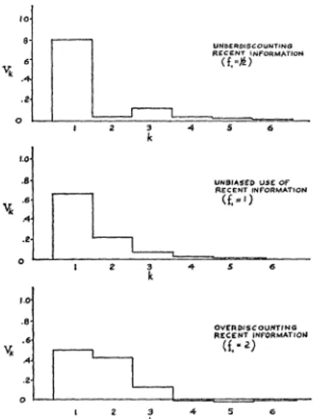
significantly affected. To illustrate the magnitude of the differences, the parameters of the function

00

are compared in Figure 3.1 for ,B 2y and various values of fi. If current

information is under-discounted (f= 1/2), the weight VI attached to the

latest observed price is very high. With over-discounting (fi 2), the

weight for the first period is relatively low.

UNDERDI COUNTING

Vk .4, ~~~~~~~RECENT INFORMATION

a 2 3 4 5 6

k

.8 ~~~~~~~~UN31A5ED USE oF RECENT INFORMATION Uk *

Io i i 2 4 5 1

OVERD SCOUNTINGC

, ~~~~~~~~RECENT INFORMATIOW

1 2 3 4 5 6

FIGURE 3.1.-Autoregression Coefficients of Expectations for Biased Use of Recent

Information. (wo = w, = ... == 1).

The model above can be interpreted in another way. Suppose that some of the firms have access to later information than the others. That is, there is a lag of one period for some firms, which therefore form price expectations according to (3.8). The others, with a lag of two periods, can only use the following:

, 00

(3.20) pt t-= Ew

i=2

Then the aggregate price expectations relation is the same as (3.18), if fi represents the fraction of the firms having a lag of only one period in obtain- ing market information (that is, the fraction of "insiders").

4. EFFECTS OF INVENTORY SPECULATION

price expectation with independent disturbances in the supply function then turns out to have the form

(4.1) ft'At_i

where the parameter A would be somewhere between zero and one, its value depending on the demand, supply, and inventory demand parameters.

Speculation with moderately well-informed price expectations reduces the variance of prices by spreading the effect of a market disturbance over several time periods, thereby allowing shocks partially to cancel one another out. Speculation is profitable, although no speculative opportunities remain. These propositions might appear obvious. Nevertheless, contrary views have been expressed in the literature.6

Before introducing inventories into the market conditions, we shall briefly examine the nature of speculative demand for a commodity.

Optimal Speculation. We shall assume for the time being that storage, interest, and transactions costs are negligible. An individual has an opportun- ity to purchase at a known price in the tth period for sale in the succeeding period. The future price is, however, unknown. If we let It represent the speculative inventory at the end of the tth period,7 then the profit to be

realized is

(4.2) at-It(pt+1-Pt).

Of course, the profit is unknown at the time the commitment is to be made. There is, however, the expectation of gain.

The individual demand for speculative inventories would presumably be based on reasoning of the following sort. The size of the commitment depends on the expectation of the utility of the profit. For a sufficiently small range of variation in profits, we can approximate the utility function by the first few terms of its Taylor's series expansion about the origin:

(4.3) Ut - 0 (t) _{(O) +} ?' _{(O) at +"2 O)' (t} +...

The expected utility depends on the moments of the probability distribu-

tion of a:

(4.4) Eut - (0) + 0'(O) Ent + 0) Eat

6 _{See Baumol [5]. His conclusions depend on a nonspeculative demand such that}

prices would be a pure sine function, which may always be forecast perfectly.

From (4.2) the first two moments may be found to be

(4.5a) Ent = _{It(Pt?i-fPt),}

(4.5b) E7ct= Ia[t2,i +(Pi-Pt)2],

where

pt+l

(4.6) Eut = 0 (0) + 0' (0) It (Pt+i -Pt) + 2 q" (0) i2[U2,i + (Pt+i-Pt) 2] +e _..

The inventory therefore satisfies the condition

47)dEu

(4.7)

~

The inventory position would, to a first approximation, be given by

(4.8) It (0 (pt+1-

q (0) [c,l + (P 2i- Pt)2]

If 0' (0) > 0 and 0q" (0) < 0, the above expression is an increasing function

of the expected change in prices (as long as it is moderate).

At this point we make two additional assumptions: (1) the conditional variance, at1, is independent of

Pe,

(4.9) It = x _{(Pt+' -Pt),}

where = (0)at,= (0)/0" 1

Note that the coefficient ax depends on the commodity in only one way: the variance of price forecasts. The aggregate demand would, in addition, depend on who holds the stocks as well as the size of the market. For some commodities, inventories are most easily held by the firms.9 If an organized futures exchange exists for the commodity, a different population would

8 This form of the demand for speculative inventories resembles that of Telser [31] and Kaldor [20].

be involved. In a few instances (in particular, durable goods), inventory accumulation on the part of households may be important.

The original assumptions may be relaxed, without affecting the results significantly, by introducing storage or interest costs. Margin requirements may, as well, limit the long or short position of an individual. Although such requirements may primarily limit cross-sectional differences in positions, they may also constrain the aggregate inventory. In this case, we might reasonably expect the aggregate demand function to be nonlinear with an upper "saturation" level for inventories. (A lower level would appear for aggregate inventories approaching zero.)

Because of its simplicity, however, we shall use (4.9) to represent inven- tory demand.

Market Adjustments. We are now in a position to modify the model of Section 3 to take account of inventory variations. The ingredients are the supply and demand equations used earlier, together with the inventory equation. We repeat the equations below (Pt represents production and Ct consumption during the tth period:

(4. 1 Oa) Ct -f.Pt (Demand) ,

(4. 1Ob) Pt yPe +Ut (Supply),

(4.1 Oc) It o=(Pt+i -Pt) (Inventory speculation)

The market equilibrium conditions are

(4.11) Ct +It=Pt +It-1.

Substituting (4. 10) into (4.1 1), the equilibrium can be expressed in terms of prices, price expectations, and the disturbance, thus

(4.12) -(o +f)ft +oNpt+i - (oa +y)PA- opt-i +Ut-.

The conditions above may be used to find the weights of the regression functions for prices and price expectations in the same way as before. Substituting from (3.6), (3.7), and (3.8) into (4.12), we obtain

00 00

( +) I Wi st-i +a I Wi,6t+l-i

(4. 13) i=? i=1

00 00 ₀₀

- _{(X +'y) z Wist- -a E Wf t-1-i +} E fWt-i -

-=0 i=0

equations must be satisfied:10

(4.14a) -(oN

+13)

(4.14b) ;Wi-_ (2cN + p +y) Wi + NWj+j = w (i - 1,2,3,..) . Provided it exists, the solution of the homogeneous system would be of the form

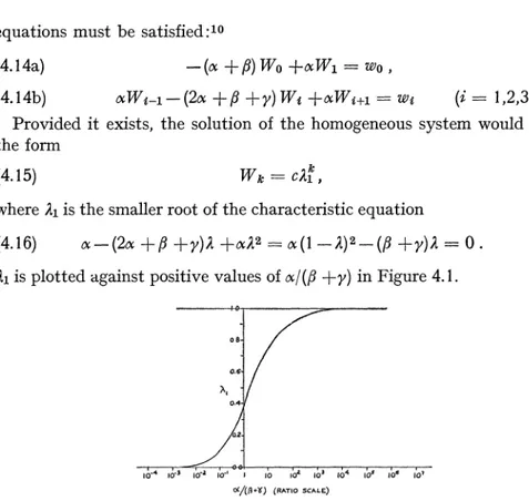
(4.15) Wk = C21

where 21 is the smaller root of the characteristic equation

(4.16)

_{N-(2N +#}

A1 is plotted against positive values of cx/(f +y) in Figure 4.1.

0.6

0 .

*, 3- lol? l 17 3 104 16f 1o6 l 0(/(0+d) (RATIO SCALE)

FIGURE 4.1.-Characteristic Root as a Function of c/(f+y).

A unique, real, and bounded solution to (4.14) will exist if the roots of the characteristic equation are real. The roots occur in reciprocal pairs, so that if they are real and distinct exactly one will have an absolute value less than unity. For a bounded solution the coefficient of the larger root vanishes; the initial condition is then fitted to the coefficient of the smaller root.

The response of the price and quantity variables will be dynamically stable, therefore, if the roots of the characteristic equation are real. It is easy to see that they will be real if the following inequalities are satisfied:

(4.17a) >0)

(4.17b) ,B+y > O.

The first condition requires that speculators act in the expectation of gain (rather than loss). The second is the condition for Walrasian stability. Hence an assumption about dynamic stability implies rather little about

10 _{The same system appears in various contexts with embarrassing frequency. See}

the demand and supply coefficients. It should be observed that (4.17) are not necessary conditions for stability. The system will also be stable if both inequalities in (4.17) are reversed (!) or if 0 > x/(Q +y) > - 1/4. If N = 0, there is no "linkage" from one period of time to another, so the system is dynamically stable for all values of : + y.

Suppose, partly by way of illustration, that the exogenous disturbances affecting the market are independently distributed. Then we can let wo I I and wzc 0 (i > 1). The complementary function will therefore be the complete solution to the resulting difference equation. By substituting (4.15) into (4.14a), we evaluate the constant and find

(4.18) Wk - 1

) -N2e Al

The weights Ve may be found either from (3.14) or by noting that the resulting stochastic process is Markovian. At any rate, the weights are

(4.19) _Vk

{21,

The expected price is therefore correlated with the previous price, and the rest of the price history conveys no extra irnformation, i.e.,

(4.20) pt ipt-_

where the parameter depends on the coefficients of demand, supply, and inventory speculation according to (4.16) and is between 0 and 1. If inven- tories are an important factor in short-run price determination, 21 will be very nearly unity so that the time series of prices has a high positive serial correlation.11 If inventories are a negligible factor, 21 is close to zero and leads to the results of Section 3.

Effects of Inventory Specuqlation. Substituting the expected price, from (4.20), into (4.10), we obtain the following system to describe the operation of the market:

(4.21 a) Ct -Pt

(4.2 1b) Pt =y2AlPt- + Et.

(4.21c) It --x(l-2l)P = tv

The market conditions can be expressed in terms of supply and demand by including the inventory carryover with production and inventory carry-

11 _{If the production and consumption flows are negligible comparedwiththe spec-}

TABLE 4.1

EFFECTS OF INVENTORY SPECULATION

Description Symbol General Approximation

Formula for Small x

1. Characteristic root _Al [eq. (4.16)1 C/(fl + Y)

2. Standard deviation WOp W I(l _A2)-1/2a a

of prices

3. Standard deviation e r)

of expected price _aP + Y)

4. Standard deviation (2 _2I2a2)1/ r _my~ 1

of output ap ( + /2 + _{2fl(fl+ y)]}

5. Mean producers' EPt pt y2 +w 2 _a2

revenue E P

6. Mean speculators' EIt(Pt+i-Pt) c(1- 2i) _Ma2

revenue

2 2

7. Mean consumers' _{ECtpt -} 2 -- __)a2

expenditure p p

Notes: (1) a is the standard deviation of the disturbance in the supply function (4.10b) with wo = 1 and wi = W2 = ... =0 .

(2) Wo = - /[j,9?(l -ki)].

forward with consumption; thus,

(4.22) Qt Ct +It (Demand),

Qt Pt + It-i (Supply).

Substituting from (4.21) we obtain the system:

(4.23a) Qt =

-[I

(4.23b) Qt = [y21-L ( -21)lPt-i +?t (Supply)

The coefficient in the supply equation is reduced while that of the demand equation is increased. The conclusions are not essentially different from those of Hooton [18]. The change is always enough to make the dynamic response stable.

If price expectations are in fact rational, we can make some statements about the economic effects of commodity speculation. (The relevant formulas are summarized in Table 4.1.) Speculation reduces the variance of prices by spreading the effect of a disturbance over several time periods. From Figure 4.2, however, we see that the effect is negligible if LX is much less than the sum of P and y. The standard deviation of expected prices first increases

decreases because of the small variability of actual prices. The variability of factor inputs and production follows roughly the same pattern (cf. Kaldor [20]).

PRICES

.4\

EXPECTED PRICES

10'4 1-3 to-a2 o-o I iO io 103 104 IOc le jo7 -zj (RAu-r sCALE)

FIGURE 4.2.-Standard Deviation of Prices and Expected Prices as a Function of cl(f + y) for B = _y.

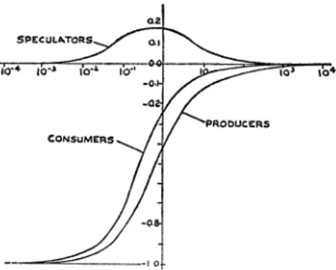
In Figure 4.3 we see that mean income to speculators is always positive and has a maximum value slightly to the left of that for expected prices. Producers' revenue and consumers' expenditures both increase with oc. Consumers' expenditures increase at first a little faster than the revenue of the producers. The effect of speculation on welfare is therefore not obvious.

Q2 SPECULAToTORS

//POODUCER5 CONSUMERS .

FIGURE 4.3.-Mean Income of Producers and Speculators, and Mean Expenditures of Consumers as a Function of cl/(fl + y) for fi = y.

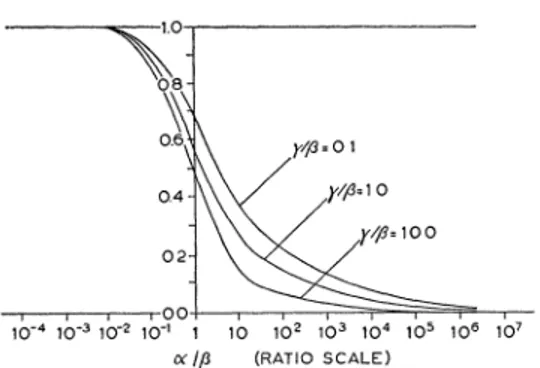
The variability of prices for various values of

y/fl

of _N/lP in Figure 4.4. The general shape of the curve is not affected by values

-108

0X X =

0Ol 0.4

-

I 0 - 1 0

02-

I I00

10o4 10-3 10-2 10-1 1 10 102 103 104 105 10i 107 aX /, (RATIO SCALE)

FIGURE 4.4-Standard Deviation of Prices for Various Values of y/f as a Function

of o0/#.

5. RATIONALITY AND COBWEB THEOREMS

It is rather surprising that expectations have not previously been regarded as rational dynamic models, since rationality is assumed in all other aspects of entrepreneurial behavior. From a purely theoretical standpoint, there are good reasons for assuming rationality. First, it is a principle applicable to all dynamic problems (if true). Expectations in different markets and systems would not have to be treated in completely different ways. Second, if ex- pectations were not moderately rational there would be opportunities for economists to make profits in commodity speculation, running a firm, or selling the information to present owners. Third, rationality is an assump- tion that can be modified. Systematic biases, incomplete or incorrect infor- mation, poor memory, etc., can be examined with analytical methods based on rationality.

Imfplications of Cobweb Theorems. If the market equilibrium conditions of (3.1) are subjected to independent shocks in the supply function, the prediction of the theory would be

(5.1) E(Pt IPt-1,Pt-2,...)

As a result, the prediction of the cobweb theory would ordinarily have the sign opposite to that of the firms. This, of course, has been known for a long time. Schultz noted that the hypothesis implies farmers do not learn from experience, but added: "Such a behavior is not to be ruled out as extremely improbable" [27, p. 78].

The various theories differ primarily in what is assumed about price expectations. The early contributors (through Ezekiel [11]) have assumed that the expected price is equal to the latest known price. That is,

(5.2) Pt-Pt1.

Goodwin [13] proposed the extrapolation formula,

(5.i3) pte = pt-1l- LO.(pt-1 -,t-2) fi

That is, a certain fraction of the latest change is added on to the latest observed price. Depending on the sign of e, which should be between -1 and + 1, we can get a greater variety of behavior. It is still the case, however, that farmers' expectations and the prediction of the model have the opposite

sign.

A third expectations formula is much more recent. The adaptive expec- tations model, used by Nerlove [25], satisfies the following equation:

(5.4) pt = t-l +(tl t-l)f

The forecast is changed by an amount proportional to the most recently observed forecast error. The solution of the difference equation gives the price expectation as a geometrically weighted moving average:

00

(5.5) ep

J=O

two kinds of models according to the properties of firms' expectations and the cyclical characteristics of commodity prices and output.

Expectations of Firms. There is some direct evidence concerning the quality of expectations of firms. Heady and Kaldor [16] have shown that, for the period studied, average expectations were considerably more

TABLE 5.1

PROPERTIES OF COBWEB MODELS

Expectation Prediction Stability pe, E (pt p pt-i,...) Conditions

(A) Classical (Schultz- Y e

Tinbergen-Ricci) Pt-i -Pt y <P

1 1

(B) Extrapolative (I -eQ)Pt- ? ept-2 i Y e _i 1-2Q' 3

(Goodwin) (-1 < < 1) f e 1

00

(C) Adaptive (Nerlove) X1 ( )--pt-; pt y 2-I

(O < q<1) f

(D) Rational 0 0 +?Y ? 0

(E) Rational (with Alpt -1 _xlpt-I > 0

speculation) (O < Al < 1) iPt ? +y > ?

Note: The disturbances are normally and independently distributed with a constant variance.

accurate than simple extrapolation, although there were substantial cross- sectional differences in expectations. Similar conclusions concerning the accuracy have been reached, for quite different expectational data, by Modigliani and Weingartner [23].

If often appears that reported expectations underestimate the extent of changes that actually take place. Several studies have tried to relate the two according to the equation:

(5.6) pt= bp

t

Bossons and Modigliani [6] have pointed out that the size of the estimated

coefficient,

&,

be seen quite clearly as follows. The rational expectations hypothesis states that, in the aggregate, the expected price is an unbiased predictor of the actual price. That is,

(5.7) pt =pt +Vt, EP evt O, Evt O.

The probability limit of the least squares estimate of b in (5.6) would then be given by

(5.8) Plim

6

Cycles. The evidence for the cobweb model lies in the quasi-periodic fluctuations in prices of a number of commodities. The hog cycle is perhaps the best known, but cattle and potatoes have sometimes been cited as others which obey the "theorem." The phase plot of quantity with current and lag- ged price also has the appearance which gives the cobweb cycle its name.

A dynamic system forced by random shocks typically responds, however, with cycles having a fairly stable period. This is true whether or not any characteristic roots are of the oscillatory type. Slutzky [30] and Yule [34] first showed that moving-average processes can lead to very regular cycles. A comparison of empirical cycle periods with the properties of the solution of a system of differential or difference equations can therefore be misleading whenever random shocks are present (Haavelmo [15]).

The length of the cycle under various hypotheses depends on how we measure the empirical cycle period. Two possibilities are: the interval

TABLE 5.2

CYCLICAL PROPERTIES Or COBWEB MODELS

Serial Mean Interval Mean Interval Correlation Between Successive Between Successive Of Prices, ri Upcrosses, L Peaks or Troughs, L'

(A) Classical rl < O

(B) Extrapolative = <e 0 2L ₄ 2 L 3

(C) Adaptive < _r) < O

(D) Rational Iq = O L = 4 L' = 3

(E) Rational - Al > ? L > 4 3 < L' < 4

with storage

Note: The disturbances are assumed to be normally and independently distributed with a constant variance. f and v

between successive "upcrosses" of the time series (i.e., crossing the trend line from below), and the average interval between successive peaks or troughs. Both are given in Table 5.2, which summarizes the serial correlation of prices and mean cycle lengths for the various hypotheses.12

That the observed hog cycles were too long for the cobweb theorem was first observed in 1935 by Coase and Fowler [8, 9]. The graph of cattle prices presented given by Ezekiel [11] as evidence for the cobweb theorem implies an extraordinarily long period of production (five to seven years). The interval between successive peaks for other commodities tends to be longer than three production periods. Comparisons of the cycle lengths should be interpreted cautiously because they do not allow for positive serial correlation of the exogenous disturbances. Nevertheless, they should not be construed as supporting the cobweb theorem.

Carnegie Institute of Technology

REFERENCES

[1] AKERMAN, G.: "The Cobweb Theorem; A Reconsideration," Quarterly Journal of Economics, 71: 151-160 (February, 1957).

[2] ALLEN, H. V.: "A Theorem Concerning the Linearity of Regression," Statistical Research Memoirs, 2: 60-68 (1938).

[3] ARROW, K. J., AND L. HURWICZ: "On the Stability of Competitive Equilibrium I," Econometrica, 26: 522-552 (October, 1958).

[4] ARROW, K. J., H. D. BLOCK, AND L. HURWICZ: "On the Stability of Competitive

Equilibrium II," Econoometrica, 27: 82-109 (January, 1959).

[5] BAUMOL, W. J.: "Speculation, Profitability, and Stability," Review of Econoomics and Statistics, 39: 263-271 (August, 1957).

[6] BossONS, J. D., AND F. MODIGLIANI: "The Regressiveness of Short Run Business Expectations as Reported to Surveys-An Explanation and Its Implications,"

Unpublished, no date.

[7] BUCHANAN, N. S.: "A Reconsideration of the Cobweb Theorem," Journal of Political Econoomy, 47: 67-81 (February, 1939).

[8] COASE, R. H., AND R. F. FOWLER: "The Pig-Cycle in Great Britain: An Explana-

tion," Econoomica, 4 (NS): 55-82 (1937).

[9] : "Bacon Production and the Pig-Cycle in Great Britain," Ecoinomica, 2 (NS): 143-167 (1935). Also "Reply" by R. Cohen and J. D. Barker, pp. 408-422, and "Rejoinder" by Coase and Fowler, pp. 423-428 (1935).

[10] DEAN, G. W., AND E. 0. HEADY: "Changes in Supply Response and Elasticity For Hogs," Journal of Farm Econoomics, 40: 845-860 (November, 1958). [11] EZEKIEL, M.: "The Cobweb Theorem," Quiarterly Journal of Econoomics, 52:

255-280 (February, 1938). Reprinted in Readings in Business Cycle Theory. [12] FERGUSON, T.: "On the Existence of Linear Regression in Linear Structural

Relations," University of California Publications in Statistics, Vol. 2, No. 7, pp. 143-166 (University of California Press, 1955).

12 _{See Kendall [21, Chapters 29 and 30, especially pp. 381 ff.] for the relevant}

[13] GOODWIN, R. M.: "Dynamical Coupling With Especial Reference to Markets Having Production Lags," Econometrica, 15: 181-204 (1947).

[14] GRUNBERG, E., AND F. MODIGLIANI: "The Predictability of Social Events," Journal of Political Economy, 62: 465-478 (December, 1954).

[15] HAAVELMO, T.: "The Inadequacy of Testing Dynamic Theory by Comparing

Theoretical Solutions and Observed Cycles," Econometrica, 8: 312-321 (1940). [16] HEADY, E. O., AND D. R. KALDOR: "Expectations and Errors in Forecasting Agricultural Prices," Journal of Political Economy, 62: 34-47 (February, 1954). [17] HOLT, C. C., F. MODIGLIANI, J. F. MUTH, AND H. A. SIMON: Planning Production,

Inventories, and Work Force (Prentice-Hall, 1960).

[18] HOOTON, F. G.: "Risk and the Cobweb Theorem," Economic Journal, 60: 69-80 (1950).

[19] JESNESS, 0. B.: "Changes in the Agricultural Adjustment Program in the Past 25

Years," Journal of Farm Economics, 40: 255-264 (May, 1958).

[20] KALDOR, N.: "Speculation and Economic Stability," Rev. Economic Studies, 7:

1-27 (1939-1940).

[21] KENDALL, M. G.: The Advanced Theory of Statistics, Vol. II (Hafner, 1951).

[22] : "The Analysis of Economic Time-Series-Part I: Prices," Journal of the Royal Statistical Society, Series A, 16 : 11-34 (1953).

[23] MODIGLIANI, F., AND H. M. WEINGARTNER: "Forecasting Uses of Anticipatory Data on Investment and Sales," Quarterly Journal of Economics, 72: 23-54 (February, 1958).

[24] MUTH, J. F.: "Optimal Properties of Exponentially Weighted Forecasts," Journal of the American Statistical Association 55: 299-306 (June, 1960). [25] NERLOVE, M.: "Adaptive Expectations and Cobweb Phenomena," Quarterly

Journal of Economics, 73: 227-240 (May, 1958).

[26] The Dynamics of Supply: Estimation of Farmers' Response to Price (John

Hopkins Press, 1958).

[27] SCHULTZ, H.: The Theory and Measurement of Demand (University of Chicago

Press, 1958).

[28] SIMON, H. A.: "Dynamic Programming Under Uncertainty with a Quadratic

Criterion Function," Econometrica, 24: 74-81 (1956).

[29] : "Theories of Decision-Making in Economics," American Economic

Review, 49: 223-283 (June, 1959).

[30] SLUTZKY, E.: "The Summation of Random Causes as the Source of Cyclic Pro- cesses," Econometrica, 5: 105-146 (April, 1937).

[31] TELSER, L. G.: "A Theory of Speculation Relating Profitability and Stability," Review of Economics and Statistics, 61: 295-301 (August, 1959).

[32] THEIL, H.: "A Note on Certainty Equivalence in Dynamic Planning," Econome- trica, 25: 346-349 (April, 1957).

[33] : Economic Forecasts and Policy (North-Holland, 1958).