OPEN ACCESS
entropy
ISSN 1099-4300 www.mdpi.com/journal/entropyArticle
Generalized Complexity and Classical-Quantum Transition
A. M. Kowalski1,2, Angelo Plastino2,⋆and Montserrat Casas3
1
Comision de Investigaciones Cientificas (CIC), Argentina
2
La Plata Physics Institute (IFLP), Exact Sciences Fac., National University (UNLP), Argentina’s National Research Council (CCT-CONICET), C.C. 727, (1900) La Plata, Argentina
3
Departament de F´ısica and IFISC, Universitat de les Illes Balears, 07122 Palma de Mallorca, Spain E-mails: [email protected]; [email protected]
⋆ Author to whom correspondence should be addressed. E-mail: [email protected]
Received: 10 January 2009/ Accepted: 26 February 2009 / Published: 4 March 2009
Abstract: We investigate the classical limit of the dynamics of a semiclassical system that represents the interaction between matter and a given field. On using as a quantifier the q -Complexity, we find that it describes appropriately the quantum-classical transition, detecting the most salient details of the changeover. Additionally theq-Complexity results a better quan-tifier of the problem than the q-entropy, in the sense that the q-range is enlarged, describing the q-Complexity, the most important characteristics of the transition for allq-value.
Keywords: Generalized entropy; Semiclassical theories; Quantum chaos; Statistical com-plexity.
PACS:89.70.Cf. 03.65.Sq, 05.45.Mt
1. Introduction
techniques based on symbolic dynamics [7], Fourier analysis [8], and wavelet transform [9] (among oth-ers). The applicability of these approaches depends on the data-characteristics, i.e., stationarity, length of the series, parameter-variations, levels of noise-contamination, etc. The distinct treatments at hand “capture” the global aspects of the dynamics, but they are not equivalent in their ability to discern physi-cal details. However, one should recognize that we are here referring to techniques defined in an ad-hoc fashion, not derived directly from the dynamical properties of the pertinent system themselves.
Statistical complexity. In [3], L´opez-Ruiz, Mancini and Calbet (LMC) advanced a statistical com-plexity measure (SCM) based on the notion of “disequilibrium” as a quantifier of the degree of physical structure in a time series. Given a probability distribution associated with a system’s state, the LMC mea-sure is the product of an normalized entropy H times a distance to the uniform-equilibrium stateQ. It vanishes for a totally random process and for a periodic one. Mart´ın et al. [10] improved on this measure by modifying the distance-component (in the concomitant probability space). In Ref. [10],Qis built-up using Wootters’ statistical distance whileH is a normalized Shannon-entropy. Regrettably enough, the ensuing statistical complexity measure is neither an intensive nor an extensive quantity, although it does yield useful results. A reasonable complexity measure should be able to distinguish among different de-grees of periodicity and it should vanish only for periodicity unity. In order to attain such goals it would seem desirable to give this statistical measure an intensive character. This was achieved in Ref. [4] ob-taining a SCM that is (i) able to grasp essential details of the dynamics, (ii) an intensive quantity, and (iii) capable of discerning among different degrees of periodicity and chaos.
Deformedq-statistics. It is a well-known fact that physical systems that are characterized by either long-range interactions, long-term memories, or multi-fractal nature, are best described by a generalized statistical mechanics’ formalism [11] that was proposed 20 years ago: the so-called q-statistics. More precisely, Tsallis [12] advanced in 1988 the idea of using in a thermodynamics’ scenario an entropic form, the Harvda-Chavrat one, characterized by the entropic index q ∈ R (q = 1 yields the orthodox Shannon measure):
Sq=
1 (q−1)
Ns
X
i=1
[pi−(pi)q], (1)
where pi are the probabilities associated with the associated Ns different system-configurations. The entropic index (or deformation parameter) q describes the deviations of Tsallis entropy from the standard Boltzmann-Gibbs-Shannon-one
S =−
Ns
X
i=1
piln(pi). (2)
It is well-known that the orthodox entropy works best in dealing with systems composed of either inde-pendent subsystems or interacting via short-range forces whose subsystems can access all the available phase space [11]. For systems exhibiting long-range correlations, memory, or fractal properties, Tsallis’ entropy becomes the most appropriate mathematical form [13–16].
authors (see Ref. [19] and references therein).
It is reasonable to relay onq-statistics [36], so as to gather insights into the
quantum − semiclassical − classical transition (CLQM). (3)
Why? Because we know that the classic to quantum route traverses high complexity regions of the appropriate phase space where chaos reigns, interrupted often by quasi-periodic windows [19–21]. In the semiclassical parcel of the associated trajectory one encounters also strong correlation between classical and quantum degrees of freedom [20,21].
In [36] we showed that a wavelet-evaluated q-entropy not only describes correctly the quantum-classical border but also that the associated deformation-parameter q itself characterizes the different regimes involved in the concomitant process, detecting the most salient fine details of the transition. The purpose of the present effort is to gather new insights into theq-statistics’ contribution to this problem by recourse to a new tool: theq−statistical complexity. Since in this work the pertinentq-quantifiers are computed using “wavelet techniques” (whose utility has been evidenced in ([20,21]), we provide a brief wavelet-r´esum´e in the Appendix.
2. A semi-classical model and the CLQM
Quite a bit of quantum insight is to be gained from semiclassical perspectives. Several methodologies are available (WKB, Born-Oppenheimer approach, etc.). Here we consider two interacting systems: a classical and a quantal ones. This can be done whenever the quantum effects of one of the two systems are negligible in comparison to those of the other one. Examples can be readily found. We can just mention Bloch-equations [23], two-level systems interacting with an electromagnetic field within a cav-ity, Jaynes-Cummings semiclassical model [24–27], collective nuclear motion [28], etc. We shall focus attention upon a special bipartite model [29–31] that has been found useful with reference to problems in such diverse fields as chaos, wave-function collapse, measurement processes, and cosmology [32]. In order to investigate theq-statistics’ contribution to the CLQM problem by recourse to theq−statistical complexity (our goal here) we shall consider a trivial generalization of the semi-classical Hamiltonian that represents the zero-th mode contribution of a strong external field to the production of charged meson pairs [30,31]. It reads
ˆ
H = 1
2
µ
ˆ
p2
mq
+ PA 2
mcl
+ mqω
2 ˆ
x2 
, (4)
where i) xˆ and pˆare quantum operators, ii) A and PA classical canonical conjugate variables and iii)
ω2
=ωq2+e2A2is an interaction term that introduces nonlinearity,ωqbeing a frequency. The quantities
mqandmcl are masses, corresponding to the quantum and classical systems, respectively. As shown in Ref. [33], in dealing with (4) one faces an autonomous system of nonlinear coupled equations
dhˆx2i
dt =
hLˆi
mq ,
dhpˆ2i
dt =−mqω
2
hLˆi, dhdtLˆi = 2(hmpˆ2qi −mq ω2hxˆ2i), dA
dt = PA
mcl ,
dPA
dt =−e
2
mqAhxˆ2i, Lˆ = ˆxpˆ+ ˆpxˆ .
(5)
The system of Eqs. (5) follows immediately from Ehrenfest’s relations [33]. To study the classical limit we need to also consider the classical counterpart of the Hamiltonian (4)
H = 1
2
· p2
mq
+ PA 2
mcl
+ mq(ω
2
q +e
2
A2)x2 ¸
where all the variables are classical. Recourse to Hamilton’s equations allows one to find the classical version of Eqs. (5) (see Ref. [33] for details). Let i)E stand for the total energy of the system and ii)I
be an invariant of the motion described by the system (5), related to the Uncertainty Principle, that reads
I = hxˆ2
ihpˆ2
i − hLˆi
2
4 . (7)
It is easy to see that a classical computation of I yieldsI = x2
p2
−L2
/4 ≡ 0. The classical limit is obtained by letting [33] the “relative energy”
Er = |E|
I1/2ω
q
→ ∞. (8)
A measure of the degree of convergence between classical and quantum results in the limit of Eq. (8) is given by the normN of the vector∆u=u−ucl [33]
N∆u =|u−ucl|, (9)
where the three components vector u = (hxˆ2
i,hpˆ2
i,hLˆi) is the “quantum” part of the solution of the system Eqs. (5) and ucl = (x2, p2, L) its classical partner. A detailed study of our present model was performed in Refs. [33, 34]. We summarize here the main results of these references that are pertinent for our discussion. In plotting diverse dynamical quantities versusEr(as it grows from unity to∞), one findsan abrupt change in the system’s dynamics for special values of Er, to be denoted byErcl. From this value onwards, the pertinent dynamics starts converging to the classical one. It is thus possible to assert thatErcl provides us with anindicatorof the presence of a quantum-classical “border”. The zone
Er < Ercl, (10)
corresponds to the semi-quantal regime investigated in Ref. [34]. This regime, in turn, is characterized by two different sub-zones [33]. i) One of them is an almost purely quantal one, in which the micro-scopic quantal oscillator is just slightly perturbed by the classical one, and ii)the other section exhibits a transitional nature (semi-quantal). The border between these two sub-zones can be well characterized by a “signal” valueErP. A significant feature of this point resides in the fact that, forEr ≥ErP,chaos is always found. The relative number of chaotic orbits (with respect to the total number of orbits) grows withEr and tends to unity forEr → ∞[33, 34]. Thus, asEr grows fromEr = 1(the “pure quantum instance”) toEr → ∞(the classical situation), a significant series ofmorphology-changesis detected, specially in the transition-zone (ErP ≤Er ≤Ercl). The concomitant orbits exhibit features that are not easily describable in terms of Eq. (9), which is aglobalmeasure of the degree of convergence in ampli-tude (of the signal). What one needs instead is a statistical type of characterization, as that described in Refs. [20,21,35].
2.1. Previousq-entropy Results
In [36], we found that the normalized Tsallis wavelet entropyHSq, in the range0< q <5, correctly
measure is unable to do, concluding that it is the most appropriate entropy, and not the orthodox, q = 1 of Shannon’s. Additionally, we discovered other transition-detectors in addition to the normalized Tsallis-entropy, specially its curvature when we plot it for that particular q−value, qM, for whichHSq
has a minimum. qM itself turned out to a good transition-indicator. These last results affirm that the deformation parameterqby itself can be regarded as the “looking glass” through which one can observe the quantum-classical transition. We are ready now to start presenting the new results of this contribution: the role played by theq-complexity in describing the route from the quantum regime to the classical one.
3. Present results
3.1. Introducing theq-statistical complexity
The Statistical Complexity can be viewed as a functional C[P] that characterizes the probability distributionP associated to the time series generated by the dynamical system under study. It quantifies not only randomness but also the presence of correlational structures [3, 4, 10]. This quantity is of the form [22]
C[P] =Q[P, Pe] HS[P], (11)
where, to the probability distribution P, we associate the entropic measureHS[P] = S[P]/Smax, with
Smax = S[Pe] (0 ≤ HS ≤ 1). Pe is the uniform distribution and S is an entropy. We take here the disequilibriumQto be defined in terms of the extensive Jensen divergence [4] by
Q≡QJ[P, Pe] =Q0{S[(P +Pe)/2]−S[P]/2−S[Pe]/2}. (12)
with Q0 a normalization constant (0 ≤ QJ ≤ 1). We denote theq−entropy (1) byS in (11) and (12).
Our wavelet statistical complexity adopts then the following form
Cq,J[P] =Qq,J[P, Pe]· HSq[P], (13)
with
HSq[P] =Sq[P]/Sq,max = 1 1−NJ1−q
−NJ
X
j=−1
¡
pj−pqj
¢
, (14)
a normalized wavelet q−entropy (NTWE) (see Appendix) and QJ[P, Pe] = Q0{Sq[(P +Pe)/2] −
Sq[P]/2−Sq[Pe]/2}. The setP ≡ {pj}is given by Eq. (19).
4. Numerical results
By recourse to the wavelet statistical complexityCq,J (13), we will be able to characterize the details that pave the road towards the classical limit, accruing additional advantages over theq−entropy descrip-tion. In obtaining our numerical results we choosemq=mcl =ωq =e= 1for the system’s parameters. As for the initial conditions for solving the system (5) we takeE = 0.6, i.e., we fixEand then varyI so as to obtain our differentEr-values. Additionally, we havehLi(0) = L(0) = 0 andA(0) = 0 (both in the quantum and the classical instances). hx2
i(0) takes values in the intervalx2
(0) <hx2
i(0) ≤ 0.502, withx2
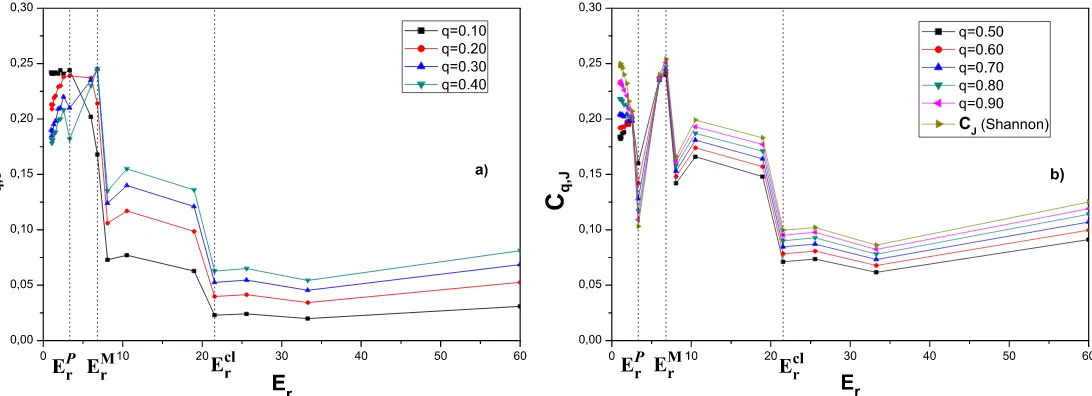
Figure 1. q−Statistical ComplexityCq,J vs. Er forq ≤ 0.4(Fig. 1a) and0.5≤q <1(Fig. 1b). Shannon’s complexity are also displayed. Three zones are to be differentiated. They are delimited by specialEr−values, namely,ErP = 3.3282 andErcl = 21,55264. Notice the local complexity maximum atEM
r ≃6,8155.
0 10 20 30 40 50 60 0,00
0,05 0,10 0,15 0,20 0,25 0,30
E M r E
P r
E cl r
C
q
,
J
E r
q=0.10 q=0.20 q=0.30 q=0.40
a)
0 10 20 30 40 50 60 0,00
0,05 0,10 0,15 0,20 0,25 0,30
b)
E M r
E cl r E
P r
C
q
,
J
E r
q=0.50 q=0.60 q=0.70 q=0.80 q=0.90 C
J
(Shannon)
The first task is to evaluate the set P = {pj} withpj given by (19) [Cf. (11) and (13)]. Our data points are the solutions of (5), from which we extract the values of hx2
i and the (classical) values of
x2
at the time t (for a fixedEr) (We have also performed these calculations extracting instead hp2
i
-p2
together with hLi - L and obtained entirely similar results to those reported below). We will deal with212
data-points, for each orbit. We define eight (NJ = 8) resolution levelsj = −1,−2,· · · ,−NJ for an appropriate wavelet analysis within the multi-resolution scheme of the Appendix . The pj yield, at different scales, the energy probability distribution and in very many instances the NTWE has been found to constitute a suitable tool for detecting and characterizing specific phenomena.
We find, as first result, thatCq,Jcorrectly distinguishes the three zones or sections of our process, i.e., quantal, transitional, and classic, as delimited by, respectively,ErP = 3.3282andErcl = 21,55264, for all values ofq, although the quality of the description steadily worsens forq→ ∞(See Figs. 1, 2, 3, and 4, where we depict Cq,J vs. Er for different q-values). In Fig 1b) we have include the “Shannon case” CJ, i.e., the corresponding wavelet complexity evaluated with the Shannon entropy in (11). Notice the abrupt change of in the slope of the curve taking place at ErP, where a local minimum is detected for
q > 0.2(Fig 1a). The transition zone is clearly demarcated between that point andErcl. From here on Cq,J tends to its classical value at the same time that the solutions of (5) begin to converge towards the classical ones. There are however some transition-details that are not well represented byCq,J, for some
q−values. We thus need to ascertain which is the appropriateq−range.
In general, the most noticeableCq,J−modifications asqvaries take place in the quantal zone, specially forq <1(Figs. 1a-b) and in the transition zone. In the quantum-classic route, an important milestone is found atEr =ErM. This point can be detected, within the transition zone, at the value≈ Er = ErM =
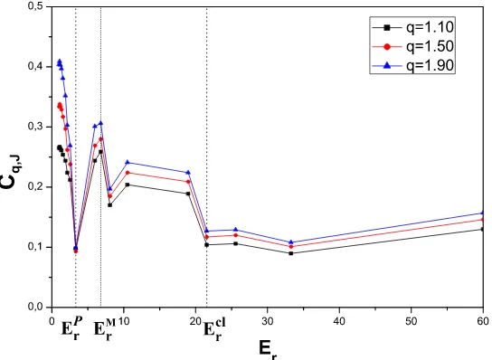
Figure 2. q−Statistical ComplexityCq,J vsErfor1< q <2. The three zones and the point
EM
r of Fig. 1 are also seen here.
0 10 20 30 40 50 60 0,0
0,1 0,2 0,3 0,4 0,5
E
M
r
E cl r E
P r
C
q
,
J
E r
q=1.10 q=1.50 q=1.90
can be verified via Poincare’s sections [34]). EM
r divides into two sections the transitional region, one in which the quantum-classical mixture characterizes a phase-space with more non-chaotic than chaotic curves and other, in which this feature is reversed [34]. The lcm becomes more pronounced asqgrows up toq = 9, and then becomes less and less noticeable, disappearing forq >≈17(Fig. 4).
Notice also that for0.7≤q <1(Fig. 1b) and1< q <2(Fig. 2), ifq →1, theq-complexity behavior resembles more and more the Shannon-one ofCJ. The above picture suffers no great changes forq≥2, save for the above mentioned changes of the local maximum. In view of these considerations, together with the fact that one obviously wishes for aHSq−minimum atE
P
r, we can assert that ourq−quantifiers should be built up inq−range0.2< q ≤17.
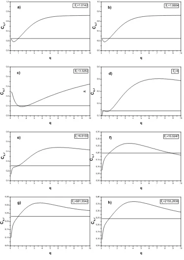
Theq−influence on our transition-processes is clearly appreciated in Figs. 5, that plotsCq,J vs. qfor different values of our all important quantityEr. The corresponding Shannon statistical complexity value (horizontal line) is included in all graphs for comparison’s sake. Figs. 5a)-5b) correspond to the quantum sector, while Figs. 5c), 5d), 5e), and 5f) refer to the transitional one, and, finally, Figs. 5g)-5h) allude to the classical region. AlthoughHSq possesses only one minimum as a function ofq [36],Cq,J instead
may exhibit either a minimum and/or a maximum, plus one or more saddle-points. Consequently, Cq,J intersects Shannon’s curveCJ at least at one point, i.e., i) atq= 1and at one or more points, depending onEr.
We find that distinct quantum-zone’s graphs resemble each other. Ditto for the classical counterparts. Both kinds are clearly different objects, though. See Figs. 5a)-5b) and 5g)-5h), respectively. Moreover, Fig. 5c displays plots corresponding to the neighborhood of ErP point, where the transition region begins to exhibit another kind of morphology. For the transition zone two types of picture can be drawn, corresponding toEr ≤ ErM (with a phase-space with more non-chaotic than chaotic curves) andEr >
EM
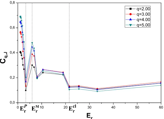
Figure 3. q−Statistical Complexity Cq,J vs. Er for 2 ≤ q ≤ 5. No great changes are observed.
0 10 20 30 40 50 60 0,0
0,2 0,4 0,6 0,8
E P r
E
M
r
E cl r
C
q
,
J
E r
q=2.00 q=3.00 q=4.00 q=5.00
itself, i) of “detecting” important dynamical features like the “Signal Point”ErP and ii) of distinguishing between the two transitional sub-regions, and iii) registering the similarities between the second of these two and the classical one.
5. Conclusions
We have studied in this communication, the classical-quantal frontier of the dynamics governed by a semi-classical Hamiltonian that represents the zero-th mode contribution of an strong external field to the production of charged meson pairs. This study was encompassed within the strictures of the so-called
q−statistics and by recourse to a new tool: theq−Statistical Complexity (13) evaluated by performing a wavelet-band analysis.
The highlights of the road towards classicality are described by recourse to the relative energy Er given by (8). AsErgrows fromEr = 1(the “pure quantum instance”) toEr → ∞(the classical situa-tion), a significant series ofmorphology-changesis detected for the solutions of the system of nonlinear coupled equations (5). The concomitant process takes place in three stages: quantal, transitional, and classic, delimited, respectively, by special values ofEr, namely,ErP andErcl.
We encounter as a first result that Cq,J distinguishes correctly for all value of q, the three sections of our process, i.e., quantal, transitional, and classic, as delimited by, respectively, ErP andErcl. The description suffers a gradual deterioration process asq → ∞, a rather important result in view of the fact that theq−entropyHSq is only able to distinguish our three regions in the range0< q <5. Such a fact
makes theq−Statistical Complexity a much better quantifier than theq−Entropy for the description of a very involved process. As a second we determine an optimalq−rangeO = [0.2< q ≤17], much larger than the above quoted one forHSq. WithinOour complexity-tool distinguishes a valueEr =E
M
r within the transition zone (TZ) in which the complexity exhibits a local maximum. We can partition the TZ at
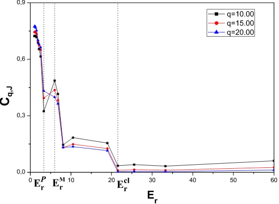
Figure 4. q−Statistical ComplexityCq,J vs. Er for10 ≤ q ≤ 20. The local maximum at
EM
r disappears.
0 10 20 30 40 50 60 0,0
0,3 0,6 0,9
E P r
E
M
r
E cl r
C
q
,
J
E r
q=10.00 q=15.00 q=20.00
thatCq,J, as a function ofqis a good “detector” of transitional features (see Figs. 5): a) it identifiesErP, starting point of the transitional sector, where chaotic behavior begins to emerge and b) it identifiesEM
r , i.e., it distinguishes between the two subsections into which the transitional region divides itself. These last results reconfirm a previous one obtained for HSq in [36], namely, that the parameterqby itself can
be regarded as the “looking glass” through which one can observe the quantum-classical transition.
6. Acknowledgments
AMK are supported by CIC of Argentina. The authors thank Prof. Maria Teresa Martin for her help in the computational aspects.
A Normalized Tsallis wavelet entropy
Wavelet analysis is a suitable tool for detecting and characterizing specific phenomena in time and frequency planes. The waveletis a smooth and quickly vanishing oscillating function with good local-ization in both frequency and time.
Awavelet familyψa,b(t) = |a|−1/2ψ
¡t−b
a
¢
is the set of elementary functions generated by dilations and translations of a unique admissiblemother waveletψ(t). a, b∈ R,a6= 0are the scale and translation parameters respectively, and t is the time. One have a unique analytic pattern and its replications at different scales and with variable time localization.
For special election of the mother wavelet functionψ(t)and for the discrete set of parameters,aj =
2−j andb
j,k = 2−jk, withj, k ∈ Z (the set of integers) the family
ψj,k(t) = 2j/
2
ψ( 2j t − k) j, k ∈ Z , (15)
constitutes an orthonormal basis of the Hilbert spaceL2
(R)consisting of finite-energy signals.
co-Figure 5. q−Statistical Complexity Cq,J for different Er-values. Quantal (Figs. 5a - 5b), transitional (Figs. 5c, 5d, 5e and 5f) and classic (5g - 5h). The curves corresponding to the quantal zone resemble each other and exhibit a different aspect compared to those pertaining to the classical region.
0 1 2 3 4 5 6 7 8 9 10 0,0 0,2 0,4 0,6 0,8 1,0
0 1 2 3 4 5 6 7 8 9 10 0,0 0,2 0,4 0,6 0,8 1,0
0 1 2 3 4 5 6 7 8 9 10 0,0 0,1 0,2 0,3 0,4 0,5
0 1 2 3 4 5 6 7 8 9 10 0,2
0,3 0,4 0,5 0,6
0 1 2 3 4 5 6 7 8 9 10 0,1 0,2 0,3 0,4 0,5 0,6
0 1 2 3 4 5 6 7 8 9 10 0,00 0,05 0,10 0,15 0,20 0,25 0,30 0,35
0 1 2 3 4 5 6 7 8 9 10 0,05 0,10 0,15 0,20 0,25 0,30 0,35
[image:10.595.101.475.184.711.2]efficients provide relevant information in a simple way and a direct estimation of local energies at the different scales. Moreover, the information can be organized in a hierarchical scheme of nested sub-spaces called multiresolution analysis inL2
(R). In the present work, we employ orthogonal cubic spline functions as mother wavelets. Among several alternatives, cubic spline functions are symmetric and combine in a suitable proportion smoothness with numerical advantages.
In what follows, the signal is assumed to be given by the sampled values{x(n), n= 1,· · · , N}. If the decomposition is carried out over all resolutions levels the wavelet expansion will read (NJ = log2(N))
X(t) =
−1
X
j=−NJ
X
k
Cj(k)ψj,k(t) =
−1
X
j=−NJ
rj(t), (16)
whereCj(k)are the wavelet coefficients andrj(t)is thedetail signalat scalej.
Since the family{ψj,k(t)}is anorthonormalbasis forL2(R), the concept of energy is linked with the usual notions derived from Fourier’s theory. The signal energy, at each resolution levelj =−1,· · ·,−NJ, will be the energy of the corresponding detail signal,
Ej = krjk
2
= X
k
|Cj(k)|
2
. (17)
The total energy can be obtained in the fashion
Etot = kXk
2 =
−1
X
j=−NJ
X
k
|Cj(k)|
2 =
−1
X
j=−NJ
Ej . (18)
Finally, we define the normalizedpj-values, which represent therelative wavelet energy
pj = Ej / Etot (19)
for the resolution levelsj =−1,−2,· · · ,−NJ. Thepj yield, at different scales, the probability distri-bution for the energy. Clearly, P
jpj = 1and the distribution {pj}can be considered as a time-scale density that constitutes a suitable tool for detecting and characterizing specific phenomena in both the time and the frequency planes.
The normalized Tsallis wavelet entropy (NTWE) is just the normalized Tsallis entropy associated to the probability distributionP,
HSq[P] =Sq[P]/Sq,max = 1 1−NJ1−q
−NJ
X
j=−1
¡
pj−pqj
¢
, (20)
whereSq,max= (1−N
1−q
energy units) almost equal unity. As a consequence, the NTWE will acquire a very small value. A signal generated by a totally random process or chaotic one can be taken as representative of a very disordered behavior. This kind of signal will have a wavelet representation with significant contributions coming from all frequency bands. Moreover, one could expect that all contributions will be of the same order. Consequently, the relative wavelet energy will be almost equal at all resolutions levels, and the NTWE will acquire its maximum possible value.
References and Notes
1. Shannon, C.E. A mathematical theory of communication. Bell System Technol. J.1948, 27, 379-390.
2. Shiner, J.S.; Davison, M.; Landsberg, P.T. Simple measure for complexity. Phys. Rev. E1999,59, 1459-1464.
3. L´opez-Ruiz, R.; Mancini, H.L.; Calbet, X. A statistical measure of complexity. Phys. Lett. A1995, 209, 321-326.
4. Lamberti, P.W.; Martin, M.T.; Plastino, A.; Rosso, O.A. Instensive entropic non-triviality measure. Physica A2004,334, 119-131.
5. Kolmogorov, A.N.; A new metric invariant of transitive dynamic system and automorphysms in Lebesgue spaces. Dokl. Akad. Nauk SSSR1958,119, 861-864.
6. Sinai, Y.G.; On the concept of entropy of dynamical system. Dokl. Akad. Nauk SSSR1959, 124, 768-771.
7. Mischaikow, K.; Mrozek, M.; Reiss, J.; Szymczak A. Construction of Symbolic Dynamics from Experimental Time Series. Phys. Rev. Lett.1999,82, 1144-1147.
8. Powell, G.E.; Percival, I.C. A spectral entropy method for distinguishing regular and irregular mo-tion of hamiltonian systems. J. Phys A: Math. Gen. 1979,12, 2053-2071.
9. Rosso, O.A.; Mairal, M.L. Characterization of time dynamical evolution of electroencephalographic records. Physica A2002,312, 469-504.
10. Mart´ın, M. T.; Plastino, A.; Rosso, O. A. Statistical complexity and disequilibrium. Phys. Lett. A 2003,311, 126-132.
11. Hanel, R.; Thurner, S. Generalized Boltzmann Factors and the Maximum Entropy Principle: En-tropies for Complex Systems. Physica A2007,380, 109-114.
12. Tsallis, C. Possible generalization of Boltzmann-Gibbs statistics. J. Stat. Phys.1988,52, 479-487. 13. Alemany, P.A. ; Zanette, D.H. Fractal random walks from a variational formalism for Tsallis
en-tropies. Phys. Rev. E1994,49, R956-R958.
14. Tsallis, C. Nonextensive thermostatistics and fractals. Fractals1995,3, 541-547.
15. Tsallis, C. Generalized entropy-based criterion for consistent testing. Phys. Rev. E 1998, 58, 1442-1445.
16. Kalimeri, M.; Papadimitriou, C.; Balasis, G.; Eftaxias, K. Dynamical complexity detection in pre-seismic emissions using nonadditive Tsallis entropy. Physica A2008,387, 1161-1172.
17. Paz, J.P.; Zurek, W.H. Quantum Limit of Decoherence: Environment Induced Superselection of Energy Eigenstates. Phys. Rev. Lett.1999,82, 5181-5185.
two interacting spins. Phys. Rev. E2001,64, 026217:1-026217:11.
19. Kowalski, A.M.; Martin, M.T.; Plastino, A.; Proto, A.N. Classical Limit and Chaotic Regime in a Semi-Quantum Hamiltonian. Int. J. Bifurcation Chaos2003,13, 2315-2325.
20. Kowalski, A.M.; Martin, M.T.; Plastino, A.; Proto, A.N.; Rosso, O.A. Wavelet statistical complexity analysis of the classical limit. Phys. Lett. A2003,311, 180-191.
21. Kowalski, A.M.; Martin, M.T.; Plastino, A.; Rosso, O.A. Entropic Non-Triviality, the Classical Limit, and Geometry-Dynamics Correlations. Int. J. Mod. Phys. B2005,14, 2273-2285.
22. Martin, M.T.; Plastino, A.; Rosso, O.A. Generalized statistical complexity measures: geometrical and analytical properties. Physica A2006,369, 439-462.
23. Bloch, F. Nuclear Induction. Phys. Rev.1946,70, 460-474.
24. Meystre, P.; Sargent, M., III. Elements of Quantum Optics; Springer-Verlag, New York/Berlin, 1991.
25. Bulgac, A. Configurational quasidegeneracy and the liquid drop model. Phys. Rev. C 1989, 40, 1073-1076.
26. Milonni, P.W.; Shih, M.L.; Ackerhalt, J. R. Chaos in Laser-Matter Interactions; World Scientific Publishing: Singapore, 1987.
27. Kociuba, G.; Heckenberg, N. R. Controlling the complex Lorenz equations by modulation. Phys. Rev. E2002,66, 026205:1-026205:5.
28. Ring, P.; Schuck, P.The Nuclear Many-Body Problem; Springer-Verlag, New York/Berlin, 1980. 29. Bonilla, L. L.; Guinea, F. Collapse of the wave packet and chaos in a model with classical and
quantum degrees of freedom. Phys. Rev. A1992,45, 7718-7728.
30. Cooper, F.; Habib, S.; Kluger, Y.; Mottola, E. Nonequilibrium dynamics of symmetry breaking in
λφ4
theory.Phys. Rev. D1997556471-6503.
31. Cooper, F.; Dawson, J.; Habib, S.; Ryne, R. D. Chaos in time-dependent variational approximations to quantum dynamics. Phys. Rev. E1998,57, 1489-1498.
32. Chung, D.J.H. Classical inflaton field induced creation of superheavy dark matter. Phys. Rev. D 2003,67, 083514:1-083514:14.
33. Kowalski, A. M.; Martin, M. T.; Nu˜nez, J.; Plastino, A.; Proto, A. N. A quantitative indicator for semi-quantum chaos. Phys. Rev. A1998,58, 2596-2599.
34. Kowalski, A.M.; Plastino, A.; Proto, A.N. Classical limits. Phys. Lett. A2002,297, 162-172. 35. Kowalski, A.M.; Martin, M.T.; Plastino, A.; Proto, A.N.; Rosso, O.A. Bandt-Pompe approach to
the classical-quantum transition. Physica D2007,233, 21-31.
36. Kowalski, A.M.; Martin, M.T.; Plastino, A.; Zunino, L. Tsallis’ deformation parameter q quantifies the classical-quantum transition. [arXiv:0812.4221v1], 2008;Physica A,2009(in Press).
c