FIA2008-A119
An algorithm for detection and isolation of faulty vibration
modes based on a spectral decomposition of the plant time
response
José Maria Galvez
Department of Mechanical Engineering, Federal University of Minas Gerais, Brazil. Av. Antonio Carlos 6627, Pampulha, 31.270-901 Belo Horizonte, MG, Brazil. E-mail: [email protected]
Abstract
This work presents an algorithm for detection and isolation of faulty vibration modes based on the spectral decomposition of the plant time response. A Hankel matrix is built from plant output measurements and its singular values are used to detect and identify plant parameters related to faulty vibration modes. It is shown that the detection (alarm generation) and isolation (alarm interpretation) tasks are easily performed based on the proposed algorithm. Examples are finally presented to illustrate the performance and application of the proposed algorithm.
Resumen
1 Introduction
The development of safer and more reliable control systems has been an increasingly need in the last decades. To full-fill the modern standards, the control systems design must include fault detection and isolation issues at their very early design stage, Delmaire, Cassar and Staroswiecki (1995), Iserman (1984). The ultimate goal of these systems is to reach a fault-tolerant control (FTC) environment.
Fault detection and isolation (FDI) schemes are implemented as real-time algorithms whose inputs are plant output observations. They are used for a) fault detection: to decide whether the plant is in a normal operating condition or in a faulty one and b) fault isolation: to point out and identify the kind of the fault (if present) among a given fault set. Following the FDI diagnosis, on-line procedures are usually needed for FTC purpose, while off-line procedures could be used for maintenance purpose.
During the last decades, the international scientific community has presented several fine works, Iserman (1984), Yu and Shields (1995). Two main streams can be identified, control related techniques and artificial intelligence based methods. System theory, signal processing or artificial intelligence approaches have been extensively used according to the available data format. Most of the model-based and non-model-based techniques have been developed based on the comparison of the data produced by the real-time plant operation with some previously obtained knowledge of the system.
This paper presents a novel FDI algorithm based on the singular value decomposition of a Hankel matrix built from plant output measurements. The main feature of the proposed algorithm is that it does not rely on plant models. All it is required is a plant signature that can be experimentally obtained. The paper is organized as follows: Section 2 includes some comments on the FDI problem; Section 3 presents the basic formulation of the Eigensystem Realization Algorithm (ERA); Section 4 introduces the singular values based fault detection and isolation (SVFDI) algorithm; Section 5 explores the SVFDI algorithm features through experimental results; and finally, Section 6 presents final comments and conclusions.
2 Some comments on the FDI problem
3 The basics of the Era Algorithm
This section presents the basic formulation of the Eigensystem Realization Algorithm (ERA), as originally proposed by Juang and Pappa in 1985. Since then, the scientific community has proposed several modifications and improvements. The ERA algorithm is a very reliable computational procedure originally proposed for modeling of dynamic systems. For the sake of simplicity and without lost in the argument, this work focuses on the original algorithm. In the following, all posterior algorithm improvements, less important derivation steps and several results have been omitted. Consider a state space realization for a linear time-invariant discrete-time dynamic system given by
) ( ) ( ) ( ) ( ) ( ) ( ) ( ) ( ) 1 ( k v k x C k y k u B k x A k x + = + = + θ θ θ (1)
where, [A, B, C] defines a discrete-time state space realization, x is a n-dimensional state vector, u an m-dimensional control input, y a p-dimensional measurement vector and v represents measurement noise. The system impulse response sequence is given by
B A C k y k
h( +1) = ( +1) = k (2) A Hankel matrix can be constructed from the impulse response sequence as
= + + + + + + + + + = + + + + + + + + . . . . . . . . . . . . . . . . . . . . ) 5 ( ) 4 ( ) 3 ( . ) 4 ( ) 3 ( ) 2 ( . ) 3 ( ) 2 ( ) 1 ( )
( 2 3 4
3 2 1 2 1 B CA B CA B CA B CA B CA B CA B CA B CA B CA k h k h k h k h k h k h k h k h k h k
H k k k
k k k k k k (3) also
[
C
B
B CA B CA B CA B CA B CA B CA B CA B CA CB H = = . . . . . . . . . . ) 0
( 2 3 4
3 2
1
2 1
]
(4)with
[
B AB A B A B]
CA CA CA C n n
B
C
2 11 2 . . & . . − − =
= (5)
where C and B are the observability and controlability matrices, respectively. Also, it should be noted that, usually, H(0) is not square and that dim
(
H(0))
=np Χ nm and. From the singular value decomposition (SVD)
(
H)
n[
n]
T nT
T M D N M I D I N
N M
H 0
0 0
0 0 )
0
(
= = Σ
= (6)
then
B
C
T
Q D P
H(0) = = (7) and
T T QD P
M N
H+ = Σ+ = −1 (8) It is known that, there exist matrices Ep and Em such that
B
C
km T
p H k E H k A
E k
h( +1) = ( ) ; ( )= (9) and that
T
Q D P
H(0) =
C
B
= (10) then[ ]
[ ]
[
]
[
]
[ ][ ]
[ ]
[
pT][
T] [
k T mm T T
T p
m k T p m T
p
E Q D QD
H P D PD E
E DQ QD
k H P D PD E
E A E E k H E k
h
C
B
2 / 1 2 / 1 2
/ 1 2 / 1
1 1
) 1 (
) ( )
( )
1 (
− −
− −
= =
= =
+
]
(11)
finally, a minimal order realization can be found as
[
D 1/2P H(1)QD 1/2]
; B[
D1/2Q E]
& C[
E PD1/2]
A= − T − = T m = pT (12)
Besides that, Juang and Pappa have also proposed two quantitative criteria to eliminate modal frequencies created by measurement noise, Juang and Pappa (1986).
4 The singular values based fault detection and isolation algorithm The proposed SVFDI algorithm can be seen as a generalization of the ERA algorithm (originally applied for model identification). It will be shown later that in the case of the SVFDI problem there is no need for a plant model, all one needs is the singular values of the Hankel matrix built from the plant time response, as shown in the previous section.
values as a measure to detect parametric drift is due to the fact that its nature (real positive numbers) does not change as natural frequencies and eigenvalues do when plant parameters change. Under “normal” operational conditions any change of plant parameters values would affect the system dynamics and in a final analysis the singular values of the Hankel matrix.
In a statistic framework, correlation does not imply causality meaning that correlation cannot be validly used to infer a causal relationship between variables. Consequently, correlation between variables is a necessary but not a sufficient condition to establish a causal relationship. However, having established causality, and in a close-enough neighborhood of the nominal plant, correlation can be taken as the natural choice for analysis. The correlation analysis will deliver a mapping of the plant parameters drifts into the singular values set of the Hankel matrix built from the plant time response. The proposed procedure for fault detection and isolation is depicted in the following section through examples. To illustrate the features of the proposed technique, two lumped parameter models have been chosen as shown next.
5 Experimental results
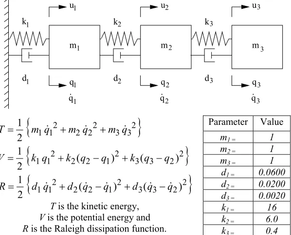
Example I - Let us consider the spring-mass-dashpot system shown in Figure 1.
q1
q2
q3 m1
m2
m3 d1
d2
d3
k1
u1
u2
k2
k3
u3
. q1
. q2
. q3
{
}
{
}
{
2}
3 3 2 2 2 2 1 1
2 3 3 2 2 2 2 1 1
2 3 3 2 2 2 2 1 1
2 1 2 1 2 1
q d q d q d R
q k q k q k
q m q m q m T
& &
&
& &
&
+ +
=
+ +
=
+ +
=
V
T is the kinetic energy,
V is the potential energy and
R is the Raleigh dissipation function. Parameter Value
m1 = 1
m2 = 1
m3 = 1
d1 = 0.0600
d2 = 0.0200
d3 = 0.0020
k1 = 16
k2 = 6.0
k3 = 0.4
Figure 1. The Spring-Mass-Dashpot System for Example I.
Then, the differential equations of motions are given by
3 3 3 3 3 3 3
2 2 3 2 2 2 2
1 1 1 1 1 1 1
u q k q d q m
u q k q d q m
u q k q d q m
= + +
= + +
= +
+
& &&
& &&
& &&
= = = = = + + 1 1 1 & 0 0 0 0 0 0 ; 0 0 0 0 0 0 ; 0 0 0 0 0 0 with 3 2 1 3 2 1 3 2 1 F k k k K d d d D m m m M u F q K q D q M && &
then, a state space representations can be written as
[ ] [ ]
[ ]
[
0]
& 0 ; 0 with ; ; 1 1
1K M D B M F C I
M I A q q x x C y u B x A x = = − − = = = + = − − − & & then = = + − − − − − − = q q x with x y u x x & & 0 0 0 1 0 0 0 0 0 0 1 0 0 0 0 0 0 1 1 1 1 0 0 0 0020 . 0 0 0 4000 . 0 0 0 0 0200 . 0 0 0 0000 . 6 0 0 0 0600 . 0 0 0 0000 . 16 1 0 0 0 0 0 0 1 0 0 0 0 0 0 1 0 0 0
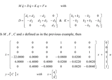
Example II – Let us consider the system presented in Figure 2.
q1 q2 q3
m1 m2 m3
d1 d2 d3
k1
u1 u2
k2 k3
u3
.
q1 q.2 q.3
{
}
{
}
{
2}
2 3 3 2 1 2 2 2 1 1 2 2 3 3 2 1 2 2 2 1 1 2 3 3 2 2 2 2 1 1 ) ( ) ( 2 1 ) ( ) ( 2 1 2 1 q q d q q d q d R q q k q q k q k V q m q m q m T & & & & & & & & − + − + = − + − + = + + =
T is the kinetic energy,
V is the potential energy and
R is the Raleigh dissipation function.
Parameter Value
m1 = 1
m2 = 1
m3 = 1
d1 = 0.0600
d2 = 0.0200
d3 = 0.0020
k1 = 16
k2 = 6.0
[image:6.595.150.449.492.733.2]k3 = 0.4
In this case, the differential equations of motions are given by 3 3 3 2 3 3 3 2 3 3 3 2 3 3 2 3 2 1 2 3 3 2 3 2 1 2 2 2 1 2 2 1 2 1 2 2 1 2 1 1 1 ) ( ) ( ) ( ) ( u q k q k q d q d q m u q k q k k q k q d q d d q d q m u q k q k k q d q d d q m = + − + − = − + + − − + + − = − + + − + + & & && & & & && & & &&
in matrix form, with u1 = u2 = u3 = u , one has
− − + − − + = − − + − − + = = + + 3 3 3 3 2 2 2 2 1 3 3 3 3 2 2 2 2 1 0 0 & 0 0 with k k k k k k k k k K d d d d d d d d d D u F q K q D q M && &
and with M , F , C and x defined as in the previous example, then
[ ]
= = + − − − − − − = q q x with x C y u x x & & 1 1 1 0 0 0 0040 . 0 0020 . 0 0 8000 . 0 4000 . 0 0 0020 . 0 0220 . 0 0200 . 0 4000 . 0 4000 . 6 0000 . 6 0 0200 . 0 0800 . 0 0 0000 . 6 0000 . 22 1 0 0 0 0 0 0 1 0 0 0 0 0 0 1 0 0 0 [image:7.595.105.490.200.477.2]It should be notice that in both examples the plant observability matrix is ill conditioned as shown in Table 1. Despite of that the proposed technique still delivers good results. Table 2 presents the systems eigenvalues and the nominal singular values of the plants.
Table 1. Conditioning Numbers for Examples I and II.
Uncoupled System
Observability Matrix Conditioning Number
Coupled System
Observability Matrix Conditioning Number
2320 . 249
=
γ γ =454.7896
Table 2. System Eigenvalues and Singular Values for Examples I and II.
Uncoupled System
Eigenvalues Coupled System Eigenvalues Uncoupled System Singular Values Coupled System Singular Values
[image:7.595.118.479.546.736.2]Figures 3 through 5 present several dynamic results of the plants used in the Examples I and II. They are placed side by side for comparison purposes.
The Hankel matrix in both cases was built from the impulse responses results shown in Figures 3a and 3b, respectively.
-0.5 0 0.5
T
o: O
ut(
1)
-0.5 0 0.5
To
: O
ut(
2)
0 20 40 60 80 100
-2 -1 0 1 2
To
: O
ut(
3)
Uncoupled System - Impulse Responses
Time (sec)
A
m
plit
[image:8.595.309.525.169.372.2]ude
Figure 3a. Impulse Responses for Example I.
-0.5 0 0.5
T
o: O
ut(
1)
-1 -0.5 0 0.5 1
T
o: O
ut(
2)
0 20 40 60 80 100
-2 -1 0 1 2
To
: O
ut(
3)
Coupled System - Im pulse Responses
Time (sec)
A
m
plit
ud
e
Figure 3b. Impulse Responses for Example II.
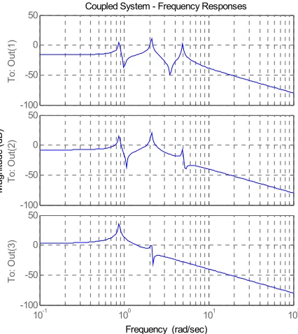
Figures 4a and 4b present the frequency responses for Examples I and II, respectively.
-80 -60 -40 -20 0 20
To
: O
ut
(1
)
-100 -50 0 50
To
: O
ut(
2)
10-1 100 101 102
-100 -50 0 50
To:
O
ut(
3)
Uncoupled System - Frequency Responses
Frequency (rad/sec)
M
agnit
ude (
dB
[image:8.595.61.287.170.375.2])
Figure 4a. Frequency Responses for Example I.
-100 -50 0 50
To
: O
ut(
1)
-100 -50 0 50
To
: O
ut(
2)
10-1
100
101
102
-100 -50 0 50
To
: O
ut(
3)
Coupled System - Frequency Responses
Frequency (rad/sec)
M
ag
nit
ud
e (
dB
[image:8.595.56.273.455.696.2])
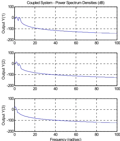
[image:8.595.312.525.456.695.2]Figures 5a and 5b present the power spectrum densities for Examples I and II, respectively.
0 20 40 60 80 100
-200 -100 0 100
O
ut
put
Y
(1)
Uncoupled System - Power Spectrum Densities (dB)
0 20 40 60 80 100
-200 -100 0 100
O
ut
put Y
(2)
0 20 40 60 80 100
-200 -100 0 100
Frequency (rad/sec)
Ou
tp
ut
Y
(3
[image:9.595.314.516.134.370.2])
Figure 5a. Spectrum Densities for Example I.
0 20 40 60 80 100
-200 -100 0 100
O
ut
put
Y
(1)
Coupled System - Power Spectrum Densities (dB)
0 20 40 60 80 100
-200 -100 0 100
O
ut
put
Y
(2
)
0 20 40 60 80 100
-200 -100 0 100
Frequency (rad/sec)
Ou
tp
ut
Y
(3
)
Figure 5b. Spectrum Densities for Example II.
Using standard regression analysis techniques, the correlation coefficients between plant parameters and the singular values of the Hankel matrix were calculated and normalized such that it has been assigned the value of “1” to the greatest coefficient and “0” to the smallest. The results are depicted on Table 3. A “one” would mean strong correlation and a “zeros” a weak or inexistent correlation.
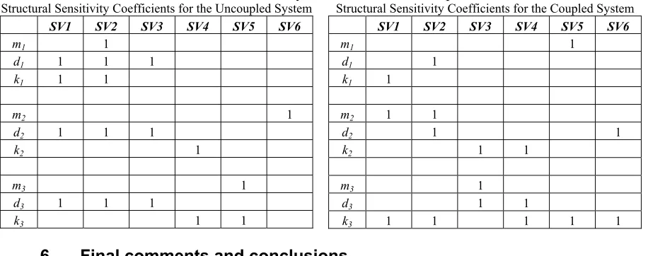
[image:9.595.74.268.134.371.2]Table 3 can be used to select the best singular values to be used as “flags” based on their correlation with plant parameters. From Table 3 one can built Table 4 that presents the structural sensitivity of the singular values with respect to parameter drifts.
Table 3. Correlation Coefficients for Examples I and II.
Correlation Coefficients for the Uncoupled System
SV1 SV2 SV3 SV4 SV5 SV6
m1 0.901 1 0.353 0.082 0 0.077
d1 1 1 1 0.714 0 0.378
k1 0.964 1 0 0.341 0.506 0.592
m2 0.657 0.657 0.657 0.738 0 1
d2 1 1 1 0.655 0 0.204
k2 0.029 0.029 0.029 1 0 0.782
m3 0.200 0.200 0.200 0 1 0.478
d3 1 1 1 0 0.516 0.484
k3 0.102 0.102 0.1 2 0 0.960 1 0
Correlation Coefficients for the Coupled System
SV1 SV2 SV3 SV4 SV5 SV6
m1 0.157 0 0.493 0.424 1 0.905
d1 0.723 1 0.730 0.624 0 0.298
k1 1 0.838 0 0.792 0.931 0.610
m2 1 0.994 0.414 0.361 0 0.391
d2 0.841 0.975 0.604 0.485 0 1
k2 0 0.594 0.993 1 0.644 0.199
m3 0.691 0.710 1 0.405 0 0.864
d3 0.479 0.647 0.999 1 0.409 0
[image:9.595.58.541.542.711.2]Table 4. Structural Sensitivity Coefficients for Examples I and II. Structural Sensitivity Coefficients for the Uncoupled System
SV1 SV2 SV3 SV4 SV5 SV6
m1 1
d1 1 1 1
k1 1 1
m2 1
d2 1 1 1
k2 1
m3 1
d3 1 1 1
k3 1 1
Structural Sensitivity Coefficients for the Coupled System
SV1 SV2 SV3 SV4 SV5 SV6
m1 1
d1 1
k1 1
m2 1 1
d2 1 1
k2 1 1
m3 1
d3 1 1
k3 1 1 1 1 1
6 Final comments and conclusions
This paper presented a fault detection and isolation algorithm based on plant output measurements. In a close neighborhood of the nominal plant values regression analysis has shown to be the proper choice to link the Hankel matrix singular values with plant parameters. An important feature of the SVFDI algorithm is that its formulation does not require a plant model. Having obtained a nominal plant image through the singular values of the Hankel matrix; this image can be used to determine, by comparison, any value drift of the plant parameters. Two functional levels of SVFDI procedure can be distinguished, namely alarm generation and alarm interpretation. At the alarm generation level (detection) the SVFDI algorithm naturally displays plant failure through the change of the singular values structure and values. At the alarm interpretation level (isolation) the SVFDI algorithm delivers an image of the plant parameters through the singular values allowing the identification of the faulty parameter. Finally, the proposed SVFDI algorithm was applied to ill conditioning plants showing outstanding performance in solving both, detection and isolation problems.
7 References
Delmaire, G.; Cassar, J.Ph.; Staroswiecki, M. (1995). “Comparison of Generalised Least Square Identification and Parity Space Techniques for FDI Purpose in SISO Systems”. Proceedings of the 3rd European Control Conference (ECC’95), Rome.
Iserman, R. (1984). “Process Fault Detection Based on Modeling and Estimation Methods, A Survey”. Automatica, vol. 20, pp. 387-404.
Juang, J.N.; Pappa, R.S. (1985). “Eigensystem Realization Algorithm, Journal of Guidance and Control”, vol. 8, n. 3, pp. 620-627.
Juang, J.N.; Pappa, R.S. (1986). “Effects of Noise on Modal Parameters Identified by the Eigensystem Realization Algorithm”. Journal of Guidance and Control, vol. 8, pp. 294-303.
Patton, R.J.; Frank, P.M; Clarck, R.N. (1989). “Fault Diagnosis in Dynamical Systems, Theory and Application”. Prentice-Hall, Englewood Cliffs, NJ, USA.