Robust approaches for fuzzy
clusterwise regression based on
trimming and constraints
Luis Angel Garc´ıa-Escudero1, Alfonso Gordaliza1, Francesca Greselin2, and Agust´ın Mayo-Iscar1
AbstractThree different approaches for robust fuzzy clusterwise regression are reviewed. They are all based on the simultaneous application of trimming and constraints. The first one follows from the joint modeling of the response and explanatory variables through a normal component fitted in each clus-ter. The second one assumes normally distributed error terms conditional on the explanatory variables while the third approach is an extension of the Cluster Weighted Model. A fixed proportion of “most outlying” observations are trimmed. The use of appropriate constraints turns these problem into mathematically well-defined ones and, additionally, serves to avoid the de-tection of non-interesting or “spurious” linear clusters. The third proposal is specially appealing because it is able to protect us against outliers in the explanatory variables which may act as “bad leverage” points. Feasible and practical algorithms are outlined. Their performances, in terms of robustness, are illustrated in some simple simulated examples.
1 Introduction
The detection of clusters around linear subspaces, instead of just around points or centroids, is often needed in Cluster Analysis. This problem is meaningful not only because clusters are frequently arranged this way but also because sometimes it is interesting to discover different relations be-tween a response variable and some other explanatory variables within each cluster. These problems are commonly known as clusterwise linear regres-sion or switching regresregres-sion models. Some others seminal references are [19],
Deptartamento de Estad´ıstica e Investigaci´on Operativa and IMUVA, Universidad de Val-ladolid, ValVal-ladolid, Spain. e-mail: lagarcia,alfonsog,[email protected]·Department of Statistics and Quantitative Methods, Milano-Bicocca University, Milano, Italy. e-mail: [email protected]
[21], [26] and [4]. All those “hard” or 0-1 clustering procedures partition the data intoGcompletely disjoint clusters. Alternatively, fuzzy clustering meth-ods provide nonnegative membership values of observations to clusters and overlapping clusters are so generated [25, 2, 17]. This fuzzy approach can be certainly useful in clusterwise regression applications. There already exist many proposals addressing clustering around linear subspaces problem from a fuzzy clustering point of view. For instance, [17] provides an adaptation of the fuzzy c-means in [2] by minimizing a weighted sum of distances of each observation from the estimated regression line and where these weights de-pend on the fuzzy membership values. See also [18] and [29] and references therein.
Robustness is also a desirable property for (fuzzy) clustering techniques due to the well-know harmful effect that (even a small fraction) outlying observations may have in them. Several methods have been recently proposed to improve clustering techniques robustness performance. For instances, many proposals can be found in [10, 6, 22] (hard) and in [3, 1] (fuzzy).
In this work, we are going to review three recent approaches for robust fuzzy clusterwise regression derived from considering a maximum likelihood approach with trimming and constraints. These methods can see as exten-sions of that introduced in [7]. Trimming is probably the simpler and easier to understand way to achieve robustness. Particularly, we consider an impartial trimming approach where “impartial” means that the data set itself tell us which are observations that should be trimmed as in [9]. When an observa-tion with indexiis detected as an outlier, we set membership valuesuig= 0 for everyg= 1, ..., G. This is in contrast with [29] which setsuig= 1/G for outlying observations. A fuzzy Classification Maximum Likelihood approach is applied in the three considered approaches. The maximization of fuzzified likelihoods is not a new idea in fuzzy clustering [15, 28, 23, 27]. It is impor-tant to fix some type of constraint on the scatters parameters because that maximization is a mathematically ill-defined problem otherwise. Therefore, appropriate constraints on the scatter parameters must be added. These con-straints are also useful to avoid the detection of non-interesting (“spurious”) local maxima.
In the three reviewed methods, the third one is particularly appealing be-cause it simultaneously protects us against “vertical outliers” and even “bad leverage” points. This approach, recently introduced in [13], is a trimmed and fuzzified version of the Cluster Weighted Model (CWM) in [14].
2 Three different approaches
LetXe = (X′, Y)′be a random vector in IRd×IR, where the firstdcomponents X are the values taken by the explanatory variables or covariates, and Y
{(x′i, yi)′}ni=1is a random sample of sizen, drawn fromXe. We use the notation
ϕd(·;m,S) for the density of thed-variate Gaussian distribution with mean
vectorm and covariance matrixSand{λl(S)}dl=1 are the set of eigenvalues of thed×dmatrixS.
2.1 FTCLUST-based approach
The simplest approach follows from the application of the FTCLUST method-ology introduced in [7] in dimension d+ 1. We propose maximizing
n
∑
i=1
G
∑
g=1
umiglog(πgϕd+1(exi;µeg,Σeg)
)
, (1)
where theuig∈[0,1] membership values are required to satisfy
G
∑
g=1
uig= 1 ifi∈ I and
G
∑
g=1
uig= 0 ifi /∈ I, (2)
for a subsetI ⊂ {1,2, ..., n} with #I = [n(1−α)]. The parameterα∈[0,1) is the fixed trimming level and m≥1 is the fuzzifier parameter. Note that observations with indexes outsideI do not contribute to the summation in (1). This target function (1) is unbounded as we can easily seen just by taking|Σeg| →0. Thus, as done in [7], we introduce an additional constraint
when maximizing (1) that forces the set eigenvalues of the scatter matrices to satisfy
λl1(Σeg1)≤cλl2(Σeg2) for 1≤l1̸=l2≤d+ 1 and 1≤g1̸=g2≤G. (3)
This type of constraints are an extension of those in [20, 9]. The use of constraints on the scatter parameters goes back to the seminal work by [16]. Let µeg and Σeg be the vectors and matrices obtained from the previous
constrained optimization problems with
e
µg=
(
µg1
µg2
)
andΣeg=
(
Σg11Σg12 Σg21Σ22g
)
. (4)
From these (optimal) vectors and matrices, we obtainGlinear structures as
y=µg2+Σg21(Σg11)−1(x−µg1) forg= 1, ..., G. (5)
of those in [20, 9]. Some weights πg are also included in (8). We are thus
considering a fuzzy classification EM-type approach as in [28]. These weights are interesting when the number of clusters is misspecified because weights can be set close to 0 wheneverGis larger than needed [9, 7].
The problem with that approach is that linear clusters are generally, by definition, elongated clusters. Therefore, eigenvalues close to 0 on the Σeg
matrices often appear in most of clusterwise regression problems. This fact implies that large c values for the eigenvalues ratio constraint are required. Unfortunately, those largecvalues do not protect us correctly against “spuri-ous” local maximizers. Moreover, the FTCLUST’s good robustness properties are lost with such largecvalues.
2.2 Robust fuzzy clusterwise regression
A different approach, which directly takes into account the underlying lin-ear relations within each group is reviewed in this section. In clusterwise regression, it is frequently assumed that the conditional relation between Y
given X =x in the g-th group can be written as Y = b′gx+b0
g+εg with εg ∼N1(0, σ2
g). In that case, a robust fuzzy clusterwise regression approach
can be derived through the maximization of
n
∑
i=1
G
∑
g=1
umiglog
(
πgϕ1(yi;b′gxi+b0g, σg2)
)
, (6)
where theuigmembership values and theπgweights satisfy the same
require-ments as those in Section 2.1. Vector bg and constant b0g are, respectively,
the regression slopes vector and the intercept for the g-th cluster. Again, constraints on the residual variances can be set as
σg2
1 ≤cεσ
2
g2 for every 1≤g1̸=g2≤G, (7)
for a fixed 1≤cε<∞constant. These constraints again convert the maxi-mization of (6) into a mathematically well-defined problem (see what happens whenσ2
g→0). This approach has been introduced in [11].
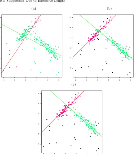
We have applied this methodology, for a simulated data set, with α= 0 and cε= 10 in Figure 1,(a) and with α= 0.05 and cε = 10 in Figure 1,(b). The simulated data set includes a small 5% fraction of background scattered noise. As seen in Figure 1,(a), the detected linear structures whenα= 0 are not the correct ones and many misclassified observations are found.
This approach provides improved robustness performance by applying trimming that certainly protect us against “vertical outliers” (outliers only in
(a) (b)
−2 0 2 4 6 8
−4
−2
0
2
4
6
−2 0 2 4 6 8
−4
−2
0
2
4
6
(c)
−2 0 2 4 6 8
−4
−2
0
2
4
6
Fig. 1 (a) Fuzzy clusterwise regression withα= 0 (b) Fuzzy clusterwise regression with
α= 0.05 (c) Fuzzy robust CWM withα= 0.05 Fuzzy membership values are represented by using a mixture of red and green colors.
points can be extremely harmful in Regression Analysis. Additional protec-tion, in that case, can be obtained by applying a “second trimming” stage as described in [10], which can be straightforwardly adapted to the fuzzy clustering framework.
2.3 Robust fuzzy cluster-weighted model (CWM)
in [14]. This approach has been recently proposed in [13] as a fuzzification of the “hard” robust CWM in [12]. We just focus on the the linear CWM with Gaussian components where the conditional relationship between Y given X=x in theg-th group isY =b′gx+b0
g+εg with εg ∼N1(0, σ2g) but we
also assume thatX∼Nd(µg,Σg).
Under these assumptions, we now consider the maximization of
n
∑
i=1
G
∑
g=1
umiglog(πgϕ1(y;b′gxi+b0g, σ
2
g)ϕd(xi;µg,Σg))
)
, (8)
with the same notation as in the statements of the two previous problems. We have that (8) is unbounded, and consequently, we introduce two further constraints as done in [12]. The first one has to do with the eigenvalues of theΣg matrices throughout
λl1(Σg1)≤cXλl2(Σg2) for every 1≤l1̸=l2≤dand 1≤g1̸=g2≤G.
(9) A second constraint is added on the regression error terms as
σg21 ≤cεσ2g2 for every 1≤g1̸=g2≤G.. (10)
Notice that the two (not necessarily equal) constants 1≤cX <∞and 1≤
cε<∞serve to avoid “spurious” solutions whenever they are not excessively high ones. Moreover, a very flexible methodology is obtained because of the asymmetric treatment given to the marginal and conditional distributions.
Figure 1,(c) shows the results of applying the fuzzy robust CWM with
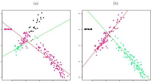
α= 0.05 andcX =cε = 10 for the same simulated data set as above. The methodology in Section 2.2 was perfectly able to recover the two underlying linear structures (recall Figure 1,(b)). However, the cluster assignments are not so satisfactory because some observations which clearly belong to the cluster in the left have higher membership values to the cluster in the right. This issue is due to the fact that they are very close to the regression line fitted by using mainly the observations in the cluster in the right when this line is being elongated. On the other hand, the fuzzy robust CWM take advantage of the information conveyed in the marginalXdistribution and so it is able to obtain more sensible membership values.
CWM, with the same trimming level, succesfully trim bad leverage observa-tions.
(a) (b)
0 2 4 6 8
−2
0
2
4
6
0 2 4 6 8
−2
0
2
4
6
Fig. 2 (a) Robust fuzzy clusterwise regression withα= 0.05 andcε= 10 for a data set with a 5% fraction of concentrated noise (y≃4) (b) Robust fuzzy CWM withα= 0.05 andcX=cε= 10 for the same data set.
3 Algorithms and tuning parameters
In this section, we briefly outline the proposed algorithms to implement the previously reviewed approaches. Note that the target function in all of them can be written as
n
∑
i=1
G
∑
g=1
umiglog(πgφ(exi;θg)), (11)
where function φ(·) and the set of θg parameters change depending on the method applied.
1. Initialization: Initialθg andπgparameters are randomly generated. Small
random subsamples from our original data set are used to obtain these initial parameters.
2. Iterative steps: Repeat the following steps until convergence or reaching a maximal number of iterations:
2.1. Membership values: If maxg=1,...,Gπgφ(xei;θ)≥1,then
uig=I{πgφ(xei;θg) = max
q=1,...,kπqφ(xei;θq)
}
whereI{·}is the 0-1 indicator function. If maxg=1,...,Gπgφ(exi;θg)<1,
we set
uig=
(∑G
q=1
(
log(πgφ(xei;θg))
log(πqφ(xei;θq))
) 1
m−1)−1
. (13)
2.2. Trimmed observations:Compute
ri=
G
∑
g=1
umiglog(pgφg(xi, yi;θ)) (14)
and sort them asr(1)≤r(2)≤...≤r(n). Set membership valuesuig= 0, g= 1, ..., G, for all the indexesisuch thatri< r([nα]).
2.3. Update parameters: Use previousuig to update weights as
πg = n
∑
i=1
umig
/∑n
i=1
G
∑
g=1
umig. (15)
andµg (analogously,µeg) as
µg=
∑n i=1u
m igxi
∑n i=1umig
. (16)
Update intercepts and slope vectors by computing
bg =
(∑n i=1u
m igxix′i
∑n i=1umig
−
∑n i=1u
m igxi
∑n i=1umig
·
∑n i=1u
m igx′i
∑n i=1umig
)−1
·
(∑n i=1u
m igyixi
∑n i=1umig
−
∑n i=1u
m igyi
∑n i=1umig
·
∑n i=1u
m igxi
∑n i=1umig
)
,
and
b0g=
∑n i=1u
m igyi
∑n i=1u
m ig
−b′g
∑n i=1u
m igxi
∑n i=1u
m ig
. (17)
All previous formulae are typical in fuzzy clustering. The most difficult part is how to update the constrained scatter parameters. To update
σ2
g andΣg2, we start from the weighted sample covariance matrices
Tg=
∑n i=1u
m
ig(xi−µg)(xi−µg)′
∑n i=1umig
, (18)
and the weighted residual variances
d2g=
∑n i=1u
m
ig(yi−b0g−x′ibg)2
∑n i=1u
m ig
Then, to update Σg (analogously, Σeg), the singular-value
decomposi-tion Tg =Ug′EgUg is considered, with Ug being an orthogonal matrix
and Eg = diag(eg1, eg2, ..., egd) a diagonal matrix. As done in [8, 7],
these eigenvalues must be optimally truncated. The optimal truncation value is obtained by minimizing a real valued function. Analogously, in case that the d2
j error residual variances do not satisfy the required
constraint, thed2j must be optimally truncated too [11].
3. Return the set ofθg of parameters yielding the highest value of (11) ob-tained after all the random initializations and iterative steps.
Note that trimming is done through “concentration steps” [24] and im-posing the required constraint on the scatter parameters is an important ingredient of this algorithm.
As can be seen, several parameters have to be chosen when applying the proposed methods in real data problems. The estimatedθgparameters do not
necessarily dependent critically on all the tuning parameters. For instance, a trimming level slightly greater than the one needed to remove contami-nation is not necessarily problematic. However, monitoring the sizes of the sorted ri values in (14) is useful to set sensible α values. Regarding the constraints on the scatter parameters, our suggestion is not choosing exces-sively high values for both cX and cε (at least in the approaches described in Section 2.2 and 2.3). The choice of the fuzzifier parameterm depends on the desired degree of fuzziness in the clustering solution. Unfortunately, as happens with other likelihood-based fuzzy clustering approaches, the effect of m is affected by the scale of the measured variables (see [7, 11]). The joint monitoring of the proportions of “hard assignments” and “relative en-tropies” (∑Gg=1∑ni=1uigloguig/[n(1−α)] log(G)) provide useful heuristical tools aimed at addressing this issue.
References
1. Banerjee, A. and Dav´e, R.N. (2012), “Robust clustering,”WIREs Data Mining and Knowledge Discovery,2, 2959.
2. Bezdek, J.C. (1981),Pattern Recognition with Fuzzy Objective Function Algoritms, Plenum Press, New York.
3. Dav´e, R.N. and Krishnapuram, R. (1997). “Robust clustering methods: a unified view”.IEEE Transactions on Fuzzy Systems,5, 270-293.
4. DeSarbo, W.S. and Cron, W.L. (1988). “A Maximum Likelihood Methodology for Clusterwise Linear Regression”,Journal of Classification,5, 249-282.
5. Dotto, F., Farcomeni, A., Garc´ıa-Escudero, L.A. and Mayo-Iscar, A. (2016), “A Fuzzy Approach to Robust Clusterwise Regression,” Accepted for publication inAdvances in Data Analysis and Classification DOI 10.1007/s11634-016-0271-9.
6. Farcomeni, A., Greco, L., (2015)Robust Methods for Data ReductionChapman and Hall/CRC
8. Fritz H, Garc´ıa-Escudero LA, Mayo-Iscar A (2013) “A fast algorithm for robust con-strained clustering”Computational Statistics & Data Analysis,61124–136. 9. Garc´ıa-Escudero, L.A., Gordaliza, A., Matr´an, C. and Mayo-Iscar, A. (2008), “A
general trimming approach to robust cluster analysis”,Annals of Statistics,36, 1324-1345.
10. Garc´ıa-Escudero, L.A., Gordaliza, A., Matr´an, C. and Mayo-Iscar, A. (2010). “A review of robust clustering methods”,Advances in Data Analysis and Classification, 4, 89-109.
11. Garc´ıa-Escudero, L.A., Gordaliza, A., San Mart´ın, R. and Mayo-Iscar, A. (2010) “Ro-bust Clusterwise linear regresssion through trimming.”Computational Statistics and Data Analysis,54, 3057-3069.
12. Garc´ıa-Escudero, L.A., Gordaliza, A., Greselin, F., Ingrassia, S. and Mayo-Iscar, A. (2016) The joint role of trimming and constraints in robust estimation for mixtures of Gaussian factor analyzers,Computational Statistics & Data Analysis,99, 131–147. 13. Garc´ıa-Escudero, L.A., Greselin, F. and Mayo-Iscar, A. (2017) “Robust fuzzy cluster
weighted modeling”,Submitted.
14. Gershenfeld, N., Schoner, B., Metois, E., (1999), “Cluster-weighted modelling for time-series analysis”,Nature,397, 329–332.
15. Gustafson, E.E. and Kessel, W.C. (1979). “Fuzzy Clustering with a Fuzzy Covariance Matrix”.Proceedings of the IEEE lnternational Conference on Fuzzy Systems, San Diego, 1979, 761-766.
16. Hathaway, R. (1985) “A constrained formulation of maximum-likelihood estimation for normal mixture distributions”The Annals of Statistics,13, 795–800.
17. Hathaway, R.J. and Bezdek, J.C. (1993). “Switching regression models and fuzzy clustering”.IEEE Transactions on Fuzzy Systems,1, 195-204.
18. Honda, K., Ohyama, T., Ichihashi, H. and Hotsu, A., FCM-type switching regres-sion with alternating least square method, inProceedings of the IEEE International Conference on Fuzzy Systems (FUZZ 2008), 122-127 (2008).
19. Hosmer, D.W. Jr. (1974), “Maximun Likelihood estimates of the parameters of a mixture of two regression lines.”Communications in Statstics3, 995-1006.
20. Ingrassia S, Rocci R (2007) Constrained monotone EM algorithms for finite mixture of multivariate Gaussians, Computational Statistics & Data Analysis, 51:5339–5351. 21. Lenstra, A.K., Lenstra J.K., Rinnoy Kan, A.H.G., Wansbeek, T.J. (1982) “Two lines
least squares”Annals of Discrete Mathematics16, 201-211
22. Ritter, G. Robust Cluster Analysis and Variable Selection, Chapman & Hall/CRC Monographs on Statistics & Applied Probability, 2015.
23. Rousseeuw, P.J., Kaufman, L. and Trauwaert, E. (1996). “Fuzzy clustering using scatter matrices”.Computational Statistics and Data Analysis,23, 135-151. 24. Rousseeuw, P.J. and Van Driessen, K. (1999), “A Fast Algorithm for the Minimum
Covariance Determinant Estimator,”Technometrics,41, 212-223.
25. Ruspini, E. (1969). “A new approach to clustering”.Information and Control,15, 22-32.
26. Sp¨ath, H. (1982), “A Fast Algorithm for Clusterwise Regression” Computing 29, 175-181.
27. Trauwaert, E., Kaufman, L. and Rousseeuw, P.J. (1991). “Fuzzy clustering algorithms based on the maximum likelihood principle”,Fuzzy Sets and Systems,42, 213-227. 28. Yang, M.-S. (1993). “On a class of fuzzy classification maximum likelihood
proce-dures”Fuzzy Sets and Systems57, 365337.