A Fuzzy Approach to Robust Clusterwise Regression

A Fuzzy Approach to Robust Clusterwise

Regression

Francesco Dotto

,

Alessio Farcomeni

,

Luis Angel

Garc´ıa-Escudero

, and

Agust´ın Mayo-Iscar

1

_{Dipartimento di Scienze Statistiche, Sapienza Universit`}

_{a di Roma}

2

_{Dipartimento di Sanit`}

_{a Pubblica e Malattie Infettive, Sapienza Universit`}

_a

di Roma

3

_{Departamento de Estad´ıstica e Investigaci´}

_{on Operativa, Universidad de}

Valladolid. Valladolid, Spain

Abstract

A new robust fuzzy linear clustering method is proposed. We estimate coefficients

of a linear regression model in each unknown cluster. Our method aims to achieve

robustness by trimming a fixed proportion of observations. Assignments to clusters

are fuzzy: observations contribute to estimates in more than one single cluster. We

describe general criteria for tuning the method. The proposed method seems to be

robust with respect to different types of contamination.

1

Introduction

Many clustering methods are based on estimatekgroups of units according to the distance to

certain applications a different notion of cluster is of interest. For example, in linear

cluster-ing models, k groups of units forming a linear structure are taken in account, which implies

that each unit is assigned to the group minimizing the regression error (i.e. its squared

residuals from the estimated regression line). First attempts to fitk = 2 regression lines can

be found in [18], that applied this type of procedure in economics, in [21] where these type

of procedures are applied in marketing segmentation, and in [27], where the details about

a feasible algorithm are provided. In [26] the EM algorithm has been used in this context

and the methodology has been extended to the multidimensional case and for k > 2. The

general linear clustering method could be then applied in many different research fields like

medicine, psychology, biology, image reconstruction, and many others.

Our aim it to provide a fuzzy linear clustering method that is robust (see e.g. r51 for a

detailed review of the main ideas in robust clustering). We focus on extending the TCLUST

approach. This robust clustering method, that has been proposed in [10], allows the user to

recover heteroscedastic structures and used trimming to avoid the deleterious effect of

outly-ing observations. The extension of this procedure for linear clusteroutly-ing problems appeared in

[11] and, following this idea, we are now interested in extending the robust linear clustering

model proposed in [11] using the fuzzy approach. A review of robust regression can be found

for instance in [16] and [6].

Fuzziness in clustering, that has been introduced in [26] and extended in [14], allows

in-termediate degrees of membership for each observation. It has several advantages in many

applications. In some cases, e.g., [14] or [1], it is not possible to define meaningful hard

par-titions. Our robust fuzzy linear clustering model, based on trimming, also can be seen as an

extension of the method in Hathaway and Bezdeck (see [15] for details). We use a likelihood

based approach with trimming and constraints on the estimated residual variances.

The outline of the paper is as follows: in Section 2 we provide a motivation of the

method-ology and introduce the notation while in Section 3 we report the details of the algorithm

examples. In Section 5 we report a simulation study. Finally Section 6 contains an

appli-cation of our procedure to a real dataset and in Section 7 there are the concluding remarks

and the proposal for further direction of research.

2

Methodology

Let{(yi,x0i)}i=1n ⊂Rp+1 be a dataset wherexi ∈Rpare the values taken by thepexplanatory

variables and yi ∈Ris a continuous response variable for the individuali. Let us suppose to

be interested in grouping them intokclusters in a fuzzy way and estimating a linear model in

each group. Therefore, our aim is twofold: first of all we estimate a set of membership values

uij ∈ [0,1] for all i = 1, ..., n and j = 1, ..., k, where a membership value 1 indicates that

objectibelongs at all to clusterj and conversely a membership value 0 indicates that object

i does not belong to cluster j. Note that intermediate degrees of membership are allowed

when uij ∈(0,1), that implies that an observation gives a contribution in the estimation of

the parameters in each cluster which is proportional to its membership value uij. Secondly

we estimate the regression coefficients and the intercept parameters bj ∈ Rp and b0j ∈ R .

Additionally we consider that an observation is fully trimmed off ifuij = 0 for allj = 1, ..., k

and, thus, this observation has no membership contribution to any cluster. Let: α ∈ [0,1)

be the fixed trimming proportion,c≥1 a fixed constant,m >1 a fixed value of the fuzzifier

parameter, f(·;µ, σ2) the p.d.f of a normal distribution N(µ, σ2) with mean equal to µ and

standard deviation equal to σ. A robust constrained fuzzy linear clustering problem can be

defined through the maximization of the objective function

n

X

i=1 k

X

j=1

um_ij log f(yi;x0ibj+b0j, s 2

j)

(2.1)

where the membership values uij ≥0 are assumed to satisfy

k

X

j=1

uij = 1 ifi∈ I and k

X

j=1

for a subset

I ⊂ {1,2, ..., n}with #I = [n(1−α)],

and and s2

1, . . . , s2k are the residual variances which obey to the constraint:

maxk

j=1s2j

mink_j=1s2 j

≤c. (2.2)

Notice that ui1 =...=uik = 0 for all i /∈ I, so these observations do not contribute to the

summation in the target function (2.1) and these are the trimmed observations.

Using a maximum likelihood criterium like that one in (2.1) implies fixing a specific

under-lying linear model, which indeed allows us to better understand what the fuzzy clustering

method is really aimed at. This maximum likelihood approaches has already been considered,

among others, in [15], [20] and [17].

Another important issue in this approach is to consider, as already done in [11], the

con-straint given in (2.2). In fact, since the target function (2.1) is unbounded, the attempt of

maximizing it without a constraint makes it a mathematically ill posed problem. For instance

we can see that if we take an observationxi and takeb01 and b1 such that yi =b01+x0ib1 then

(2.1) tends to infinity whenever ui1 = 1 and ul1 = 0 for everyl 6=i just by taking s21 →0.

The usage of an objective function like that in (2.1), which does not take in account the

effect of some additional clusters’ weights pj, lends the method a bias toward clusters with

similar sizes (or more precisely toward a solution with similar values of Pk

j=1umij). Then

equation (2.1) may be replaced by:

n X i=1 k X j=1

um_ij log pjf(yi;x0ibj +b0j, s 2

j)

(2.3)

where pj ∈ [0,1] and Pk_j=1pj = 1 are some weights that the objective function also needs

to be maximized on. Notice that, once the membership values are known, these weights are

optimally determined as pj =Pn_i=1umij/

Pn

i=1

Pk

j=1u

m

ij. Thus, this approach implies adding

the term k X j=1 n X i=1

um_ij

log

n

X

i=1

um_ij

n X i=1 k X j=1

um_ij

to the target function (2.1). This type of regularization is related to the “entropy

regular-ization” and appeared in [23]. Note that our objective function (2.3) allow us to consider

the same problem considered in the F-TCLUST approach [7] but in our case, instead of

es-timating robust clusters’ location and scatter parameters in a fuzzy way, we aim to estimate

the parameters yielding a linear model in each fuzzy cluster. Moreover, setting m = 1, we

can state that our procedure is equivalent to the one proposed in [11] without the second

trimming step.

3

The algorithm

Maximization of (2.3) is of course not an easy task. In fact, an iterative procedure which is

able to take in account all the imposed constraints is required. In the following we propose a

computationally feasible algorithm which is supposed to be initialized with several random

starting points and iterates within two alternating steps up to convergence or until a

maxi-mum value of iterations is reached. First, given the values of the parameter at each iteration,

the membership values are obtained. Secondly, given the membership values computed in

the previous step, the parameters are updated in order to maximize (2.3). Therefore we

pro-pose, in order to estimate the regression parameter in all the groups, the adaptation of an

EM-type procedure like those one used in [3] that often appear when fitting finite mixture

of observations [see, e.g., 22]. In any case we can see that the updating formulas for the

membership values and for the parameters are similar to those applied in other fuzzy linear

clustering algorithms like the one proposed in [15], [20] and [17]. Note that, like the whole

procedure may be viewed as an adaptation of [7] for linear clustering, also the algorithm

presents several analogies like, e.g., the application of the constraint (2.2) when the residual

3.1

The proposed algorithm

In this subsection the proposed algorithm is described and briefly commented, while a

step-wise justification follows in the next section.

1 Initialization: The procedure is initialized several times by taking random starting

values p1, . . . , pk, b01, . . . , b0k,b1, . . . ,bk, s21, . . . , s2k. In order to provide these

preliminar-ies estimation k subsets made of p+ 1 observation in general position are randomly

selected and then, the linear systems for estimating the coefficients are resolved and

the associated residual variances are computed. Not that, if required, the estimated

residual variances s2

1, . . . , s2k are constraint in order to satisfy the relation (2.2)

2 Iterative steps: The following steps are executed until convergence or until a maximum

number of iterations is reached.

2.1 Update membership values: Using the current parameter estimates we update the

membership values using following criterium. If

max

q=1,...,k{pqf(yi;x

0

ibq+b0j, s 2

q)} ≥1,

then

uij =I

pjf(yi;x0ibj+b0j, s 2

j) = max

q=1,...,kpqf(yi;x

0

ibj+b0j, s 2

j) (hard assignment)

withI{·} being a 0-1 indicator function which takes the value 1 if the expression

within the brackets holds. If

max

q=1,...,k

pqf(yi;x0ibq+b0q, s 2

q) <1,

then

uij =

k

X

q=1

_log(p

jf(yi;x0ibj +b0j, s2j)

log(pjf(yi;xi0bq+b0q, s2q)

_m1₋₁−1

2.2. Trimmed observations: Let

ri = k

X

j=1

um_ij log(pjf(yi;x0ibj +b0j, s 2

j)) (3.1)

andr(1) ≤r(2) ≤...≤r(n) be these values sorted. The observations to be trimmed

are, at this stage of the algorithm, those with indexes{i:ri < r(dnαe)}. The

mem-bership values for those observations are redefined asuij = 0, for everyj, if ri <

r([nα]).

2.3 Update parameters: Given the membership values obtained in the previous steps,

the cluster weightspj are updated as:

pj =

Pn i=1u m ij Pn i=1 Pk

j=1umij

, (3.2)

while forb0

j and bj, with j = 1,2, . . . , k,the usual (weighted) least square method

is used. Indeed the closed forms for them are

bj =

Pn

i=1umij,x

0

i

Pn

i=1umij −

Pn

i=1uijyi

Pn

i=1umij ·

Pn

i=1umijx

0

i

Pn

i=1umij

Pn

i=1umijx0ixi

Pn

i=1umij −

Pn i=1umijx0i

Pn

i=1uij

2

and b0_j =

Pn

i=1u

m

ijyi

Pn

i=1u

m ij

−b0_j

Pn

i=1u

m

ijxi

Pn i=1u m ij . (3.3)

Updating the s2

j parameters may be more complicate since the weighted sample

residual variances used to update them, given by

d2_j =

Pn

i=1umij(yi−b0j −x

0

ibj)2

Pn

i=1u

m ij

, (3.4)

may not obey to the constraint given by (2.2). In that case, using the procedure

used in [7] for constraining the eigenvalues of the scatter matrices of each cluster

is needed. In order to do that consider the j-th residual variance component dj

and its truncated value which is given by

[d2_j]t=

           d2

j if d2j ∈[t, ct]

t if d2 j < t

ct if d2_j > ct

witht being a threshold value (note that these truncated residual components do

satisfy the required scatter constraint). To define the optimal residual variance

component, an optimal threshold valuetopt is obtained by taking into account the

aim of maximizing the target function (2.3). For instance it can be shown that

topt is the value of t that minimizes the real-valued function:

t 7→

k

X

j=1

pj

log [d2_j]t

+ d

2 j

[d2

j]t

, (3.6)

with pj as defined in (3.2). A closed form to get the value topt exists: indeed

(3.6) must be evaluated in the 2k + 1 points, which are properly defined and

calculated in [8] and [7]. Once these optimal values are properly computed for

each cluster, then the estimated weighted residual variance s2

j can be finally be

updated computings2

j = [d2j]topt.

3 Evaluate the objective function: At the end of the iterative process (i.e. when

conver-gence or a maximum number of iteration is reached) evaluate the value of the associated

target function (2.3). The parameter set yielding the highest value of the objective

function is returned as the output of the algorithm.

3.2

Justification of the algorithm

It can be shown that the two iterative steps of the algorithm increase the value of the target

function (2.3). In one of them, given the regression parameters, we search the membership

values that maximize the target function, while in other one, given the membership values

we estimate the parameter regression and the constraint residual variance parameters that

maximize (2.3). Through this iterative process the algorithm ends up in a local maximum of

(2.3) and by the usage of many random starting points we aim to find the global maximum

of the target function. The rest of this section aims to justify previous claims:

1, . . . , k are known. Maximizing (2.3) is equivalent to minimize n X i=1 k X j=1

um_ijDij (3.7)

where Dij =−log(pjf(yi;x0ibj+b0j, s2j)) = log

p−_j1(2πs2

j)1/2exp (yi−x0ibj −b0j)2/(2s2j)

.

Ifpjf(yi;x0ibj+b0j, s2j)<1 is satisfied for every observationithen the quantity Dij(>0) can

be seen as a measure of the distance of the observed value of the response variableyi from its

fitted valuex0_ibj+b0j. Thus, by the usage of the standard Lagrange multiplier, minimization

of (3.7) with respect to the uij, yields the following optimal membership values

uij = k X q=1 Dij Diq

_m1−1

!−1

,

which coincide with the membership updates of the fuzzy assignments. On the other hand,

if there exist a j such that pjf(yi;x0ibj +b0j, s2j)≥1, that is equivalent to log(pjf(yi;x0ibj+

b0_j, s2_j))≥0 then, in order to maximize (2.3), the crisp assignment proposed is required. To

show that, let us assume that

log(p1f(yi;x0ib1+b01, s 2

1)) = max

j=1,2...,klog(pjf(yi;x

0

ibj +b0j, s 2

j))>0

then the following holds

k

X

j=1

um_ij log pjf(yi;x0ibj+b0j, s 2

j))

≤log p1f(yi;x0ibj +b0j, s

2

j))

k

X

j=1

um_ij

≤log p1f(yi;x0ibj +b0j, s

2 j)) k X j=1

uij = log p1f(yi;x0ib1+b01, s 2

1))

.

and thus we have to impose ui1 = 1 anduij = 0 for every j 6= 1.

Trimmed observations: Within our algorithm a fixed proportionα of observations is allowed

to be discarded. It is straightforward to see that discarding thednαeobservation with lowest

values of the quantity ri defined in (3.1) maximizes our target function (2.3), (indeed our

target function (2.3) may be defined in an alternative way as Pn

i=1ri). This approach to

breakdown point robust statistical procedures (see e.g. [25]).

Parameter estimation: In the parameter estimation step the membership values uij are

supposed to be known from the previous “membership values” and the algorithm aims to

maximize (2.3) with respect to parameters pj, b0j,bj and s2j.

• Clusters weights: Regarding in the pj’s values, it’s straightforward to see that the

quantity proposed in (3.2) is the one needed to maximize (2.3).

• Coefficient’s estimation: In order to estimate the parametersb0

j, andbj, the

minimiza-tion of a weighted least squared funcminimiza-tion is required. Indeed it is straightforward to see

that minimizing the weighted sum of squared residuals between the observed values of

the response variable and the predicted values in each clusters is needed. The weights,

that in this step are considered as known, are represented by the fuzzy assignments of

each observation to each cluster. Formally speaking the required coefficients are the

result of the following minimization:

min

β0

j∈R,βj∈Rp

n X i=1 k X j=1

um_ij(yi−βj0−x

0

iβj)2

for which a closed form for the minimizers is given in (3.3).

• Residual variance estimation: Once that an estimation of pj, b0j,b0j is provided by

applying (3.2) and (3.3) then our aim is to solve the minimization:

min

σ2

1,...,σk2>0

n X i=1 k X j=1

um_ij

1 2log(σ

2

j) +

(yi−b0j −x0ibj)2

2σ2 j

(3.8)

that easily translates into the following problem:

min

σ2

1,...,σ2k>0

k

X

j=1

pj

log(σ2_j) + d

2 j

σ_j2

(3.9)

where indj is the j-th weighted residual variance component defined in (3.2) and the

values σ2

4

Choosing parameters

The methodology described was designed to be as general possible, in order to be useful in

many different applications. A consequence is that there are four choices that the user has

to make: the fuzzifier parameterm, the trimming levelα, the bound on the ratios of residual

variances c, and whether or not including cluster weights (that is, whether or not to shrink

towards approximately balanced clustering).

In this section we investigate the role and the importance of each choice, and give some

guidelines on how to perform each decision in practice. We do so by example, through an

il-lustration based on a simple simulated dataset. We simulate two overlapped two-dimensional

linear clusters. The first cluster is made of 144 observations. The explanatory variable X1i

is generated, as a uniform distribution in the range [0,5], while the response variable is

gen-erated, for each i= 1, . . . , n, as y1i = 1 + 2x1i+ε1i where ε1i ∼ N(0, σ12) and σ1 = 0.4. The

second cluster is made of 216 observations. The independent variableX2i is generated from

a uniform in [0,4] and the response variable as: y2i = 10−1.5x2i+ε2i whereε2i ∼ N(0, σ22)

and σ2 = 0.6. Additional noisy observations are added to our data set as needed.

We now discuss each tuning parameter separately.

4.1

Fuzzifier Parameter

The fuzzifier parametermin equation (2.3) takes values in the range [1,+∞) and it regulates

the degree of fuzziness of the final clustering. Letting m −→ ∞ implies equal membership

values uij = 1/k for every iand for everyj, regardless of the data; while whenm= 1 crispy

weights {0,1} are always obtained and all observations are hard assigned to one and only

one cluster. The optimal value of m depends, as intuitive, on the degree of overlap among

clusters and on how much the researcher is prepared to accept fuzzy weights. Additionally,

a suitable number of hard assignments (or approximately hard assignments) are needed to

the optimal value of m also depends on the scale of the response variable. This issue is a

common problem that affects all the likelihood based fuzzy clustering algorithm like, e.g.

the proposal that appeared in [28] and [24], and at our knowledge, has not been noted so

far in the literature with the exception of [7]. This fact makes it quite difficult to find

reasonable general criteria for choosing m. We illustrate and propose a heuristic procedure

in the following.

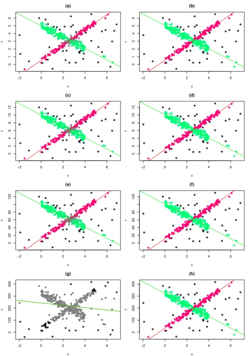
In Figure 1 we applied our procedure to data having different scales for the response variable.

We did so by multiplying the response variable by s ∈ _R+ _{(i.e. y}

i is replaced by yi·s) and

for each scenario we chose two different values for the fuzzifier parameter: m = 1.5, that is

a standard value, and m = 1 that implies no fuzzification in the model. Among the plots

that appear in this Section, in order to graphically represent the fuzzification, we used a

mixture of “red” and “green” colors with intensities proportional to the membership values

of each observations. Additionally, through all the paper, points flagged as outlying under

the model have been represented by “∗” .

Figure 1 shows that when m >1 the scale of the response variable leads to changes in the

results, while whenm = 1 results are scale independent.

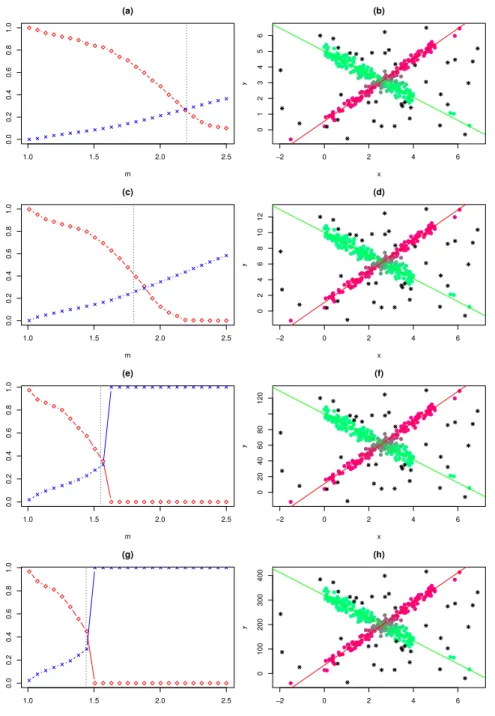
Our proposal for choosingm in practice is to monitor, for each value of m in a pre-specified

grid, two quantities: the proportion of hard assignments and the relative entropy of the

fuzzy weights. The proportion of hard assignments is monitored in order to tunem in order

to obtain a reasonable cluster core for each cluster. The relative entropy measures residual

uncertainty in cluster assignments, and is computed as

Pk

j=1

Pn

i=1uijloguij

[n(1−α)] log(k) . (4.1)

Figure 2 shows the proportion of hard assignments and the relative entropy of the fuzzy

weights as a function of m in our simulated example. We did so by repeatedly applying our

procedure for different values of m. We propose to choose m in order to balance these two

are zero hard assignments and explore the underlying degree of overlap.

−2 0 2 4 6

0 1 2 3 4 5 6 (a) x y

−2 0 2 4 6

0 1 2 3 4 5 6 (b) x y

−2 0 2 4 6

0 2 4 6 8 10 12 (c) x y

−2 0 2 4 6

0 2 4 6 8 10 12 (d) x y

−2 0 2 4 6

0 20 40 60 80 120 (e) x y

−2 0 2 4 6

0 20 40 60 80 120 (f) x y

−2 0 2 4 6

0 100 200 300 400 (g) x y

−2 0 2 4 6

0 100 200 300 400 (h) x y

Figure1: Different degrees of fuzzification obtained for different scale values s∈_R+ _{(see the}

value on the y axis). (a) m = 1.5, s = 0.5. (b) m = 1, s = 0.5. (c) m = 1.5, s = 1. (d)

s = 1, s = 1. (e) m = 1.5, s = 10. (f) m = 1, s = 10. (g) m = 1.5, s = 32. (h) m = 1,

1.0 1.5 2.0 2.5 0.0 0.2 0.4 0.6 0.8 1.0 (a) m

−2 0 2 4 6

0 1 2 3 4 5 6 (b) x y

1.0 1.5 2.0 2.5

0.0 0.2 0.4 0.6 0.8 1.0 (c) m

−2 0 2 4 6

0 2 4 6 8 10 12 (d) x y

1.0 1.5 2.0 2.5

0.0 0.2 0.4 0.6 0.8 1.0 (e) m

−2 0 2 4 6

0 20 40 60 80 120 (f) x y

1.0 1.5 2.0 2.5

0.0 0.2 0.4 0.6 0.8 1.0 (g) m

−2 0 2 4 6

0 100 200 300 400 (h) x y

Figure2: Left panels: relative entropy of the fuzzy weights, “×”, proportion of hard

assign-ments, “”, as a function of scale; (a) s = 0.5. (c) s = 1 (e) s = 10. (g) s = 32. Right

panels: clustering obtained for specific values of m through (b)s = 0.5,m = 2.2. (d)s = 1,

4.2

Including clusters’ weights

In equation (2.1) clusters’ weights have been included. A possibility is to exclude these

weights, with the consequence of shrinking assignments towards an equal number of

obser-vations within each cluster. This is also particularly relevant when the number of clusters is

possibly misspecified.

In Figure 3 we represented a scenario where there are 40% of the clean observations in one

cluster, 60% in the other one, and we estimatedk = 3 clusters. We compare the performance

of the model when the weights are kept in account in the likelihood function, like in equation

(2.3), and when the weights do not appear in the objective function, like in (2.1).

0 1 2 3 4 5

0

2

4

6

8

10

(a)

x

y

0 1 2 3 4 5

0

2

4

6

8

10

(b)

x

y

Figure 3: (a): estimated robust fuzzy clustering when k = 3 and pj are used within the

objective function. (b): estimated robust fuzzy clustering k = 3 and pj are not use within

the objective function.

of the data, indeed, the estimated weights are equal to 0.01,0.42,0.57 (note that one of

them is really close to 0). Note also that two of the three estimated regression lines are

overlapped. On the other hand, when weights are not used estimates of pj correspond to

0.41,0.30 and 0.29, which are clearly biased towards an equal balanced clusters scenario and

two almost parallel clusters are recovered.

4.3

Constraint in the residual variance

An important feature of the proposed algorithm is that no homoscedasticity assumption is

made, or necessary, at all. This is a novel feature as in many switching regression models

(e.g., [15] and [20]) where the residual variance is not kept into account, and implicitly or

explicitly, clusters are assumed to be homoscedastic.

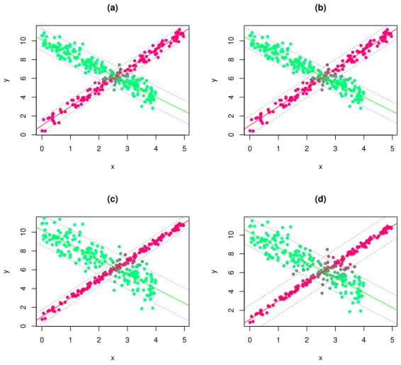
In order to give a brief illustration of how much bias might be obtained by assuming

ho-moscedastic residuals when this assumption does not hold, we compare in Figure 4 estimates

based on c= 1 and c= 5 in two different heteroscedastic scenarios. Recall that fixing c= 1

one forces the residual variances to be equal to each other.

In Figure 4, plot (a), where c = 5, variances are correctly estimated and classification is

very good as only 18 observations out of 360 are wrongly classified. In the other hand, in 4,

plot (b), we run the procedure again on the same data but after fixing c = 1. As could be

expected, variance estimates are pooled. A consequence is that three additional observations

are misclassified.

In panels 4, plot (c) and (d), we repeated this experiment, but with an increased difference

in the underlying variances. In Figure 4, plot (c), wherec= 5, we still have 18 misclassified

observations. In Figure 4, plot (d), where c= 1, we have 32 misclassified observations.

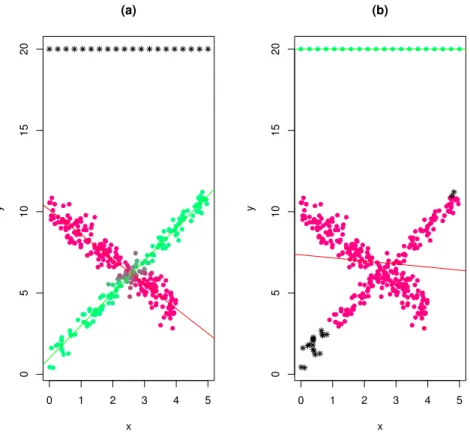
One would be tempted to set a large value for the constraint limitc, but large values might

be associated with spurious maximizers. In the following example we add 20 collinear outliers

that form a spurious cluster and then implement our model withα= 0.05 (that is, requiring

0 1 2 3 4 5

0

2

4

6

8

10

(a)

x

y

0 1 2 3 4 5

0

2

4

6

8

10

(b)

x

y

0 1 2 3 4 5

0

2

4

6

8

10

(c)

x

y

0 1 2 3 4 5

2

4

6

8

10

(d)

x

y

Figure 4: Estimated robust fuzzy clustering for different values of c, σ1 and σ2. (a) c = 5,

σ1 = 0.4 and σ2 = 0.6. (b)c= 1, σ1 = 0.4 and σ2 = 0.6. (c)c= 5, σ1 = 0.2 and σ2 = 1. (d)

c= 1,σ1 = 0.2 andσ2 = 1. The bands are obtained by adding ±2σj to each obtained fitted

regression line.

estimated residual variance to be lower than 5 and once with c = 1010 (basically, without

constraints).

We report the results in Figure 5, where in panel (b), with c = 1010_{, the outliers are not}

discarded. Notably, small groups of collinear observations give an unbounded contribution to

the likelihood if these pathologic solutions are not discarded in advance through appropriate

constraints.

0 1 2 3 4 5

0

5

10

15

20

(a)

x

y

0 1 2 3 4 5

0

5

10

15

20

(b)

x

y

Figure 5: (a): FTCR with c= 5 andα= 0.05. (b): FTCR withc= 1010 _{and α= 0.05.}

thus these observation may not cause a problem in the estimation of the linear structure as

k is properly increased. Nevertheless, since we are assuming that k is fixed in advance, and

we are not aware of the presence of noisy observations, we are mainly interested in providing

the best available solution with respect to the fixed number of groups k. Additionally we

can say that observations having such perfect linear behavior are more likely to come from

another data generating mechanism (i.e. an error in the data registration) and thus they

should be excluded in order to provide meaningful results.

4.4

Setting the trimming level

One of the main innovative features of our approach is that a proportion of observations is

trimmed and does not contribute to clustering or to parameter estimation. More precisely we

having the lowest contributions to the likelihood. The trimming level must be chosen in

advance. There are several methods to do so (see [5] for a deep discussion on this point). In

general, ifα is too low there is an high risk ofmasking, with outliers used for estimation and

loss of robustness. Ifαis too large, there is an high risk ofswamping, with good observations

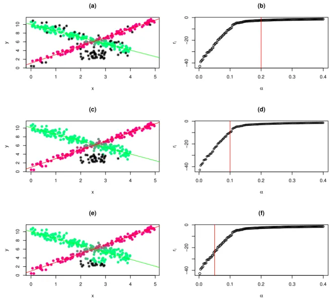
discarded and loss of efficiency. A simple solution that we found effective for robust fuzzy

linear clustering is plotting the average contribution to the likelihoodri against each possible

value of α. We show this in the right panel of Figure 6, and report in the left panel the

estimated linear fuzzy clusters corresponding to the different values ofα. Our proposal is to

fixαas the lowest value after which the average contribution is stable. The idea is that after

all outliers have been removed, the average contribution to the likelihood does not change

much if adding or removing additional observations.

According to our proposal, the optimal value of α would be around 10%. An illustration

of the rationale, based on the figure, follows. Figure 6, panel (a), clearly shows that when

α = 0.2 too many observations have been trimmed. This can be seen also in panel (b) as

the the average contribution to the likelihood has stabilized for much smaller values of α.

On the other hand panel (e) clearly shows that not enough observations have been trimmed.

This can be also seen in panel (f) as the average contribution to the likelihood is much larger

for larger values of α and much smaller for smaller values. Hence, there still are outliers

available for trimming. Finally, α = 0.1, the true underlying contamination level, is a fine

0 1 2 3 4 5 0 2 4 6 8 10 (a) x y

0.0 0.1 0.2 0.3 0.4

−40 −20 0 (b) α ri

0 1 2 3 4 5

0 2 4 6 8 10 (c) x y

0.0 0.1 0.2 0.3 0.4

−40 −20 0 (d) α ri

0 1 2 3 4 5

0 2 4 6 8 10 (e) x y

0.0 0.1 0.2 0.3 0.4

−40 −20 0 (f) α ri

Figure 6: Left panels: Estimated linear clustering result for different trimming levels and

m = 1.5. (a) α = 0.20. (c) α = 0.10. (e) α = 0.05. Right panels: Average contribution to

the likelihood for different values ofα. A red line corresponds to the trimming level used on

the corresponding left panel. (b): α = 0.20. (d): α = 0.10. (f): α= 0.05.

As a concluding remark we would like to point out that a sensitivity analysis, obtained by

varying the tuning parameters in a “proper” range, is always recommended. Additionally

we would like to point out that these proposed heuristic tools can help the user to achieve

sensible tuning of the procedure and that is not necessary to find the exact value for each

the case, very similar results.

5

Simulation study

A simulation study was performed to illustrate and compare our procedure. We simulated 2

overlapped unbalanced linear clusters in two and three dimensions, that is to say that they

are composed, respectively, by p = 1 and p = 2 explanatory variables. The two clusters

were composed of n1 = 144 and n2 = 216 observations, and in the contaminated cases

we added another 40 corrupted observations as described below. Both in two and three

dimensions we had an homoscedastic and an heteroscedastic scenario. In two dimensions

we generated a uniform covariate X1i with support in (0,5) and a uniform covariate X2i

with support in (0,4). The underlying regression models were yi = 1 + 2x1i +ε1i for the

observations within the first cluster and yi = 10−1.5x12+ε2i for the observations within

the second cluster. In three dimensions we generated a uniform covariateX11i with support

in (0,5), another denoted with X12i with support on (5,9), a third (X21i) with support

on (0,6) and, finally, X22 being an independent replica of X12i. The underlying regression

models were yi = 3 + 4x11i −2x12i +ε1i for the observations within the first cluster and

yi =−2−2x12i+ 2x22+ε2i.The errorsε1i and ε2i were zero-centered normals with standard

deviation σ1 and σ2, respectively, where σ1 = 0.4, and σ2 = 0.8 in the heteroscedastic case,

and σ1 =σ2 = 0.4 in the homoscedastic case.

We then considered four contamination’s scenarios:

• Clean dataset

• 10% contaminated dataset with contaminating points generated by sampling from a

uniform distribution in the range of the data

• 10% contaminated dataset with contaminating points generated by sampling from a

• 10% contaminated dataset with pointwise contamination. For instance, in the case of

p= 1 explanatory variable, we generated the contamination jittering around the point

(−1.5,17), while, in the case of p = 2 explanatory variables, the contamination has

been generated by jittering around the point (1,−1.5,18.5).

Therefore we have sixteen different data generating scenarios. Within the outlined scenarios

we implemented the following different models:

1. The proposed fuzzy regression method based on the unconstrained EM algorithm and

without the trimming step. This is the counterpart of our approach. It has been

de-noted in the plot with the acronym “EM” because it would ben the standard adaptation

of the EM algorithm to the fuzzy framework.

2. Our proposed robust Fuzzy TCLUST Regression method, denoted in the plot with the

acronym “FTCR”.

3. The c-Regression model proposed in [15], which has been denoted in the plot with the

acronym “cReg”.

4. The Alternative switching Regression model proposed in [20], which has been denoted

in the plot with the acronym “A-cReg”.

It shall be noted that two of these procedures (EM and cReg) do not take into account

robustness issues, while the other two (A-cReg and our proposed FTCR) do.

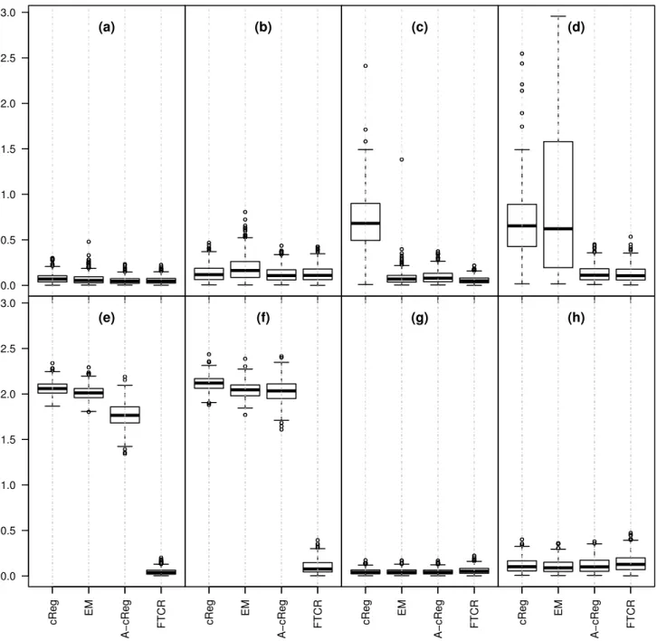
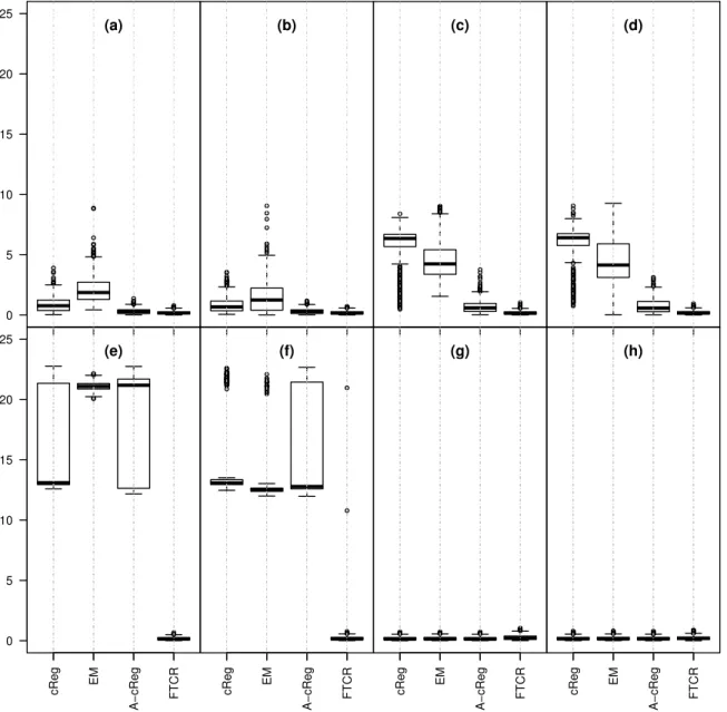
In our simulation study for each scenario we generated the data and estimated the four

models above. We repeated this 500 times and report boxplots of the Mean Squared Error

(MSE) for the slope and the intercept estimators in Figures 7 and 8 when p = 1 and

p = 2, respectively (we stored the obtained estimations in a vector and compared it with

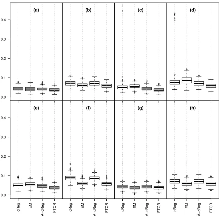
the vector of the real values). Additionally, in Figures 9 and 10 we report boxplots of the

misclassification rates when p= 1 andp= 2, respectively.

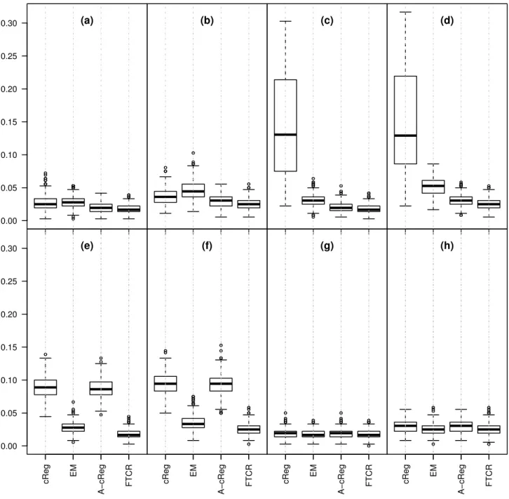
First of all, it can be seen that the procedures have more or less the same performance under

being only slightly worse than the other ones. This is the loss of efficiency which is expected

for any robust procedure, and it is in our opinion very reasonable. On the other hand,

in contaminated scenarios non-robust procedures break down, showing very large MSEs

(especially in scenarios (e) and (f), that are the pointwise contaminated scenarios) and high

variability in performance. On the other hand, FTCR is mostly unaffected by contamination

(a)

0.0 0.5 1.0 1.5 2.0 2.5 3.0

(b) (c) (d)

0.0 0.5 1.0 1.5 2.0 2.5 3.0

cReg EM

A−cReg FTCR (e)

cReg EM

A−cReg FTCR (f)

cReg EM

A−cReg FTCR (g)

cReg EM

A−cReg FTCR (h)

Figure 7: Simulation study: Boxplots representing the MSE of the estimation of βj and b0j

whenp= 1. The Homoscedastic clusters are in (a),(c),(e),(g). Heteroscedastic clusters are in

(b), (d), (f), (h). Uniform contamination is in (a) and (b). Increased uniform contamination

(a)

0 5 10 15 20 25

(b) (c) (d)

0 5 10 15 20 25

cReg EM

A−cReg FTCR

(e)

cReg EM

A−cReg FTCR

(f)

cReg EM

A−cReg FTCR

(g)

cReg EM

A−cReg FTCR

(h)

Figure 8: Simulation study: Boxplots representing the MSE of the estimation of βj and b0j

(a)

0.0 0.1 0.2 0.3 0.4

(b) (c) (d)

0.0 0.1 0.2 0.3 0.4

cReg EM

A−cReg FTCR

(e)

cReg EM

A−cReg FTCR

(f)

cReg EM

A−cReg FTCR

(g)

cReg EM

A−cReg FTCR

(h)

Figure 9: Simulation study. Misclassification error for p= 1 within the same data scenarios

(a)

0.00 0.05 0.10 0.15 0.20 0.25

0.30 (b) (c) (d)

0.00 0.05 0.10 0.15 0.20 0.25 0.30

cReg EM

A−cReg FTCR (e)

cReg EM

A−cReg FTCR (f)

cReg EM

A−cReg FTCR (g)

cReg EM

A−cReg FTCR (h)

Figure 10: Misclassification rates when p = 2 within the same data scenarios outlined in

6

Real Data Example

Allometry studies the relationships between biometric measurements in humans, animals,

and plants. Clusterwise regression is particularly useful for allometric studies since relations

between biometric measurements are often linear or close to linear, possibly after

transfor-mation, and additionally there might be different relationships according to other variables

which might not even be measured. For instance, the relationship between head

circumfer-ence and height in humans is different at different age classes. In our expericircumfer-ence, groups

are seldom perfectly separated and overlapping may hinder the true relationships if not

properly taken into account (e.g., through fuzzy weights). Additionally, outlying biometric

measurements are often present.

We illustrate based on an example already considered in [11], where sharp clusterwise

re-gression was implemented. Here we implement fuzzy clusterwise regression, showing that

use of fuzzy weights leads to better clustering and better understanding of bridge points

between clusters. Data is made of 362 measurements of height and diameter ofPinus Nigra

trees located in the north of Palencia (Spain). We aim to explore the linear relationship

between these two quantities. The scatter plot in Figure 11 clearly shows that there should

be three approximately linear groups, and an isolated group of outliers. This prompted us

to fix k = 3. We applied our procedure twice: once without trimming Figure 11, (a), and

100 200 300

5

10

15

20

25

(a)

diameter

height

100 200 300

5

10

15

20

25

(b)

diameter

height

Figure11: Pinus Nigra Data example. (a) scatter plot and results of the proposed procedure

with no trimming. (b) scatter plot and FTCR with α= 0.04.

It can be seen that the untrimmed procedure is not able to detect the most likely underlying

linear relationships, as the small isolated groups of observations have a direct influence

on one of the clusters, and an indirect one on the other two. A very large coefficient is

estimated for the group including the isolated outliers, while another group includes too

many observations with many fuzzy memberships. On the other hand, by trimming as

few as 15 observations, we recover quite nicely the linear structures. The proportion of hard

assignments is also much larger with FTCR procedure, indicating that the estimated clusters

are well separated. There is also a fair proportion of fuzzy cluster assignments, which might

mislead interpretation if hard assigned (quite arbitrarily) to one of the clusters. In order

plotted in Figure 11 with the symbol “◦”.

Regarding the obtained results a clear explanation for the detected three clusters is that

pines are sampled in three different zones. It can be seen that three almost parallel lines

are obtained, indicating a similar relationship between diameter and height within the three

zones. We can therefore speculate that environmental conditions (e.g., quota, rainfall, sun

exposure) are similar in the three zones, but that immigration of the species has occurred

in different times; where in the “green” zone trees are older (and therefore bigger) and the

most recent colonization (with younger and smaller trees) has occurred in the “blue” zone.

Additionally, outliers can be easily justified: they are trees of a different species originally

misclassified as Pinus Nigra.

We conclude this section by illustrating how we could have chosen the value for the trimming

level α in this example. Although we used the same tuning that has been used in [11], that

is to say that we imposedk = 3 groups and trimming 4% of the observations, a very similar

choice for the trimming level α could have been done by using the heuristical tool proposed

in the previous section. Indeed Figure 12, plot (a), shows how the average contribution to

the likelihood is stabilized when α is set around the value 0.04. In fact even a slightly lower

value could have been chosen and this choice would have avoided trimming the two clean

observation that appear in Figure 11.

Additionally we also had to choose m and we set this parameter equal to 1.3. Indeed, as

it clear from Figure 12, if m > 1.3 the proportion of hard assignments decreases sharply,

0.0 0.1 0.2 0.3 0.4

−60

−50

−40

−30

−20

−10

0

(a)

α

ri

1.0 1.5 2.0 2.5

0.0

0.2

0.4

0.6

0.8

1.0

(b)

m

Figure 12: Pinus Nigra example. (a) average contribution to the likelihood as a function of

α. (b) relative empty entropy and proportion of hard assignments as a function of m.

7

Conclusions and further directions

The proposed procedure is well preforming in terms of robustness, indeed it resists very well

to all the type of contaminations and good efficiency is reached in parameter estimation.

Nevertheless, as often happens in robust procedures, tuning is required in order to have

sensible results. Automatic suitable methods to fix all the tuning parameters, required both

within the robust clustering context and fuzzy clustering methods, are not available yet.

This is not an easy task because all those parameters are interrelated (e.g. a largerα means

that more observations may be discarded and a smaller k value is then needed). However

we shown in Section 4 some heuristical tools that can be useful to help us in tuning all these

References

[1] Ali, Ameer M.; Karmakar, Gour C. nd Dooley, Laurence, S. (2008), “Review on

Fuzzy Clustering Algorithm” Journal of Advanced Computations,2, 169-181.

[2] Bezdek, C.J., and Nikhil, R.P. (1995), “On Cluster Validityfor the fuzzy c-Mean

Model” IEEE transaction on fuzzy systems 3, 370-379

[3] Dempster, A.P., Laird, N.M. and Rubin, D.B. (1977), “Maximum Likelihood from

Incomplete Data via the EM Algorithm,” Journal of the Royal Statistical Society,

Ser. B, 39, 18.

[4] DeSarbo, W.S., Cron, W.L., (1988), “A Maximum Likelihood Methodology for

Clus-terwise Linear Regression” Journal of Classification,5, 249-282

[5] Farcomeni, A., Greco, L., (2015) Robust Methods for Data Reduction Chapman and

Hall/CRC

[6] Farcomeni, A., Ventura, L., (2012). “An overview of robust methods in medical

research” Statistical Methods in Medical Research 21, 111-133.

[7] Fritz, H., Garc´ıa-Escudero, L.A., and Mayo-Iscar, A.(2013). “Robust constrained

fuzzy clustering” Information Sciences 245, 38-52.

[8] Fritz, H., Garc´ıa-Escudero, L.A. and Mayo-Iscar, A. (2012), “A fast algorithm for

robust constrained clustering” Computational Statistics and Data Analysis 61,

124-136.

[9] Gath, I. and Geva, A.B. (1989), “Unsupervised optimal fuzzy clustering.”, IEEE

Transactions on Pattern Analysis and Machine Intelligence,11, 773-781.

[10] Garc´ıa-Escudero, L.A., Gordaliza, A., Matr´an, C. and Mayo-Iscar, A. (2008), “A

general trimming approach to robust cluster analysis”,Annals of Statistics,36,

[11] Garc´ıa-Escudero, L.A., Mayo-Iscar, A. and San Mart´ın R. (2010), “Robust

cluster-wise linear regression through trimming”, Computational Statistics and Data

Anal-ysis,54, 3057-3069.

[12] Garc´ıa-Escudero, L.A., Gordaliza, A., Matr´an, C. and Mayo-Iscar, A. (2011),

“Ex-ploring the number of groups in robust model-based clustering”, Statistics and

Com-puting, 21, 585-599.

[13] Garc´ıa-Escudero, L.A., Gordaliza, A., Matr´an, C. and Mayo-Iscar, A. (2015),

“Avoiding spurious maximizers in mixture modelling”, Stat Comput, 25, 619-633.

[14] Gustafson, E.E. and Kessel, W.C. (1979). “Fuzzy Clustering with a Fuzzy Covariance

Matrix”. Proceedings of the IEEE lnternational Conference on Fuzzy Systems, San

Diego, 1979, 761-766.

[15] Hathaway, R.J. and Bezdek, J.C. (1993). “Switching regression models and fuzzy

clustering”. IEEE Transactions on Fuzzy Systems, 1, 195-204.

[16] Heritier, S., Cantoni, E., Copt, S., and Victoria-Feser, M-P. (2009) Robust methods

in biostatistics Chichester: Wiley

[17] Honda, K., Ohyama, T., Ichihashi, H., and Hotsu, A. (2008), “FCM-type switching

regression with alternating least square method” Proceedings of the IEEE

Interna-tional Conference on Fuzzy Systems (FUZZ 2008),122-127.

[18] Hosmer, D.W. Jr. (1974), “Maximun Likelihood estimates of the parameters of a

mixture of two regression lines.” Communications in Statstics 3, 995-1006.

[19] Kuo-Lung, W., (2012). “Analysis of parameter selections for fuzzyc-means ”Pattern

Recognition

switch-ing regression” Proceedings of the International MultiConference of Engineers and

Computer Scientist 1

[21] Lenstra, A.K., Lenstra J.K., Rinnoy Kan, A.H.G., Wansbeek, T.J. (1982) “Two lines

least squares” Annals of Discrete Mathematics 16, 201-211

[22] McLachlan, G. and Peel, D. (2000), Finite Mixture Models, John Wiley Sons, Ltd.,

New York.

[23] Miyamoto, S. and Mukaidono, M. (1997). “Fuzzy c-means as a regularization and

maximum entropy approach” Proceedings of the 7th International Fuzzy Systems

Association World Congress (IFSA’97),2, 86-92.

[24] Rousseeuw, P.J., Kaufman, L. and Trauwaert, E. (1996). “Fuzzy clustering using

scatter matrices” Computational Statistics & Data Analysis, 23, 135-151

[25] Rousseeuw, P.J. and Van Driessen, K. (1999), “A Fast Algorithm for the Minimum

Covariance Determinant Estimator,” Technometrics, 41, 212-223.

[26] Ruspini, E.H. (1969). “A New Approach to Clustering” Information and Control,

29, 22-32.

[27] Sp¨ath, H. (1982), “A Fast Algorithm for Clusterwise Regression” Computing 29,

175-181.

[28] Trauwaert, E., Kaufman, L. and Rousseeuw, P. (1991), “Fuzzy clustering algorithms