Robust Constrained Fuzzy Clustering
Heinrich Fritza, Luis A. Garc´ıa-Escuderob,∗, Agust´ın Mayo-Iscarb
aDepartment of Statistics and Probability Theory, Vienna University of Technology,
Vienna, Austria
bDepartment of Statistics and Operations Research and IMUVA, University of
Valladolid, Valladolid, Spain
Abstract
It is well-known that outliers and noisy data can be very harmful when ap-plying clustering methods. Several fuzzy clustering methods which are able to handle the presence of noise have been proposed. In this work, we pro-pose a robust clustering approach called F-TCLUST based on an “impartial” (i.e., self-determined by data) trimming. The proposed approach considers an eigenvalue ratio constraint that makes it a mathematically well-defined problem and serves to control the allowed differences among cluster scatters. A computationally feasible algorithm is proposed for its practical implemen-tation. Some guidelines about how to choose the parameters controlling the performance of the fuzzy clustering procedure are also given.
Keywords: Clustering, fuzzy clustering, noise, outliers, constraints, trimming.
1. Introduction
Hard clustering procedures are aimed at searching for a partition of data into k disjoint clusters, with similar subjects grouped in the same cluster and dissimilar subjects in different ones. On the other hand, fuzzy clustering methods provide nonnegative membership values of observations to clusters, and this generates overlapping clusters where every subject is shared among all clusters [see, e.g., 33, 10, 2, 20].
It is also widely recognized that clustering methods need to be robust if they are to be useful in practice. Notice that, otherwise, clustering ability
may deteriorate drastically due to the presence of even a small fraction of outlying data. In fact, historically, the fuzzy clustering community was the first one to face the robustness challenge in Clustering. This is mainly due to the fact that outliers tend to be approximately “equally remote” from all clusters and, thus, they may have similar (but not necessarily small) mem-bership values. For instance, memmem-bership values for outlying observations could be close to 1/k for all the clusters, with k being the number of groups whenever membership values are assumed to sum up to 1. [7] provide a gen-eral review of robust fuzzy clustering methods (see also [15] for a review of robust hard clustering procedures).
One of the methods which is more widely considered in robust fuzzy clustering is the fuzzy C-means method with “noise component” [5] and a plethora of modifications. Unfortunately, this approach inherits its preference for spherical clusters from fuzzyC-means. So, this method is often unable to properly detect clusters with very different shapes. Several procedures have been proposed to address this problem [see, e.g., 18, 17, 34, 31].
In this work, we adapt a hard robust clustering approach called TCLUST [14] to the fuzzy clustering framework. The proposed approach also extends the “Least Trimmed Squares” approach to fuzzy clustering introduced by [21] toward a more general methodology. The proposed methodology is thus based on trimming a fixed fraction α of the “most outlying” observations. We may denote this trimming as “impartial” since the data set itself tells us which are the observations to be trimmed off without the intervention of the user declaring privileged directions or zones for trimming. The fixed trim-ming level controls the number of observations to be discarded in a different way from other methods that are based on fixing a “noise distance” [see, e.g., 6, 8, 29]. These methods are also cited as “noise clustering” in the literature. Discarding a fixed fraction of data has also been considered in [22].
There exist other interesting fuzzy clustering proposals where robustness is incorporated through the replacement of the Euclidean distance as a mea-sure of the discrepancies between observations and cluster centers [35, 25, 37]. However, they are mainly aimed at searching spherical equally scattered groups as fuzzy C-means methods do.
con-straint on the scatter matrices is compulsory because, otherwise, the fuzzy clustering problem would become a mathematically ill-posed problem.
The proposed methodology, called F-TCLUST, is presented in Section 2. A feasible algorithm for its practical application is given in Section 3. The algorithm is theoretically justified in Section 4. Section 5 provides some guidance about how to choose the several parameters that F-TCLUST takes into account. Section 6 presents an application to a well-known real data set. Finally, the paper concludes with some closing remarks and future research lines.
2. The F-TCLUST method
Suppose that we have n observations {x1, ..., xn} in Rp and we want to
group them into k clusters in a fuzzy way. Therefore, our aim is to obtain a collection of nonnegative membership valuesuij ∈[0,1] for alli= 1, ..., nand
j = 1, ..., k. A membership value 1 indicates that object i fully belongs to cluster j while a 0 membership value means that it does not belong at all to this cluster. However, intermediate degrees of membership are allowed when
uij ∈ (0,1). We consider that an observation is fully trimmed if uij = 0 for
all j = 1, ..., k and, thus, this observation has no membership contribution to any cluster.
Let φ(·;µ,Σ) stand for the probability density function of a p-variate normal distribution Np(µ,Σ) defined as
φ(x;µ,Σ) = (2π)−p/2|Σ|−1exp (−(x−µ)′Σ−1(x−µ)/2).
Given a fixed trimming proportionα∈[0,1), a fixed constantc≥1 and a fixed value of the fuzzifier parameter valuem >1; a robust constrained fuzzy clustering problem can be defined through the maximization of the objective function:
n ∑
i=1
k ∑
j=1
umij logφ(xi;mj, Sj), (1)
where the membership values uij ≥0 are assumed to satisfy
k ∑
j=1
uij = 1 if i∈ I and k ∑
j=1
for a subset
I ⊂ {1,2, ..., n} with #I = [n(1−α)],
where m1, ..., mk are vectors in Rp, and, S1, ..., Sk are positive semidefinite
p×p matrices obeying the following eigenvalue ratio constraint
maxk
j=1max
p
l=1λl(Sj)
minkj=1minpl=1λl(Sj)
≤c, (2)
where {λl(S)}pl=1 denote the p eigenvalues of the matrix S.
Notice that ui1 =...=uik = 0 for all i /∈ I, so these observations do not
contribute to the summation in the target function (1).
Using a maximum likelihood criterium like that in (1) implies fixing a specific underlying statistical model, which indeed allows us to better under-stand what the fuzzy clustering method is really aimed at. This maximum likelihood approach has already been considered, among others, in [17], [34], [36], [4] and [31].
One of the main features of the proposed methodology is the application of the eigenvalue ratio constraint in (2). It is important to see that some type of constraint in this maximum likelihood approach is compulsory because, otherwise, the objective function (1) would become unbounded, just by tak-ing one of the mj equal to one of the observations xi, setting uij = 1, and
taking a sequence of scatter matricesSj such that |Sj| →0. This problem is
recurrent in Cluster Analysis whenever general scatter matrices are allowed. For instance, this trouble was already noticed in fuzzy clustering by [18], where they also proposed constraining the relative volumes |Sj| to be equal
to some constants fixed in advance. Other different types of constraint can be found in [34] and [31].
In our approach, the unboundedness problem is addressed by constraining the ratio between the largest and smallest eigenvalues of the scatter matrices. In other words, we are assuming that the square root of the ratio between the lengths of the axes of the tolerance ellipsoids defined through the Sj scatter
with the aim of controlling the cluster shapes. In this work, this constraint on the eigenvalues is explicitly posed in the maximization of the objective function.
The use of an objective function like that in (1) lends the method a bias toward clusters with similar sizes (more precisely toward clusters with similar values of ∑ni=1umij). If this effect is not desired then it is better to replace the objective function (1) by
n ∑
i=1
k ∑
j=1
umij log (pjφ(xi;mj, Sk)), (3)
where pj ∈ [0,1] and
∑k
j=1pj = 1 are some weights that the objective
function also needs to be maximized on. Notice that, once the member-ship values are known, these weights are optimally determined as pj =
∑n
i=1u
m ij/
∑n
i=1
∑k
j=1u
m
ij. Thus, this approach implies adding the term
k ∑
j=1
(∑n
i=1 umij
)
log
(∑n
i=1 umij
/∑n
i=1
k ∑
j=1 umij
)
to the target function (1). This type of regularization is related to the “en-tropy regularizations” [27] which have already appeared in the literature. We will explain, through a simulated data set in Section 5, the impact that the consideration of the weights pj has on the type of clusters we are looking for.
By replacing the target function (1) by (3) in the previously introduced robust constrained fuzzy clustering problem, we obtain the F-TCLUST ap-proach to fuzzy clustering. It is easy to see that it exactly reduces to the TCLUST hard robust clustering method introduced in [14] when the value of the fuzzifier parameter is set at m= 1.
3. A feasible algorithm
Therefore, the algorithm is an “Expectation-Maximization (EM)” type of algorithm [9] as are those often applied when fitting mixtures to data sets [see, e.g., 26]. In any case, we can see that the updating formulas for the membership values and for the parameters are similar to those applied in other fuzzy clustering algorithms when different cluster scatter matrices are allowed (see, e.g., [18] or the algorithms given in [31]).
The algorithm pays special attention to how the constraint on the eigen-value ratios are imposed when updating the Sj matrices in Step 2.3.
More-over, in Step 2.2., the algorithm incorporates a type of “concentration step” analogous to that applied in many high-breakdown point robust algorithms [32]. Note also that the algorithm may be seen as an extension to fuzzy clustering of the TCLUST algorithm in [14] and [12].
Although its proper justification will be deferred to Section 4, the pro-posed algorithm may be described as follows:
1. Initialization: The procedure is initialized several times by randomly selecting parameters p1, ..., pk, m1, ..., mk, and, S1, ..., Sk. For this
pur-pose, we propose to randomly selectk×(p+ 1) observations and to ac-cordingly computekcluster centersmj and scatter matricesSj based on
these chosen data points. If needed, the Sj matrices must be modified
properly so that they satisfy the required eigenvalue ratio constraints by following the approach described in Step 2.3. Weights p1, ..., pk in
the interval (0,1) and summing up to 1 are also randomly chosen. 2. Iterative steps: The following steps are executed until convergence or
a maximum number of iterations is reached.
2.1. Membership values: Based on the current parameters, if
max
q=1,...,kpqφ(xi;mq, Sq)≥1,
then
uij =I{pjφ(xi;mj, Sj) = max
q=1,...,kpqφ(xi;mq, Sq)} (hard assignment),
with I{·} being a 0-1 indicator function which takes the value 1 if the expression within the brackets holds. If
max
then
uij =
(∑k
q=1
(log(p
jφ(xi;mj, Sj))
log(pqφ(xi;mq, Sq))
) 1
m−1)−1
(fuzzy assignment).
2.2. Trimmed observations: Let
ri = k ∑
j=1
umij log(pjφ(xi;mj, Sj)) (4)
and r(1) ≤ r(2) ≤ ... ≤ r(n) be these values sorted. The
observa-tions to be trimmed are those with indexes {i :ri < r([nα])}. The
membership values for those observations are redefined as
uij = 0, for every j, if ri < r([nα]).
2.3. Update parameters: Given the membership values obtained in the previous steps, the parameters are updated as
pj =
∑n
i=1u
m ij
∑n
i=1
∑k
j=1umij
, (5)
and,
mj =
∑n
i=1u
m ijxi
∑n
i=1u
m ij
. (6)
Updating the scatter matrices Sj is more complex, since the
ma-trices that are often used for updating them, defined as
Tj =
∑n
i=1umij(xi−mj)(xi−mj)′
∑n
i=1u
m ij
, (7)
may not satisfy the required eigenvalue ratio constraint. In that case, the singular-value decomposition of Tj = Uj′DjUj is
consid-ered, withUj being an orthogonal matrix andDj = diag(dj1, dj2, ...,
djp) a diagonal matrix. Let us define the truncated eigenvalues as
[djl]t=
djl if djl∈[t, ct]
t if djl< t
ct if djl> ct
with t being a threshold value. The scatter matrices are then updated as
Sj =Uj′D opt j Uj,
with Djopt = diag([dj1]topt,[dj2]topt, ...,[djp]topt
)
where topt
mini-mizes the real-valued function:
t7→
k ∑
j=1 pj
p ∑
l=1
(
log ([djl]t) +
djl
[djl]t )
, (9)
with pj as defined in (5).
In fact, there is a closed form to obtain topt by evaluating the
function (9) 2pk+ 1 times. In order to do that, let us consider the values e1 ≤e2 ≤...≤e2kp obtained after ordering the 2kpvalues:
d11, d12, ..., djl, ..., dkp, d11/c, d12/c, ..., djl/c, ..., dkp/c.
Consider any 2pk+ 1 valuesf1, ..., f2kp+1 satisfying:
f1 < e1 ≤f2 ≤e2 ≤...≤f2kp ≤e2kp < f2kp+1,
and, compute
ti =
∑k
j=1pj(
∑p
l=1djlI{djl< fi}+1c
∑p
l=1djlI{djl> cfi})
∑k
j=1pj(
∑p
l=1(I{djl < fi}+I{djl> cfi})) ,
(10) for i = 1, ...,2kp+ 1. Finally, choose topt as the value of ti which
yields the minimum value of (9).
3. Evaluate objective function: Finally, after this iterative process, the value of the associated target function (3) is computed. The set of parameters and membership values yielding the highest value of this objective function are returned as the algorithm’s output.
The algorithm presented here is focused on maximizing the objective function (3) but it can be easily adapted to perform the maximization of (1) just by assuming fixed equal weights pj = 1/k throughout all the iterations.
imply a higher computational cost (as happens with other closely related algorithms). Experience tells us that not many random initializations and iterations are required when the dimension p is not huge and parameters
m, c, α and k are chosen in a sensible way. Note that the minimization of function (9) does not notably increase the computational complexity of the algorithm.
4. Justification of the proposed algorithm
As previously commented, the proposed algorithm is based on two alter-nating steps. In one of them, we search for the membership values maximiz-ing the target function given the current parameters (Steps 2.1 and 2.2), and, in the other, we search for the parameters maximizing the target function under the constraint on the eigenvalues (Steps 2.3) given the current mem-bership values. The algorithm thus increases the value of the target function through this iterative process, which allows to find a local maximum of the target function (3). The iterative process is randomly initialized several times trying to find the global maximum.
Membership values: Let us assume as known the values of the parameters
pj,mj and Sj. Then, we search for the membership values that make (3) as
large as possible. The maximization of (3) is equivalent to the minimization of
n ∑
i=1
k ∑
j=1
umijDij, (11)
withDij =−log (pjφ(xi;mj, Sk)) = log (p−j1det(Sj)1/2exp((xi−mj)′Sj−1(xi−
mj))).
If we assume thatpjφ(xi;mj, Sj)<1 for allxi, thenDij(>0) can be seen
as a measure of the distances of the observationxi to the center mj (in fact,
exp(Dij) is the “exponential distance measure” introduced in [17]. In this
way, the minimization of (11) on the membership values has a similar state-ment as that considered in fuzzy C-means clustering. Standard Lagrange multiplier arguments lead to optimal membership values as
uij =
( k
∑
q=1
(
Dij
Diq
) 1
m−1
)−1
which indeed coincide with the “fuzzy assignments” proposed in Step 2.1. On the other hand, let us now assume that there exists any j such that
pjφ(xi;mj, Sj) ≥ 1 (that is: log(pjφ(xi;mj, Sj)) ≥ 0). We can assume
w.l.o.g. that log(p1φ(xi;m1, S1)) = maxj=1,..kpjlog(φ(xi;mj, Sj)) ≥ 0 and,
then, we have
k ∑
j=1
umij log (pjφ(xi;mj, Sk))≤log (p1φ(xi;m1, S1))
k ∑
j=1 umij
≤log (p1φ(xi;m1, S1))
k ∑
j=1
uij = log (p1φ(xi;m1, S1)).
Thus, we just need ui1 = 1 and uij = 0 for j ̸= 1 to maximize (3) and the
“hard assignments” proposed in Step 2.1 are justified.
Trimmed observations: When a proportion α of observations is allowed to be discarded, it is quite easy to see that the discarded observations are those yielding the smallest values of ri with ri as defined in (4) to maximize (3)
(recall that (3) is equal to∑ni=1ri). This type of argument is the basis of the
“concentration steps” that some Robust Statistics algorithms apply [32]. The “concentration steps” have been previously used in hard clustering problems [14, 28, 13]. Consequently, the algorithm fixes uij = 0 for all the indexes i
such that ri < r([nα]). This idea also underlies the “Least Trimmed Squares”
approach to fuzzy clustering in [21].
Update parameters: We now assume that the membership values are known and we want to maximize the objective function (3) on the parameters pj,
mj and Sj.
As happens with other maximum likelihood approaches to fuzzy cluster-ing, it is not difficult to see that the best choices for pj and mj are those
given in expressions (5) and (6) [see, e.g., 18, 36]. Plugging these values into (3) and applying the cyclic property of the trace operator, the maximization of (3) can be reduced to the minimization on Sj of
k ∑
j=1
(∑n
i=1 umij
)(
log(det(Sj)) + trace(Sj−1Tj) )
, (12)
Let us consider the spectral decomposition of the matrices Tj =Uj′DjUj
and Sj = Vj′EjVj, with diagonal matrices Dj = diag(dj1, ..., djp) and Ej =
diag(ej1, ..., ejp), and, orthogonal matricesUj and Vj. Mimicking the
reason-ing in [14], it can be shown that the Vj matrix must exactly coincide with
Uj. This tells us that the “shapes” of the optimal matrices Sj are uniquely
determined by the Tj matrices. Therefore, it is only necessary to choose the
optimal eigenvalues eij properly.
By usingUj =Vj and the fact that these matrices are orthogonal, we can
easily see that the minimization of (12) simplifies to the minimization of
k ∑
j=1
(∑n
i=1 umij
)∑p
l=1
(
logejl+
djl
ejl )
, (13)
with ejl taking some values that satisfy the constraint ejl/euv ≤c for every
j, l, uandv. This can be done [see details in 12] by truncating the eigenvalues
djl from below by a constant t and from above by c·t (i.e., considering the
truncated [djl]tgiven in (8)) and searching for the optimalt which minimizes
the real-valued function (9). This function is continuously differentiable and, thus, it attains the minimum value at one of its critical points (with expres-sions like those in (10)).
5. Choice of parameters
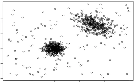
Since the proposed methodology aims to be very general, several parame-ters are involved in it. In this section, we will explain the different roles that the parameters in the F-TCLUST play through a simulated data set. Thus we consider a very simple example made up of 450 random observations in
R2 from the N
2(0, I) distribution and another 450 observations from the
N2
((
5 10
)
,
(
4 −2
−2 4
))
distribution. We also add 100 uniformly distributed observations in the rect-angle [−10,15] × [−10,15], but not considering those observations whose Mahalanobis distances (using the parameters of these two bivariate normal distributions) are smaller thanχ2
2;0.975 (whereχ22;0.975 is the 0.975 quantile of
−10 −5 0 5 10 15
−10
−5
0
5
10
15
Data set
x1
x2
Figure 1: Simulated data set with a 10% noise proportion.
this way, these 100 added observations can actually be considered as a 10% background noise. Figure 1 shows a scatterplot of that simulated data set.
Fuzzifier parameter: We first study the effect of the fuzzifier parametermin the clustering results when applying the F-TCLUST procedure with k = 2,
c = 5 and α = 0.1. Figure 2 shows the obtained cluster membership values by plotting observations with point sizes proportional to these membership values. Trimmed observations are shown in a separate plot.
As previously commented, the m = 1 case coincides with the TCLUST method yielding “hard” or “crisp” membership values, where each obser-vation is fully trimmed or fully assigned to a cluster as shown in Figure 2,(b). On the contrary, all non-trimmed observations are “shared” with al-most equal membership values in Figure 2,(c) when a large value of m, like
m = 2, is chosen. Intermediate values of m, like m = 1.3, surely yield more interesting membership values, as shown in Figure 2,(a).
(a) m=1.3 (Fuzzy clustering)
−10 −5 0 5 10 15
−10 −5 0 5 10 15
Cluster 1
x1
x2
−10 −5 0 5 10 15
−10 −5 0 5 10 15
Cluster 2
x1
x2
−10 −5 0 5 10 15
−10 −5 0 5 10 15 Trimmed x1 x2
(b) m=1 (Hard clustering)
−10 −5 0 5 10 15
−10 −5 0 5 10 15
Cluster 1
x1
x2
−10 −5 0 5 10 15
−10 −5 0 5 10 15
Cluster 2
x1
x2
−10 −5 0 5 10 15
−10 −5 0 5 10 15 Trimmed x1 x2
(c) m=2 (Too much fuzziness)
−10 −5 0 5 10 15
−10 −5 0 5 10 15
Cluster 1
x1
x2
−10 −5 0 5 10 15
−10 −5 0 5 10 15
Cluster 2
x1
x2
−10 −5 0 5 10 15
−10 −5 0 5 10 15 Trimmed x1 x2
clusters.
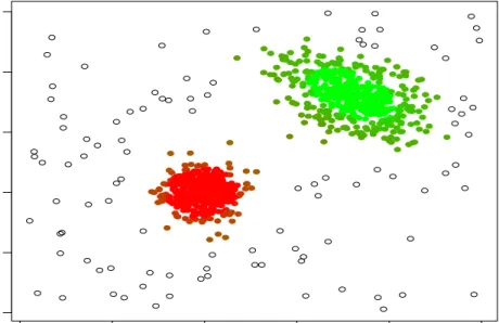
It is also important to pay special attention to an inherent problem of fuzzy clustering approaches based on the maximum likelihood principle. To see this, let us assume that the variables in our example are scaled by a constant factor S. That is, we change the variables as follows: X1 ← X1/S
and X2 ← X2/S . Figure 3,(a) shows that m = 5 yields a very high degree of fuzzification (in fact, m = 2 already did so). However, a logical degree
−10 −5 0 5 10 15
−10
−5
0
5
10
15
(a) S = 1
x1
x2
−1.0 −0.5 0.0 0.5 1.0 1.5
−1.0
−0.5
0.0
0.5
1.0
1.5
(b) S = 10
x1
x2
−0.04 0.00 0.04
−0.04
0.00
0.02
0.04
0.06
(c) S = 200
x1
x2
−10 −5 0 5 10 15
−10
−5
0
5
10
15
(d) S = 1
x1
x2
−1.0 −0.5 0.0 0.5 1.0 1.5
−1.0
−0.5
0.0
0.5
1.0
1.5
(e) S = 10
x1
x2
−0.04 0.00 0.04
−0.04
0.00
0.02
0.04
0.06
(f) S = 200
x1
x2
of fuzzification is obtained in Figure 3,(b) with m = 5 when the variables are scaled with an S = 10 factor. Finally, we obtain a hard clustering partition of the data set with the same value m = 5 when S = 100 in Figure 3,(c). In these figures, we use a mixture of “red” and “green” colors with intensities proportional to the membership values to summarize the fuzzy clustering results, while trimmed points are always represented by “◦” symbols. This dependence on the scale factorSno longer appears when using a hard clustering approach (i.e. whenm= 1), as can be seen in Figures 3,(d), (e) and (f).
The clustering results shown in Figure 3,(b) (augmented in Figure 4) are particularly interesting. We can see that “hard” assignment decisions are made in the “core” of the clusters, with observations that are undoubtedly assigned. “Fuzzy” assignments are made for the observations that are more difficult to be classified in the tails of the two normal components. These two different types of assignment decisions follow from the application of Step 2.1 in the proposed algorithm. This naturally leads to a fuzzy clustering method with “high contrast” [30]; that is, it may be seen as a compromise between “hard” and “fuzzy” clustering methods. If “high contrast” partitions are specially interesting for the user, then this provides an appropriate way to
−1.0 −0.5 0.0 0.5 1.0 1.5
−1.0
−0.5
0.0
0.5
1.0
1.5
x1
x2
scale the data by determining S in such a way that a fixed proportion of “hard” assignments are done.
Weights and number of clusters: The addition of weights pj in expression
(3) (instead of considering (1)) is very important. We are “ideally” assuming that the clusters have similar sizes when weights pj do not appear in the
target function to be maximized. This does not necessarily imply that the resulting clusters satisfy ∑ni=1umi1 = ... = ∑ni=1umik, but we are “ideally” searching for this type of clustering solutions, and not very interested in clustering solutions too far from that case.
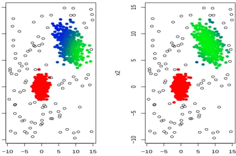
We can see in Figure 5,(a) the clustering results fork = 3,c= 5, α= 0.1 and m = 1.3 when maximizing (1) (that is: “equal weights”) and when maximizing (3) in Figure 5,(b) (that is: “unequal weights”). The clustering solution in Figure 5,(b) is essentially made up of just two clusters, while the third cluster has small membership values for all observations. In this example, k = 2 is clearly a good choice for the number of clusters (once 10% of the outlying data points are trimmed). Thus, the fact of allowing for weightspj in the target function could provide interesting information about
−10 −5 0 5 10 15
−10
−5
0
5
10
15
(a)
x1
x2
−10 −5 0 5 10 15
−10
−5
0
5
10
15
(b)
x1
x2
how to make sensible choices for k. This possibility was already considered in hard clustering problems in [16].
Note also that Figure 5,(a) shows many intermediate membership values due to the clear overlap between the two clusters that share one of the two normal components. This “soft” transition between clusters is only feasible when applying fuzzy clustering techniques.
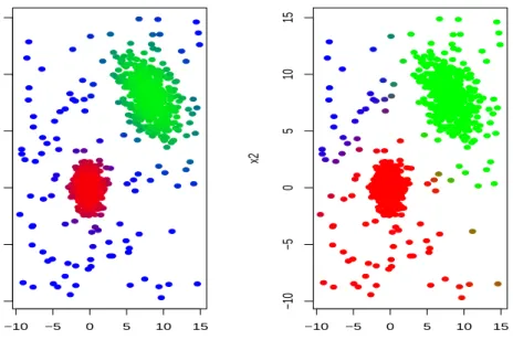
Eigenvalue ratio restriction constant: One of the most distinctive features of the proposed F-TCLUST approach is the consideration of constraints on the cluster scatters following from the control of relative sizes of the scatter matrix eigenvalues through constant c. For instance, we allow for clusters with very different scatters in Figure 6,(a) when fixing a large c value (like
c= 50). This has allowed for the detection of a very scattered group (shown in “blue” color). On the other hand, the clusters are forced to have very similar scatters when c = 1, as shown in Figure 6,(b). In this second case, the more scattered cluster is no longer possible. Moreover, whencis close to 1, the clusters are forced to be almost spherical (and with the same scatter among them) and, thus, F-TCLUST may be seen as an extension of the fuzzy
C-means method.
−10 −5 0 5 10 15
−10
−5
0
5
10
15
(a)
x1
x2
−10 −5 0 5 10 15
−10
−5
0
5
10
15
(b)
x1
x2
With respect to the choice of parametercin a specific clustering problem, the researcher sometimes has an initial idea of the differences between group scatters that he/she is willing to accept, depending on the application in mind for the clustering results. When such information is not available, we propose to monitor the sequence of clustering solutions obtained when moving c. In our experience, not too many essentially different clustering solutions need to be evaluated. The interpretation of c in terms of the lengths of the axes of the ellipsoids defined by the Sj matrices will be very important in this
process. It is also informative to check whether the resulting Sj matrices
satisfy λl(Sj) = λv(Su) for some (l, j)̸= (v, u) or not, to see if the algorithm
is “artificially” forcing the fulfillment of the required constraints for a given value of constant c.
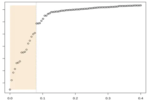
Trimming level: Another parameter that plays a key role in the F-TCLUST methodology is the trimming level α. Recall that observations are fully declared as noise when they are trimmed and no “intermediate” noise as-signments are allowed (as, for instance, the methods based on the “noise clustering” approach do).
Sometimes, the researcher has an approximate initial idea of the under-lying “contamination level” in the data set, but at other times this con-tamination level is completely unknown. In the case where this underlying contamination level is unknown, we can see that monitoring the ri values
introduced in (4) provides valuable information to see whether the choice made for α was sensible or not. Recall that these values are used to deter-mine the trimmed observations as long as outlying observations take small
ri values. Thus, for a tentative trimming level α, we propose plotting the
points {(i/n, r(i))}i=1,2,3,... obtained with F-TCLUST for this value of α.
Re-call that r(1) ≤ ... ≤ r(n) are the sorted ri values. The choice made for α
is considered as being appropriate if it is close to a value α0, such that the
values r(i) increase quickly when i/n < α0 and the increase becomes slower
when i/n > α0.
For instance, in Figure 7,(b), (d) and (f), we have plotted theser(i) values
for α = 0.02,0.2 and 0.1. The value α = 0.02 is clearly not a good choice because the r(i)values are still increasing quickly at this value ofα, as can be
−10 −5 0 5 10 15
−10
−5
0
5
10
15
(a)
x1
x2
0.0 0.1 0.2 0.3 0.4
−80
−60
−40
−20
(b)
Trimming level alpha
r_i
−10 −5 0 5 10 15
−10
−5
0
5
10
15
(c)
x1
x2
0.0 0.1 0.2 0.3 0.4
−30
−25
−20
−15
−10
−5
(d)
Trimming level alpha
r_i
−10 −5 0 5 10 15
−10
−5
0
5
10
15
(e)
x1
x2
0.0 0.1 0.2 0.3 0.4
−60
−40
−20
(f)
Trimming level alpha
r_i
Figure 7: Different clustering solutions depending on the chosen trimming level (α = 0.02,0,2 and 0.1) and the plots of the sortedri values for each different choice ofα.
this simulated data set.
It is not compulsory to be extremely precise with an “exact” choice of α
because the parameters pj, mj and Sj do not change notably, for instance,
it is not difficult to make a better choice for the trimming level by carefully analyzing the trimmed observations which are close to the non-trimmed ones. From our point of view, in general, it is recommended to be initially conser-vative when choosing α.
We are currently investigating the possibility of unsupervised methods for choosing the trimming levelα. However, it is important to note that the problem of choosing α is closely related to the choice of parameters k and c
[see 16]. Addressing all these determinations in a unified manner still requires an active role to be played by the researcher, as a final decision may be very subjective, and, thus, it is not clear that a fully unsupervised strategy can be found.
To clarify previous claims, let us consider again the data set in Figure 1. If we allow for a large value of c (i.e., huge differences among cluster scatters), then k = 3 andα = 0 is a sensible choice. But, on the other hand, it is surely better to choose k = 2 and α = 0.1 when c is small. The fuzzy adaptation of the “classification trimmed-likelihood curves” introduced in [16] might be considered as an exploratory tool to help the researcher make sensible simultaneous choices for k,α and c(see Section 7).
Another possibility that may be explored follows from monitoring some cluster validity index [e.g., the density criterion in 17] against the trimming level α, as proposed in [21].
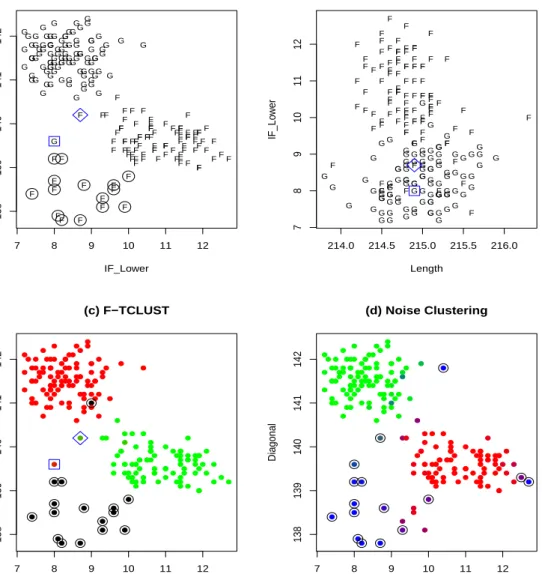
6. A real data example
The “Swiss Bank Notes” data set in [11] includesp= 6 variables measur-ing certain features in the printed image of 100 genuine and 100 counterfeit old Swiss 1000-franc bank notes.
also show an observation surrounded by a “” symbol that corresponds to a “genuine” bill that would fit better in the group of “forged” bills [see 11].
G G G G G G G G G G G G G G G G G G G G G G GG G G G G G G G G G G G G G G G G G G G G G G G G G G G G G G G G G G GG G G GG G
G G G G G G G G G G G G G G G G G G G G G G G G G G G G G G G G G G G F F F F F F F F F F F F F F F F F F F F F F F F F F F F F F F F F F F F F F F F FF F F F F F F F F F F F F F F F F F F F F F F F F F F F F F F F F F F F F F F F F F F F F F F F F F F F F F F F F F F
7 8 9 10 11 12
138
139
140
141
142
(a) True classification (4th vs. 6th)
IF_Lower Diagonal G G G G G G G G G G G GG G G G G G G G G G G G G G G G G G G G G G G G G G G G G G G G G G G G G G G G G G G G G G G G G G G G G G G G G G G G G G G G G G G G G G G G G G G G G G G G G G G G G G G G F F F F F F F F F F F F F F F F F F F F F F F F F F F F F F F F F F F F F F F F F F F F F F F F F F F F F F F F F F F F F F FF F F F F F F F F F F F F F F F F F F F F F F F F F F F F F F F F F F F F
214.0 214.5 215.0 215.5 216.0
7 8 9 10 11 12
(b) True classification (1st vs. 4th)
Length
IF_Lo
w
er
7 8 9 10 11 12
138 139 140 141 142 (c) F−TCLUST IF_Lower Diagonal
7 8 9 10 11 12
138
139
140
141
142
(d) Noise Clustering
IF_Lower
Diagonal
Figure 8,(c) shows the F-TCLUST clustering results with parametersk= 2, α = 0.08, m = 1.3 and c = 10. Membership values are summarized by using a mixture of “red” and “green” colors and the trimmed observations are shown as “black points” surrounded by circles. Taking into account the prior knowledge of the existence of 15 + 1 “anomalous” bills, we have chosen
α = 0.08 (which yields 200·0.08 = 16 trimmed observations). We can see that the genuine bills are clustered into the “red” cluster and the forged ones into the “green” cluster. Apart from one wrongly trimmed genuine bill, the F-TCLUST trims those 15 forged bills listed as “anomalous” in [11].
Although we have used the six variables when applying the F-TCLUST, only two variables are represented in Figure 8,(c).
The two observations with the most “fuzzy” assignments are surrounded by “
⋄
” and “” symbols in Figure 8,(a), (b) and (c). The observation cor-responding to a forged bill surrounded by the “⋄
” symbol has a membership value of 0.703 to the cluster including the forged bills, and 0.297 to the clus-ter with the genuine bills. We can see in Figure 8,(b) that its assignment decision is not straightforward because, although it is a forged bill, it has values in the variable “Distance of inner frame to the lower border” more compatible with those corresponding to the genuine bills. The observation surrounded by a “” symbol is the previously commented non-typical gen-uine bill that had already been reported in [11]. This bill has a membership value of 0.871 to the cluster made up of genuine bills, while the rest of the genuine bills have membership values close to 1.Figure 8,(d) shows the fuzzy clustering results obtained when applying the “noise clustering” approach [6] with k = 2 groups and m= 1.3. A mix-ture of 3 colors (red, green and blue) is used to represent the membership values of the 2 clusters and the “noise cluster”. The “blue” color depends on the membership values corresponding to the “noise cluster”. The value of the noise distance parameter δ has been chosen in such a way that exactly 16 observations are considered noisy ones. If ui3 is the membership value
of observation xi with respect to the “noise cluster”, we consider that xi
is a noisy observation whenever ui3 > ui1 and ui3 > ui2. The 16
observa-tion declared as noisy ones are shown surrounded by circles in Figure 8,(d). Although the “noise clustering” approach provides very sensible clustering results (discovering the two main groups of forged and genuine bills and most of these 15 “anomalous” forged bills), it does not exactly recover the list of 15 “anomalous” forged bills that were listed in [11].
0.0 0.1 0.2 0.3 0.4
−35
−30
−25
−20
−15
−10
−5
Trimming level alpha
r_i
Figure 9: Plot of the ri values when choosingα= 0.08 for the “Swiss Bank Notes” data set.
can also see that a choice of α close to this value could be justified through the examination of Figure 9. Since we are quite close to a “high contrast” clustering output, no particular change of scale seems to be needed for this data set. A large value of c= 10 is chosen for the eigenvalue ratio constraint because there are no reasons for being exclusively interested in only detecting spherical clusters.
7. Conclusions and future research lines
In this paper, we have presented the so-called F-TCLUST robust fuzzy clustering approach which is based on a “maximum-likelihood” principle. The possibility of trimming a fixed proportionαof observations (self-determi-ned by data) is also considered. An eigenvalue ratio constraint on the eigen-values of the scatter matrices controls the relative shape and size of the clusters and serves to avoid the detection of spurious clusters. A computa-tionally feasible algorithm is proposed which does not notably increase the computing time with respect to other similar algorithms in the literature.
future research is clearly needed to make these selections easier for the user, the role played by each of these parameters has been explained and some general guidelines for their choices have been given.
Possibilistic fuzzy clustering methods [23] are also well-suited for address-ing the problem of noisy data in fuzzy clusteraddress-ing. These methods are based on relaxing the constraint∑kj=1uij = 1 in such a way that outlying
observa-tions could have arbitrarily low membership values for all the clusters. It is well-known that these approaches tend to produce coincident clusters when
k > 1 and, therefore, it is better to see them more as “mode-seeking” pro-cedures than as “partitioning” ones [1, 24]. The F-TCLUST method may undoubtedly be viewed as a “partitioning” procedure when equal weights are assumed (by using (1)) but it also has a certain “mode-seeking” behavior when allowing different weights (by using (3)). Note that, instead of finding coincident groups as possibilistic clustering methods do, the F-TCLUST can find clusters with weights pj close to 0 when the chosen value of k is larger
than needed (Figure 6,(b)).
As was also commented, a preventive (higher than needed) trimming level has no disastrous effect in the clustering results (Figure 8,(b)). [22] also noticed this fact for another fuzzy clustering method with a fixed trimming proportion, and he also showed the dangerous effect that a slightly decreased noise distance δ could have in “noise clustering” methods.
As a future promising research line, it could be interesting to evaluate the performance of the “classification trimmed-likelihood curves” [16] in the fuzzy clustering set up. This approach is based on the graphic representation of the maximum values attained by the target function (3) when moving parameters
α and k. For instance, Figure 10 shows the classification trimmed-likelihood curves obtained when k = 1,2,3 and 4 and α ∈ [0,0.3] when m = 1.3 and c = 50. Although a detailed explanation of how these curves may be interpreted is not given here, by following the interpretation of these curves as in [16], we could see that k = 3 is a good choice for the number of groups when α= 0. We can also see that k= 2 is a good choice when the trimming level α= 0.1 allows 10% of noise to be discarded. In any case, by examining these curves, there is no point in increasing k from 3 to 4.
1 1
1 1
1 1
1 1
1 1
1
0.00 0.05 0.10 0.15 0.20 0.25 0.30
−5500
−5000
−4500
−4000
−3500
−3000
−2500
alpha
T
rimmed Lik
elihoods
2 2
2 2
2 2
2 2
2 2
2
3 3
3 3
3 3
3 3
3 3
3
4 4
4 4
4 4
4 4
4 4
4
Figure 10: Classification trimmed likelihood curves for the data set in Figure 1 when k= 1,2,3 and 4 andα∈[0,0.3].
References
[1] Barni, M., Cappellini, V. and Mecocci, A. (1996), “Comments on A Pos-sibilistic Approach to Clustering,”IEEE Transactions on Fuzzy Systems, 4, 393-396.
[2] Bezdek, J.C. (1981),Pattern Recognition with Fuzzy Objective Function Algoritms, Plenum Press, New York.
[3] Borgelt, C. and Kruse, R. (2005). “Fuzzy and probabilistic clustering with shape and size constraints.” InProceedings of the 11th International Fuzzy Systems Association World Congress, IFSA05, Beijing, China, 945950.
formula-tion of maximum-likelihood-based gaussian mixture decomposiformula-tion,” , In IEEE Conference on Fuzzy Systems, 1899-1905.
[5] Cook R.D. (1999), “Graphical detection of regression outliers and mix-tures.” InProceedings of the International Statistical Institute 1999. ISI, Finland.
[6] Dav´e, R.N. (1991). “Characterization and detection of noise in cluster-ing”, Pattern Recognition Letters, 12, 657664.
[7] Dav´e, R.N. and Krishnapuram, R. (1997). “Robust clustering methods: a unified view”. IEEE Transactions on Fuzzy Systems, 5, 270-293
[8] Dav´e, R.N. and Sen, S. (1997). “Noise Clustering Algorithm Revisited,
In Proceedings of the Biennial Workshop NAFIPS 1997, Syracuse, 199-204.
[9] Dempster, A.P., Laird, N.M. and Rubin, D.B. (1977), “Maximum Like-lihood from Incomplete Data via the EM Algorithm,” Journal of the Royal Statistical Society, Ser. B, 39, 138.
[10] Dunn, J.C. (1974). “A fuzzy relative of the ISODATA Process and its use in detecting compact well-separated clusters”, Journal of Cybernetics, 3, 32-57.
[11] Flury, B. and Riedwyl, H. (1988), Multivariate Statistics. A Practical Approach, Chapman and Hall, London-New York.
[12] Fritz, H., Garc´ıa-Escudero, L.A. and Mayo-Iscar, A. (2012), “A fast algorithm for robust constrained clustering”. Preprint available at
http://www.eio.uva.es/infor/personas/algorithm web.pdf.
[13] Gallegos, M. and Ritter, G. (2009), “Trimming algorithms for clustering contaminated grouped data and their robustness.”, Advances in Data Analysis and Classification,10, 135167.
[15] Garc´ıa-Escudero, L.A., Gordaliza, A., Matr´an, C. and Mayo-Iscar, A. (2010). “A review of robust clustering methods”, Advances in Data Analysis and Classification,4, 89-109.
[16] Garc´ıa-Escudero, L.A., Gordaliza, A., Matr´an, C. and Mayo-Iscar, A. (2011), “Exploring the number of groups in robust model-based cluster-ing”, Statistics and Computing,21, 585-599.
[17] Gath, I. and Geva, A.B. (1989), “Unsupervised optimal fuzzy cluster-ing.”,IEEE Transactions on Pattern Analysis and Machine Intelligence, 11, 773 781.
[18] Gustafson, E.E. and Kessel, W.C. (1979). “Fuzzy Clustering with a Fuzzy Covariance Matrix”. Proceedings of the IEEE lnternational Con-ference on Fuzzy Systems, San Diego, 1979, 761-766.
[19] Hathaway, R.J. (1985), “A constrained formulation of maximum likeli-hood estimation for normal mixture distributions,”Annals of Statistics, 13, 795-800.
[20] Hathaway, R.J. and Bezdek, J.C. (1993). “Switching regression models and fuzzy clustering”.IEEE Transactions on Fuzzy Systems,1, 195-204.
[21] Kim, J., Krishnapuram, R. and Dav´e, R. (1996) “Application of the least trimmed squares technique to prototype-based clustering”.Pattern Recognition Letters, 17, 633-641.
[22] Klawonn, F. (2004). “Noise clustering with a fixed fraction of noise”. Ap-plications and Science in Soft Computing. Springer, Berlin-Heidelberg-New York, 133138.
[23] Krishnapuram, R. and Keller, J.M. (1993), “A possibilistic approach to clustering,” IEEE Transactions on Fuzzy Systems, 1, 98-110.
[24] Krishnapuram, R. and Keller, J.M. (1996), “The possibilistic C-means algorithm: Insights and recommandations,” IEEE Transactions on Fuzzy Systems, 4, 385393
[26] McLachlan, G. and Peel, D. (2000), Finite Mixture Models,John Wiley Sons, Ltd., New York.
[27] Miyamoto, S. and Mukaidono, M. (1997). “Fuzzy c-means as a regu-larization and maximum entropy approach” Proceedings of the 7th In-ternational Fuzzy Systems Association World Congress (IFSA’97), 2, 86-92.
[28] Neykov, N., Filzmoser, P., Dimova, R. and Neytchev, P. (2007), “Robust fitting of mixtures using the trimmed likelihood estimator”, Computa-tional Statistics and Data Analysis, 52, 299-308.
[29] Rehm, F., Klawonn, F. and Kruse, R. (2007). “A novel approach to noise clustering for outlier detection”. Soft Computing, 11, 489-494.
[30] Rousseeuw, P.J., Trauwaert, E. and Kaufman, L. (1995). “Fuzzy clus-tering with high contrast”.Journal of Computational and Applied Math-ematics, 64, 81-90.
[31] Rousseeuw, P.J., Kaufman, L. and Trauwaert, E. (1996). “Fuzzy cluster-ing uscluster-ing scatter matrices”.Computational Statistics and Data Analysis, 23, 135-151.
[32] Rousseeuw, P.J. and Van Driessen, K. (1999), “A Fast Algorithm for the Minimum Covariance Determinant Estimator,” Technometrics, 41, 212-223.
[33] Ruspini, E. (1969). “A new approach to clustering”. Information and Control,15, 22-32.
[34] Trauwaert, E., Kaufman, L. and Rousseeuw, P.J. (1991). “Fuzzy clus-tering algorithms based on the maximum likelihood principle”, Fuzzy Sets and Systems,42, 213-227.
[35] Wu, K.-L. and Yang, M.-S. (2002). “Alternative c-means clustering al-gorithms”, Pattern Recognition, 35, 2267-2278.
[36] Yang, M.-S. (1993). “On a class of fuzzy classification maximum likeli-hood procedures” Fuzzy Sets and Systems 57, 365337.


![Figure 10: Classification trimmed likelihood curves for the data set in Figure 1 when k = 1, 2, 3 and 4 and α ∈ [0, 0.3].](https://thumb-us.123doks.com/thumbv2/123dok_es/5511967.728861/25.892.245.715.181.588/figure-classification-trimmed-likelihood-curves-data-set-figure.webp)
