A Reweighting Approach to Robust Clustering
Francesco Dotto, Alessio Farcomeni
∗,
Luis Angel Garc´ıa-Escudero and Agust´ın Mayo-Iscar
Sapienza - University of Rome and University of Valladolid
Abstract
An iteratively reweighted approach for robust clustering is presented in this work. The method is initialized with a very robust clustering parti-tion based on an high trimming level. The initial partiparti-tion is then refined to reduce the number of wrongly discarded observations and substantially increase efficiency. Simulation studies and real data examples indicate that the final clustering solution is both robust and efficient, and naturally adapts to the true underlying contamination level.
Key Words: MCD; trimming; robustness.
1
Introduction
Trimming approaches in statistics provide robustness by considering outlier-free subsamples extracted from the data. Observations outside these subsamples are discarded. Examples include the Minimum Volume Ellipsoid, the Minimum Co-variance Determinant, the Forward Search. See Rousseeuw (1985); Rousseeuw and van Driessen (1999); Butler et al. (1993); Rianiet al. (2009); Cerioli et al.
(2014).
The loss in fixing a trimming levelαis not symmetric: if it is too low, outliers can completely spoil the solution. If it is too high, a loss of efficiency (which is usually less problematic than the first scenario) is incurred. For this reason, a preventive (higher than needed) trimming level is often considered. This could
result in a high number of non-outlying observations which are wrongly trimmed, and loss of efficiency in subsequent statistical analyses. Carefully tuning the trim-ming level may be cumbersome in several applications, and the final results may be dependent on a subjective choice of this tuning parameter. A popular solution in robust statistics is to resort to reweighting methodologies.
To fix ideas, we start reviewing an example of the use of this approach in the simpler framework of multivariate robust location and scatter matrix estimation. Given a sample {x1, ..., xn} ⊂ Rp and T and S being any robust location and
scatter estimators for this sample, robust Mahalanobis distances are defined as
di =dS(xi, T) =√(xi−T)′S−1(xi −T)
fori= 1, ..., n.For instance, Rousseeuw and Leroy (1987) proposed considering
T as the center of the ellipsoid with the smallest volume (MVE) that contains a fraction1−α0 of the observations (a high trimming level α0 ≃ 0.5was indeed
proposed) andSas the scatter matrix determined by the same ellipsoid and multi-plied by a correction factor to be consistent at multivariate Gaussian distributions. Alternatively, estimatorsT andSbased on MCD estimation can be also used (de-fined from the fraction1−α0of observations whose sample covariance matrix has
the smallest possible determinant). Reweighting of each observationxi is usually
based on the Mahalanobis distance through wi = v(di), with v(·)being a
non-increasing function. The weights wi allow us to compute (one-step) reweighed
location and scatter estimators which have good robustness performance and bet-ter efficiency behavior just by considering weighted sample means and weighted sample covariances. See Lopuhaa (1999) for a detailed discussion on the proper-ties of reweighted estimators. The approach could be then iterated (e.g., Cerioli (2010)).
A very simple and widely applied approach is to use binary weights. Given initialT andS (robust) location and scatter matrices estimators and their associ-ated Mahalanobis distancesdi =dS(xi, T), we can simply use
wi = 1 if di ≤
√
χ2
p,αL andwi = 0 otherwise. (1.1)
We use the notationχ2p,βfor a1−βquantile of theχ2pdistribution andαLis taken as a positive value close to 0. This allows to recover some of the wrongly trimmed observations, which could have not been taken into account when computing T
(1997), Hennig (2003), Gallegos and Ritter (2005), Neykovet al.(2007), Garc´ıa-Escudero et al. (2008) and other references included in Garc´ıa-Escudero et al.
(2010)). For a detailed review, see Farcomeni and Greco (2015) and Ritter (2014). Robust clustering methods based on trimming return a fraction1−α0 of
outlier-free observations which are assigned to the different clusters. A high number of wrongly trimmed observations (due to the consideration of high initial preventive
α0 trimming levels) could be a major problem as researchers usually would like
to assign as many observations as possible to a cluster. Failure to assign a clean observation to a cluster might be associated with practical consequences. For instance in marketing research not assigning a potential buyer to a his/her appro-priate cluster is associated to loss of the revenue associated with the future trans-action. Our proposal is to use reweighting ideas to reduce as much as possible, in a data driven fashion, the trimming proportion in robust clustering applications.
The proposed methodology is initialized with a large trimming levelα0which
-hopefully- guarantees the detection of a proportion 1−α0 of outlier-free
obser-vations in the most central regions of each cluster. These obserobser-vations can be seen somehow as the cores of the clusters. Starting from the cores, the initial (high) trimming level α0 is repeatedly decreased by including wrongly trimmed
obser-vations which are close to these cores, and updating estimates. In this iterative process better estimates of the cluster scatter matrices, cluster proportions, and the contamination level are consecutively obtained. Providing efficient estimates of these parameters is helpful to detect the outliers and, consequently, avoid their insertion in the final set of the clustered data eventually stopped prior to reach-ing the small trimmreach-ing levels that would include outliers in estimation sets. Our proposal, to be better detailed below, can be seen as an extension of the procedure presented in Garc´ıa-Escudero and Gordaliza (2007) where the final trimming level had to be determined manually.
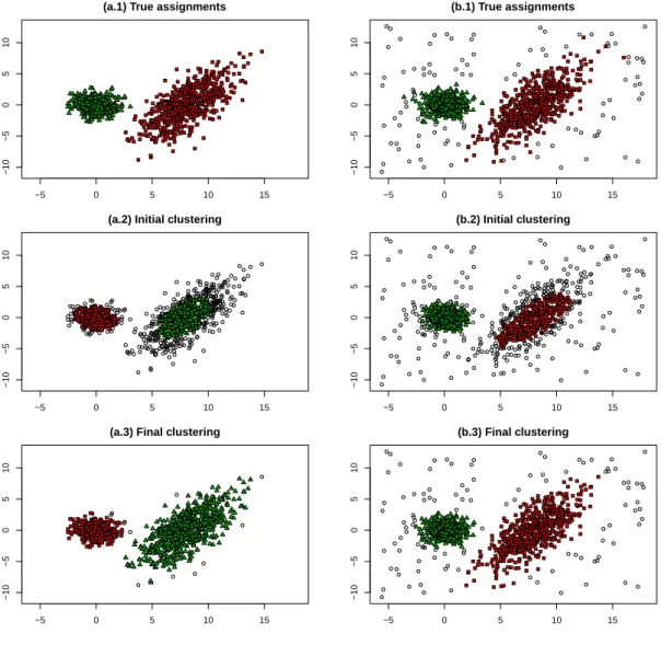
Figure 1 shows the result of applying the proposed methodology to two sim-ulated datasets. The first one shown in panel (a.1) is the result of simulating a mixture of two normal components with no contamination. In panel (b.1) 10%of the observations are replaced by outlying data points. A more detailed description of the simulation scheme will be given in Section 3. Panels (a.2) and (b.2) show the results of TCLUST (Garc´ıa-Escuderoet al., 2008) withα0 = 0.33trimming.
Several wrongly trimmed observations can be seen, but also that the TCLUST pro-cedure successfully identifies cluster cores. Finally, panels (a.3) and (b.3) show the results of the proposed methodology, which we name RTCLUST, which in both cases adapts well to the true underlying contamination.
−5 0 5 10 15
−10
−5
0
5
10
(a.1) True assignments
−5 0 5 10 15
−10
−5
0
5
10
(a.2) Initial clustering
−5 0 5 10 15
−10
−5
0
5
10
(a.3) Final clustering
−5 0 5 10 15
−10
−5
0
5
10
(b.1) True assignments
−5 0 5 10 15
−10
−5
0
5
10
(b.2) Initial clustering
−5 0 5 10 15
−10
−5
0
5
10
(b.3) Final clustering
Figure 1: Two simulated data sets with their true assignments in (a.1) and (b.1). The result of TCLUST with α0 = 0.33in (a.2) and (b.2). The final assignments
obtained after applying the proposed methodology are given in (a.3) and (b.3). Noisy data and trimmed are denoted by◦in all graphs throughout the manuscript.
spurious solutions (e.g., clusters with zero or infinite variance in some direction).It shall be underlined that the proposed reweighting methodology can be initialized from any other robust clustering method.
The underlying idea is that using an initial very robust estimator would make the procedure be resistant to a very high proportion of outliers (i.e., have a break-down point of α0). On the other hand, iteratively decreasing the trimming level
would make the procedure almost as efficient as the non-robust counterparts. A similar idea but with a different rationale was proposed in Hardin and Rocke (2004), where an initial solution is improved based on a scaled F approximation to the distribution of Mahalanobis distances (see also Hardin and Rocke (2005)). We will compare in simulations below.
It is important to stress that while we will estimate the contamination level, and evaluate masking and swamping, what we are proposing is nota method to simultaneously perform robust clustering and outlier detection. We aim at ob-taining robust and efficient estimates of partitions and model parameters. Outlier detection should then be based on robust estimators, but should be performed sep-arately based on formal rules (see e.g. Cerioli and Farcomeni (2011) for a general discussion on this point).
The outline of the paper is as follows. The proposed methodology is presented in Section 2 together with some illustrative examples and guidelines about its practical use. A simulation study is given in Section 3. Examples on a benchmark data set and on an original study on exploring the status of food security in the world are given in Section 4. Finally, Section 5 gives concluding remarks.
2
Methodology
2.1
Proposed algorithm
Let us assume that the number of clusterskis known in advance but the proportion of observationsπj in each cluster is unknown and the true contamination levelπ0
is also unknown. Non-outlying observations come from a mixture of knormally distributed components, and contamination might be present in our data. We also loosely make the assumption that the components are not too much overlapping.
We will consider a sequence of decreasing trimming levelsα0 > α1 > ... > αL withα0 being an initial preventive (i.e., surely higher than needed) trimming
level and αL is a value close to 0 that can be interpreted in a similar fashion
proportions andπl
k+1the proportion of contamination, for each trimming levelαl,
with
k+1 ∑
j=1
πjl = 1.
The center and scatter matrices estimates for the normally distributed components, in the iterationl, are denoted byµl
1, ..., µlkandΣl1, ...,Σlk.
By using this notation, the proposed methodology is described as follows:
1. Initialization:A very robust clustering is used to initialize, obtaining initial
π10, ..., πk0, π0k+1,µ10, ..., µ0kandΣ01, ...,Σ0k. We propose considering TCLUST with a high trimming levelα0 as initializing method. Letf(·;µ,Σ)denote
the p.d.f. of the p-variate normal distribution. TCLUST is based on the double maximization of
k
∑
j=1 ∑
i∈Hj
log(πjf(xi;µj,Σj)) (2.1)
with respect to parameters (µj ∈ Rp, Σj p.s.d. matrices and
∑k
j=1πj = 1)
and possible partition H0 ∪ H1 ∪ ... ∪ Hk of {x1, ..., xn}, with #H1 + ...+ #Hk = [n(1−α0)]. A proportion α0 of data is discarded in (2.1).
Maximization of (2.1) is not a well-defined mathematical problem unless spurious solutions are avoided through constraints. We use a constraint on the estimated scatter matrices is required, that is,
maxj=1,...,kmaxh=1,...,pλh(Σj)
minj=1,...,kminh=1,...,pλh(Σj)
≤c (2.2)
where {λj(Σ)}pj=1 is the set of eigenvalues of matrix Σ and c is a fixed
positive constant such that c ≥ 1. We propose using a small c value to prevent us from detecting “spurious” clusters in this initializing step. For anyα0andc, the optimal parameters solving the constrained maximization
are considered as the initialπ10, ..., πk0,µ01, ..., µ0k andΣ01, ...,Σ0k parameters. Given that we are only considering the core of the clusters, it is not possible to obtain a reliable estimation of the contamination level and, thus, we prefer just initializingπ0k+1 = 0.
maximization of (2.1) with different constraints on theΣj matrices and/or
removing the πj weights can be used. See Cuesta-Albertos et al. (1997),
Hennig (2003), Gallegos and Ritter (2005) or Neykov et al.(2007) among others. If the πj weights are removed then we may consider π10 = ... = π0
k = 1/kto initialize the procedure.
2. Reweighting process: Considerαl = α0−l·εwithε = (αL−α0)/Lfor l = 1, ..., L
2.1 Update proportions: Givenπ1l−1, ..., πkl−1, πkl−+11,µl1−1, ..., µlk−1
andΣl1−1, ...,Σlk−1from the previous step, let us consider
Di = min 1≤j≤kd
2
Σlj−1(xi, µ l−1
j ) (2.3)
and sort these values asD(1) ≤...≤D(n).Take the sets
A={xi :Di ≤D([n(1−αl)])}andB ={xi :Di ≤χ
2 p,αL}
(note that αL is used to define the set B). Now, use the distances in (2.3) to obtain a partitionA∩B ={H1, ..., Hk}with
Hj =
{
xi ∈A∩B : dΣl−1
j (xi, µ
l−1
j ) = min q=1,...,kdΣ
l−1
q (xi, µ
l−1
q )
}
.
We estimate, at this stage, the contamination level as
πkl+1 = 1− #B
n .
Ifnj = #Hj andn0 =n1+...+nk(notice thatn0is not necessarily
equal to[n(1−αl)]) then the proposed estimations at this stage of the cluster weights are
πjl = nj
n0 (
1−πlk+1). (2.4)
2.2 Update locations and scatters:We update the cluster centers by taking
µl
j equal the sample mean of the observations in Hj. To update the
scatter matrices estimates, we start fromSl
j equal to sample covariance
Additionally, covariance estimates need to be corrected by considering correcting factor defined as
cj =
(
η n0 n(1−πl
k+1)
)−1
if n0
n(1−πl k+1)
<1
and
cj = 1 if
n0 n(1−πl
k+1)
≥1
whereηβ =P
(
χ2
p+2 ≤χ2p,β
)
/βandβ = #Hj/nπj.
We finally update the scatter matrices as
Σlj =Sjl·cj.
3. Output of the algorithm: µL
1, ..., µLk andΣL1, ...,ΣLk are the final parameters
estimates for the normal components. From them, final assignments are done by computing
Di = min 1≤j≤kd
2 ΣL
j(xi, µ
L j),
fori= 1, ..., n.Observations assigned to clusterj are those inHj with
Hj =
{
xi :dΣLj(xi, µLj) = min q=1,...,kdΣ
L
q(xi, µ
L
q) andDi ≤χ2p,αL
}
and the trimmed observations are observations not assigned to any of these
Hj sets (i.e., those observations withDi > χ2p,αL).
Step 2.1 is targeted at keeping outliers outside A∩B, while increasing the trimming size in a controlled fashion. Alongside, better parameter estimates are obtained by increasing the active sample size. In the step 2.2 we use well-known correction factors (see, e.g. Liu et al., 1999) to inflate the covariance matrix esti-mates based on trimmed data. These guarantee consistency at the normal model. components. At each stage the fraction of observations in the central region of group j is nj/nπjl = n0/(n(1−πkl+1)), where nπ
l
j is an estimate of the total
number of observations in groupj.
Remark 1 More sophisticated rules for discarding outliers, for instance, based on using the Beta distribution or multiple testing corrections could have been tried (Cerioli, 2010; Cerioli and Farcomeni, 2011). However, for sake of clarity of
pre-sentation, we have preferred the simpler use of a rule just based onχ2
p,αL. There
is still room for improvement regarding better detection of outlying observations.
Remark 2 Sometimes, we could be interested in forcing some “a priori” con-straints like those in (2.2) to the final estimated clusters scatter matrices. In this case, constraints can be forced by truncating the scatter matrices eigenvalues in the updating step 2.2 as done in Fritzet al.(2013).
2.2
Illustrative examples
The two component normal mixture shown in panels (b.1) of Figure 1 account for 36% and 54% of the observations, respectively, while a 10%of not “very over-lapped” contamination is added. The scatter matrix for the first component isΣ1
equal to the identity matrix andΣ2 is a scatter matrix with|Σ2| = 20and
eigen-values equal to 11.708 and 1.708. This means that the “true” eigenvalue ratio for these two scatter matrices is equal to 11.708. A more detailed description of the process generating this data set will be given in Section 3. We will use this data set in order to illustrate the lack of dependence of the final solution on the initializing trimming levelα0and on the initial value of the restriction factorcwhen TCLUST
is used as initializing procedure. Figure 2 shows the evolution of the determinants of the scatter matrices, i.e. {|Σl
j|}Ll=0 forj = 1,2in panel (a), and the evolution
of the estimated contamination level and estimated cluster sizes, i.e. {πjl}Ll=0 for
j = 0,1,2in (b). These evolutions are studied for different values ofα0 = 0.3,
0.25, 0.2 and 0.15 and it is always considered the same (wrong) eigenvalue ratio constraint valuec= 5for the TCLUST method as initializing procedure. We can see that the final output is not very dependent on the initializing trimming level and that the output estimated parameters are very close to the true ones we want to estimate (i.e.,|Σ1|= 1and|Σ2|= 20for the cluster scatter matrices determinants
and π0 = 0.1, π1 = 0.36andπ2 = 0.54for the contamination level and cluster
sizes).
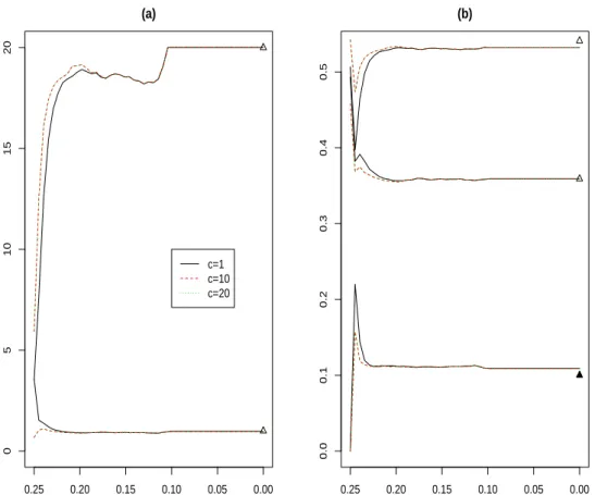
Analogously, the same type of study was made to analyze the possible depen-dence on the initializing choice ofc. The results are shown in Figure 3 where c
0.30 0.25 0.20 0.15 0.10 0.05 0.00
0
5
10
15
20
(a)
α0=0.3 α0=0.25 α0=0.2 α0=0.15
0.30 0.25 0.20 0.15 0.10 0.05 0.00
0.0
0.1
0.2
0.3
0.4
0.5
(b)
Figure 2: Evolution of |Σl
j|in (a) and of πjl in (b) for different initial α0 values
(α0 =.3, .25, .2 and .15) for the data set shown in Figure 1 (b.1). The up-triangle
symbols are the true parameters to be estimated.
are accurate and that they are not very dependent on the initialcvalue.
It is also important to note, in Figure 2 and Figure 3, that no great changes are noticeable in the estimated parameters when the procedure approximately reaches the true contamination level. This is because, we count on quite accurate esti-mators of the parameters of the normal distributions components throughout µl j
0.25 0.20 0.15 0.10 0.05 0.00
0
5
10
15
20
(a)
c=1 c=10 c=20
0.25 0.20 0.15 0.10 0.05 0.00
0.0
0.1
0.2
0.3
0.4
0.5
(b)
Figure 3: Evolution of |Σl
j| in (a) and of πjl in (b) for different initial c values
(c = 1, 10 and 20 while the true cneeded was 11.71) for the data set shown in Figure 1 (b.1). The up-triangle symbols are the true parameters to be estimated.
To reinforce our previous claims, we will illustrate the advantages of the proposed iterative trimming procedure with respect to one-step reweighting ap-proaches even in the k = 1case. When k = 1, the reweighted MCD is clearly one of the most popular robust location and scatter estimator. After considering an initial large trimming level α0, reweighting is done to increase efficiency as
described in Section 1.
Figure 4 is based in a simulated data set of size n = 1000generated from a bivariate normal distribution accounting for73% of the data (the bulk of data), a
package in Ravailable in the CRAN repository with the default initial trimming level α0 ≃ 0.5 andαL = 0.01 and the function “tolEllipsePlot” (from
“robust-base”) to plot the 0.99 tolerance ellipses (the classical and the MCD-based robust ones). Despite there exists a “good” initial sub-population including more than half of the observations, the final estimation is very distorted by the added point-wise contamination as can be seen in 4,(b). On the other hand, Figure 4,(a) shows how the proposed iterative trimming resists very well this pointwise contamina-tion.
Finally, an additional important parameter for the proposed methodology is
αL. In all the shown illustrative examples, the same αL = 0.01has been take.
The αL parameter has to do with the quantile in the χ2p distribution and it plays
the same role as in all analogous reweighting methods. For instance, αL = 0.01
means that around 1%of the observations are wrongly discarded when we have normal components without contamination. The smaller the αL the lesser is the
number of proportion of wrongly trimmed observations but higher is the risk of incorporating near outlying observations.
3
Simulation study
We now study the performance of the previously described procedure when ap-plied to several (contaminated) mixtures of Gaussian distributions. Additionally, we detail how the data sets used in previous sections have been simulated in the illustrative examples.
The non-outlying part of the dataset comes from a mixture of two p-variate normal distributionsπ1N(µ1,Σ1)+π2N(µ2,Σ2)with centersµ1 = (0,0,0, ...,0)′
andµ2 = (8,0, ...,0)′ and covariance matrices
Σ1 =Ip and Σ2 =
p
√
λ
1 1 1 1 · · · 1 1 2 2 2 · · · 2 1 2 3 3 · · · 3
..
. ... ... ... . .. ...
1 2 3 4 · · · p
.
This means that|Σ1|= 1and|Σ2|=λ.
−5 0 5 10 15 20
−5
0
5
10
15
20
(a)
−5 0 5 10 15 20
−5
0
5
10
15
20
(b)
robust classical
Figure 4: (a) The proposed iterative reweighting procedure when k = 1started fromα0 = 0and αL = 0.01(b) The (traditional) reweighted MCD started from α0 = 0andαL= 0.01. Trimmed points are the black points.
from µ1 and µ2 (using Σ1 and Σ2) smaller than χ2p,ν are discarded. The
opera-tion is repeated until the desired proporopera-tion ofεoutliers have been obtained. The parameterν controls how far away contaminated data points are.
• Three data dimensions: p= 2,4and 6
• Three contamination levelsε= 0.10, 0.05, and zero.
• Two scalesλ= 1and 5
• Balanced clustersπj = 0.5forj = 1,2and unbalanced clustersπ1 = 0.4
andπ2 = 0.6
• Twoνvalues,ν= 0.01andν = 0.005
• Two types of contamination: a symmetric one obtained sampling from a uniform distribution in the hypercube defined by the range of the non-contaminated part of the data and an asymmetric one obtained by sampling from a uniform distribution defined on[−3,0]×[−7,−2]×[−2,2]p−2, which
is closer to the second cluster than to the first.
The caseε = 0is used to evaluate efficiency of the proposed methodology when applied to clean data.
Regarding the illustrative examples in Figure 1 we generated two datasets once from a bivariate normal distribution, fixing λ = 20, π1 = 0.4 π2 = 0.6, with
symmetric contamination andν= 0.01. A contamination levelε= 0was used in (a.1) andε = 0.10in (b.1).
We compare the performance of the following robust clustering proposals:
• rtclust33 and rtclust20: The proposed iterative reweighting
ap-proach started from TCLUST with initial trimming levels α0 = 0.33and α0 = 0.2
• HR33andHR20: a one-step version of the procedure by Hardin and Rocke (2004) started from TCLUST with initial trimming levels α0 = 0.33and α0 = 0.2
• HR-it33 andHR-it20: the iterated and adapted version of Hardin and
Rocke (2004) started from TCLUST with initial trimming levelsα0 = 0.33
andα0 = 0.2
• tclust33,tclust20,tclust10andtclust05: TCLUST with fixed
The same valueαL = 0.01was used for RTCLUST and Hardin and Rocke’s
methods. For iterative procedures we fixedL= 20. The TCLUST procedure was included with with trimming levels which could be higher or the correct one. The same eigenvalue restriction factorc= 12is always applied when using TCLUST (in the initialization of RTCLUST and in the direct application of TCLUST). Note thatc= 12could be smaller or larger than the true eigenvalue ratio, depending on
pandλ.
The Hardin and Rocke’s methods are clustering algorithms based on the MCD philosophy. These methods are going to be initialized in this simulation study with exactly the same TCLUST robust clustering initial solution used for RTCLUST. Indeed Hardin and Rocke (2004) commented in their work that “any” robust clus-tering solution can be used and we have seen that TCLUST always provides quite sensible initial solutions for all the considered data sets in the simulation study. In fact, TCLUST always removes all noisy observations (together with others wrongly trimmed ones) with these high trimming levels (α0 = 0.33and 0.2). Let µ0
1, ..., µ0k,Σ01, ...,Σk0 andH00, H10, ..., Hk0 being the solution obtained by applying
the TCLUST method. The Hardin and Rocke’s approach proposes cut-off values to declare outliers based on the approximation
kj(mj −p+ 1) pmj
d2Σ0
j(xi, µ
0
j)∼Fp,mj−p+1, (3.1)
wherekj =ηβj is a correction factor (as that used in Section 2.1) with
βj = ˜hj/nj for˜hj = #Hj0
and
nj = #
{
xi :dΣl
j(xi, m
l
j) = min q=1,...,kdΣ
l
q(xi, m
l q)
}
andmj is the approximated degrees of freedom for the associated Wishart
distri-bution (see details in Hardin and Rocke (2004) and Hardin and Rocke (2005)). “HR33” and “HR20” apply directly the cut-off values in (3.1) to the observations in theH0
j sets while “HR-it33” and “HR-it20” refine theseHj0sets until
stabiliza-tion by applying the iterative steps described in Secstabiliza-tion 3.3 of Hardin and Rocke (2004).
For all the 96 different data scenarios, we generated the data 500 times and evaluated the performance of the methods in terms of:
• Mean Square Error for estimation of the mean vectorsµ1 andµ2, indicated
• Mean Square Errors associated to the logarithm of the eigenvalue ratio, indi-cated in the plots withM SEΣ. We decided to report the error associated to
this quantity since this ratio is forced in the initialization step to be smaller than a fixed constant c = 12 to avoid spurious maximizers. Nevertheless, as already commented, this is not necessarily the true eigenvalue ratio and we want to see how far the final estimated ratio is with respect the true one given that the proper estimation of the cluster scales play a key role in the detection of outliers.
• The estimated contamination levelεˆ.
• Swamping:the proportion of non outlying observations that are trimmed
• Masking:the proportion of outliers that are not trimmed
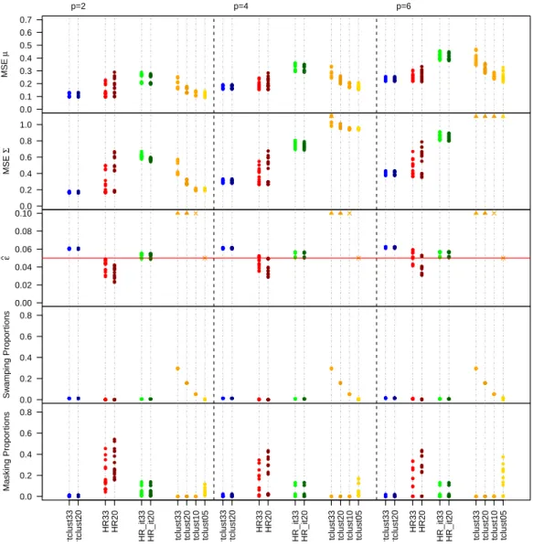
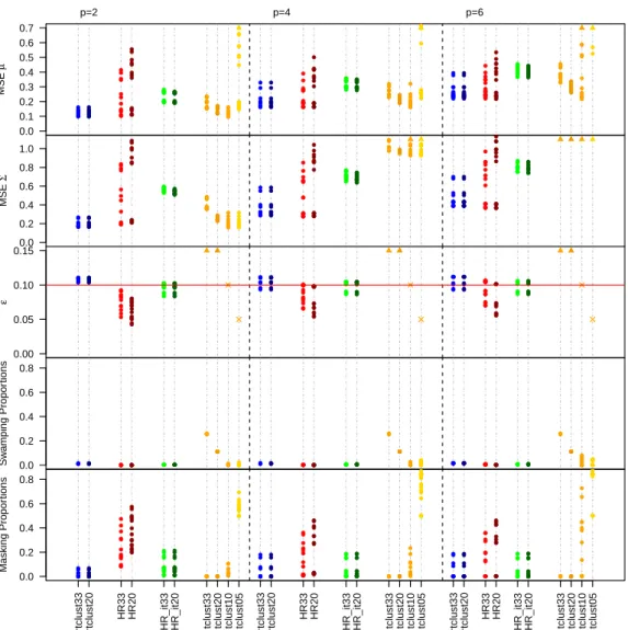
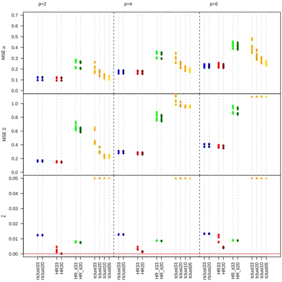
Figures 5 and 6 summarize the simulation results obtained when ε = 0.05
and0.1, respectively. Figures are separated in five row panels, one for each per-formance measure, and three column panels, one for each data dimensionality p. Given that there are several settings, in order to summarize the results in a concise way we do not distinguish among them further and just report the average perfor-mance measures all together. Note that some values exceed the scale of the plots, as identified by the upward triangle symbols.
The iterative reweighing procedure efficiently estimates the mean vector and the covariance matrix in every data scenario. In all cases we see small MSE values, and not much variability, meaning that results do not depend on the simulation set-ting considered. The MSE values are smaller than those obtained when applying TCLUST with large trimming values as 0.20 and 0.33. Moreover, MSE is even slightly better than what obtained with an oracle TCLUST whose trimming level is exactly equal to the true contamination levelε. This happens for two reasons. The first is that reweighting can adapt well to the positioning of the outliers, there-fore flexibly trimming more or less as needed within each replicate. The second is that TCLUST is based on a sometimes wrong eigenvalue ratio constraint value
c= 12. RTCLUST does not have further constraints and therefore can exceed this value when needed.
MSE
µ
0.0 0.1 0.2 0.3 0.4 0.5 0.6 0.7
p=2 p=4 p=6
MSE
Σ
0.0 0.2 0.4 0.6 0.8 1.0
ε
^
0.00 0.02 0.04 0.06 0.08 0.10
Sw
amping Propor
tions
0.0 0.2 0.4 0.6 0.8
Masking Propor
tions
0.0 0.2 0.4 0.6 0.8
rtclust33 rtclust20 HR33 HR20
HR_it33 HR_it20 tclust33 tclust20 tclust10 tclust05 rtclust33 rtclust20 HR33 HR20 HR_it33 HR_it20 tclust33 tclust20 tclust10 tclust05 rtclust33 rtclust20 HR33 HR20 HR_it33 HR_it20 tclust33 tclust20 tclust10 tclust05
Figure 5: Results whenε = 0.05. Every procedure is labeled as explained in the text. Values appearing in the Figure that are fixed in advance (e.g the trimming level for the tclustmethod) are plotted with the symbol “×” while when the considered value exceeds the scale of the plot we used a “N”
MSE
µ
0.0 0.1 0.2 0.3 0.4 0.5 0.6 0.7
p=2 p=4 p=6
MSE
Σ
0.0 0.2 0.4 0.6 0.8 1.0
ε
^
0.00 0.05 0.10 0.15
Sw
amping Propor
tions
0.0 0.2 0.4 0.6 0.8
Masking Propor
tions
0.0 0.2 0.4 0.6 0.8
rtclust33 rtclust20 HR33 HR20
HR_it33 HR_it20 tclust33 tclust20 tclust10 tclust05 rtclust33 rtclust20 HR33 HR20 HR_it33 HR_it20 tclust33 tclust20 tclust10 tclust05 rtclust33 rtclust20 HR33 HR20 HR_it33 HR_it20 tclust33 tclust20 tclust10 tclust05
Figure 6: Results whenε = 0.10. Every procedure is labeled as explained in the text.
within the correction factor, which exploits an estimator of the fraction of observa-tions in each cluster. The latter might not be resistant to outliers in our experience. We end this section by comparing the performance of these methods in the non contaminatedε= 0case. This is reported in Figure 7.
non-MSE
µ
0.0 0.1 0.2 0.3 0.4 0.5 0.6 0.7
p=2 p=4 p=6
MSE
Σ
0.0 0.2 0.4 0.6 0.8 1.0
ε
^
0.00 0.01 0.02 0.03 0.04 0.05
rtclust33 rtclust20 HR33 HR20
HR_it33 HR_it20 tclust33 tclust20 tclust10 tclust05 rtclust33 rtclust20 HR33 HR20 HR_it33 HR_it20 tclust33 tclust20 tclust10 tclust05 rtclust33 rtclust20 HR33 HR20 HR_it33 HR_it20 tclust33 tclust20 tclust10 tclust05
Figure 7: Simulation results study under no contamination (ε= 0).
4
Real data examples
4.1
Swiss Bank Notes
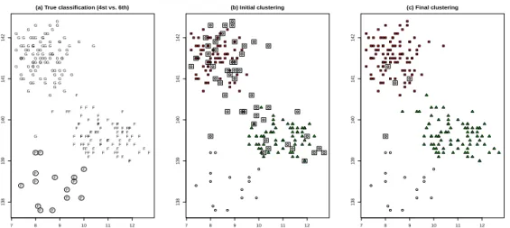
In this section we apply the proposed iterative reweighting approach to the 6 -dimensional “Swiss Bank Notes” data set presented in Flury and Riedwyl (1988) which describes certain features in 200 printed Swiss 1000-franc bank notes di-vided in two groups: 100genuine and100counterfeit notes. This is a well known benchmark data set. In Flury and Riedwyl (1988), it is pointed out that the group of forged bills is not homogeneous since 15observations arise from a different pattern and are, for that reason, outliers. Figure 8,(a) shows a scatterplot of the fourth (“Distance of the inner frame to lower border”) against the sixth variable (“Length of the diagonal”) with the classification of bills given in Flury and Ried-wyl (1988) by using symbols “G” for the genuine bills and “F” for the forged ones. The previously commented 15 “anomalous” forged bills are surrounded by circles in this graph. Figure 8,(b) shows the results of applying TCLUST with a high trimming level α0 = 0.33andc= 12. We can see that all these 15 outlying
points are successfully discarded and observations in the “cores” of the genuine and forged bills are correctly found. However, due to the use of this high trim-ming level, many observations are also discarded apart from the 15 clear outliers. We have surrounded these “probably wrongly” trimmed observations by square symbols. Finally, Figure 8,(c) shows the results of applying the proposed iterative trimming approach starting from the TCLUST’s solution in (b) withαL = 0.001.
We can see that the proportion of “probably wrongly” trimmed observations re-duces to 4 (also surrounded by square symbols). One of these 4 observations is a genuine bill which clearly exhibits certain anomalous behavior in these two plotted variables and we could also see that the other 3 (wrongly) trimmed obser-vations analogously seems to exhibit slight deviations in some of the (non-plotted) variables.
We have used a smallerαL = 0.001value in this real data example. If αL =
0.01then 7 wrongly trimmed observations (instead of 4) are obtained. As stated in the introduction, RTCLUST is not an outlier detection method. Estimates of the clusters location and scatter matrices do not change notably with the choice of
αL, which makes RTCLUST a good choice for robust clustering and parameters
estimation for this data set. Formal rules for outlier detection could be then based on RTCLUST robustly estimated parameters.
G G G G G G G G G G G G G G G G G G G G G G G G G G G G G G G G G G G G G G G G G G G G G G G G G G G G G G G G G G G G G G G G G G G G G G G G G G G G G G G G G G G G G G G G G G G G G G G G G G G G F F F F F F F F F F F F F F F F F F F F F F F F F F F F F F F F F F F F F F F F F F F F F F F F F F F F F F F F F F F F F F F F F F F F F F F F F F F F F F F F F F F F F F F F F F F F F F F F F F F F
7 8 9 10 11 12
138
139
140
141
142
(a) True classification (4st vs. 6th)
7 8 9 10 11 12
138
139
140
141
142
(b) Initial clustering
7 8 9 10 11 12
138
139
140
141
142
(c) Final clustering
Figure 8: Fourth against the sixth variable of the Swiss Bank Notes data set. (a)G
stands for genuine bills,Ffor forged ones and 15 bills listed in Flury and Riedwyl (1988) as anomalous ones are surrounded by◦symbols. (b) The initial TCLUST solution with α0 = 0.33(c) Final solution when applying the proposed iterative
approach. Trimmed observations not coinciding with those in Flury and Riedwyl’s list are surrounded bysymbols.
observations would identify them. Use of TCLUST with k = 1, ?0 = 0.5 and c = 12 (which is the default value of c fixed in the tclust package in Fritz
et al.(2012)) successfully identifies 96 genuine bills (out of the 100 non-trimmed
observations). The standard application of RTCLUST, started from this TCLUST solution with α0 = .5 andαL = 0.001, returns a final set with 102 notes which
includes 98 genuine bills. Therefore, RTCLUST is well-suited to discover, in an automatized way, the genuine observations. On the other hand, use of MCD through the well-known robustbasepackage with α = 0.5 returns 103 bills (i.e., the largest integer less than or equal to (n+p+ 1)/2 as the “best” subset found and used for computing the raw estimates. Surprisingly, only 42 out of these 103 observations are genuine ones. Additionally, things become even worse when applying the default consistency correction factor for the covariance matrix estimation and the use of (1.1) withαL = 0.025, as this finally leads to 176 notes
4.2
Food Security Data
In this section we apply the proposed procedure to an original and very recent data set on an investigation of the status of food insecurity in the world in 2014. Food security is defined by the Committee on World Food Security of United Nations as when people
at all times, have physical, social and economic access to sufficient safe and nutritious food that meets their dietary needs and food pref-erences for an active and healthy life.
For reviews see Godfrayet al.(2010) and Joneset al.(2013).
In 2014, the Gallup Organization conducted a World Poll based on a question-naire given to a representative sample of about 1000 adults from each of several areas in the world. Areas mostly correspond to countries, while in some cases countries have been split in different areas (e.g., Congo has been split in two, Brazzaville and Kinshasa areas). The Gallup World Poll (GWP) answers are then routinely summarized by Gallup into thematic indeces, which are evaluated for each polled subject and could be used to make comparisons across countries. A detailed description of the GWP can be found at
http://www.gallupworldpoll.com/content/24046/About.aspx.
In 2014 the usual GWP questionnaire has been augmented with eight questions, in partnership with the Voices of the Hungry (VoH) project of the Food and Agri-culture Organization (FAO) of the United Nations. These questions were aimed at evaluating specifically a new index, the Food Insecurity Experience Scale (FIES). A very challenging issue that has been tackled by the VoH team is the standard-ization of the FIES score over different cultures and languages. Details on how this was performed are given in Cafieroet al.(2016). A more general discussion is provided in Ballardet al.(2013); Cafieroet al.(2014).
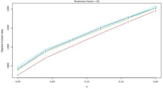
In order to explore the number of groups we use thectlcurvesof Garc´ıa-Escuderoet al.(2011), which for different values ofk show the log-likelihood at convergence of TCLUST, as a function ofαandk. They can be used to determine both the number of groups and the optimal trimming level. The ctlcurvefor the FIES data is reported in Figure 9.
0.00 0.05 0.10 0.15 0.20
−2600
−2400
−2200
−2000
CTL−Curves
α
Objectiv
e Function V
alue
Restriction Factor = 50
4
4
4
4
4
4
3
3
3
3
3
3
2
2
2
2
2
2
1
1
1
1
1
1
Figure 9: ctlcurveplot for the FIES data.
As sometimes happens, Figure 9 clearly indicates that there should bek >2
groups, but it is unclear as with respect to the choice betweenk = 3andk = 4. Additionally, it is definitely not conclusive with respect to the optimal trimming level α, which here is a parameter of interest as it is connected with the number (and identity) of outlying nations. The final estimates depend on the choice of
α. In this example, RTCLUST can be seen as an automatic way of choosing the optimal trimming level, as the one balancing between robustness and efficiency. For the proposed methodology we do not need to specifyα. We have applied our method both based on k = 3 and k = 4. As with k = 4 two groups are not very separated, we preferk = 3and report only those results for reasons of space. We run rtclustwithk = 3, initial trimming levelα0 = 0.2, αL = 0.001.The
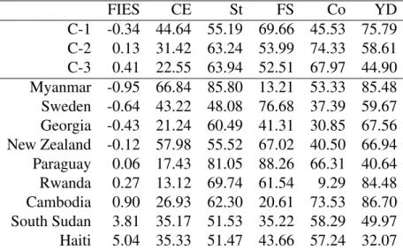
outlying countries are reported in Table 1. It shall be noted that groups 1 and 3 are of similar size as the group of outliers. Countries in groups 1 and 3 are very similar though and close to the reported profiles, while outliers are provably scattered, or have extremal values at least in one of the dimensions considered.
Table 1: Cluster profiles and measurements for the outlying countries. FIES: Food Insecurity Experience Scale. CE: Civic Engagement. St: Struggling. FS: Food Security. Co: Corruption index. YD: Youth Development. C-j:j-th cluster profile.
FIES CE St FS Co YD
C-1 -0.34 44.64 55.19 69.66 45.53 75.79 C-2 0.13 31.42 63.24 53.99 74.33 58.61 C-3 0.41 22.55 63.94 52.51 67.97 44.90 Myanmar -0.95 66.84 85.80 13.21 53.33 85.48 Sweden -0.64 43.22 48.08 76.68 37.39 59.67 Georgia -0.43 21.24 60.49 41.31 30.85 67.56 New Zealand -0.12 57.98 55.52 67.02 40.50 66.94 Paraguay 0.06 17.43 81.05 88.26 66.31 40.64 Rwanda 0.27 13.12 69.74 61.54 9.29 84.48 Cambodia 0.90 26.93 62.30 20.61 73.53 86.70 South Sudan 3.81 35.17 51.53 35.22 58.29 49.97 Haiti 5.04 35.33 51.47 43.66 57.24 32.07
It shall be noted that the new FIES score is able to separate very well the three clusters, while Gallup’s FS score only discriminates between the first and the other two. Other evidence in favor of the added value of FIES is that if we remove it and repeat the analysis the average silhouette width decreases by about 4%.
5
Conclusions and further directions
We have presented an iteratively reweighed approach that can recover wrongly trimmed observations when applying robust clustering procedures based on a high (preventive) trimming levels. This approach also makes easier the use of the TCLUST robust clustering method by diminishing its influence on the initial trimming level and on the chosen value for the eigenvalue ratio constraint. RT-CLUST has two advantages over TRT-CLUST: first, a sometimes not easily chosen tuning parameter, the trimming level, does not need to be perfectly specified in ad-vance and the same happens for the eigenvalue ratio constraint valuec. Secondly, it conjugates high robustness (as it can resist to anα0 proportion of outliers) with
high efficiency (as under no or little contamination the proportion of discarded observations will be much lower thanα0). The simulation study and the real data
example also show how this methodology could be useful in practical applica-tions. There is still room for further work. Formal theoretical properties could be explored. As commented in Remark 1, the outlier labeling process at each itera-tion could also be refined. We have applied very simple thresholds based on theχ2
among groups.
Acknowledgments
Research partially supported by the Spanish Ministerio de Econom´ıa y Compet-itividad, grant MTM2014-56235-C2-1-P, and by Consejer´ıa de Educaci´on de la Junta de Castilla y Le´on, grant VA212U13. We are grateful to Gallup, Inc. and the Voices of the Hungry project, FAO, for access to the GWP/FIES data.
References
T.J. BALLARD, A.W. KEPPLE, ANDC. CAFIERO(2013). The food insecurity experience scale: developing a global standard for monitoring hunger world-wide. Tech. rep., Food and Agriculture Organization of the United Nations, Rome.
R.W. BUTLER, P.L. DAVIES, ANDM. JHUN(1993). Asymptotics for the mini-mum covariance determinant estimator. The Annals of Statistics,21, 1385–1400.
C. CAFIERO, H. R. MELGAR-QUINONEZ, T. J. BALLARD, AND A. W. KEP -PLE(2014). Validity and reliability of food security measures.Annals of the New
York Academy of Sciences,1331, 230–248.
C. CAFIERO, M. NORD, S. VIVIANI, M. E. DEL GROSSI, T. J. BALLARD, A. W. KEPPLE, M. MILLER, ANDC. NWOSU(2016). Methods for estimating comparable rates of food insecurity experienced by adults throughout the world.
Tech. rep., Food and Agriculture Organization of the United Nations, Rome.
A. CERIOLI(2010). Multivariate outlier detection with high-breakdown estima-tors. Journal of the American Statistical Association,105, 147–156.
A. CERIOLI AND A. FARCOMENI (2011). Error rates for multivariate outlier detection. Computational Statistics and Data Analysis,55, 544–553.
A. CERIOLI, A. FARCOMENI, AND M. RIANI(2014). Strong consistency and robustness of the forward search estimator of multivariate location and scatter.
J.A. CUESTA-ALBERTOS, A. GORDALIZA, AND C. MATRAN´ (1997). Trimmedk-means: an attempt to robustify quantizers. Annals of Statistics, 25, 553–576.
A. FARCOMENI AND L. GRECO (2015). Robust Methods for Data Reduction. CRC Press.
B. FLURY AND H. RIEDWYL (1988). Multivariate Statistics. A Practical
Ap-proach. Chapman and Hall, London.
H. FRITZ, L.A. GARC´IA-ESCUDERO, AND A. MAYO-ISCAR (2012). tclust: An R package for a trimming approach to cluster analysis. J Stat Softw,47.
H. FRITZ, L.A. GARC´IA-ESCUDERO, AND A. MAYO-ISCAR (2013). A fast algorithm for robust constrained clustering. Computational Statistics and Data Analysis,61, 124–136.
M.T. GALLEGOS AND G. RITTER(2005). A robust method for cluster analysis.
Annals of Statistics,33, 347–380.
GALLUP(2015).Worldwide Research Methodology and Codebook. Gallup, Inc., Washington, D.C.
L.A. GARC´IA-ESCUDERO ANDA. GORDALIZA(2007). The importance of the scales in heterogeneous robust clustering. Computational Statistics and Data Analysis,51, 4403–4412.
L.A GARC´IA-ESCUDERO, A. GORDALIZA, C. MATRAN´ , AND A. MAYO -ISCAR (2008). A general trimming approach to robust cluster analysis. Annals
of Statistics,36, 1324–1345.
L.A GARC´IA-ESCUDERO, A. GORDALIZA, C. MATRAN´ , AND A. MAYO -ISCAR(2010). A review of robust clustering methods. Advances in Data
Analy-sis and Classification,4, 89–109.
L.A GARC´IA-ESCUDERO, A. GORDALIZA, C. MATRAN´ , AND A. MAYO -ISCAR(2011). Exploring the number of groups in robust model-based clustering.
Statistics and Computing,21, 585–599.
C. TOULMIN(2010). Food security: the challenge of feeding 9 billion people.
Science,327, 812–818.
J. HARDIN AND D.M. ROCKE(2004). Outlier detection in the multiple cluster setting using the Minimum Covariance Determinant estimator. Computational Statistics and Data Analysis,44, 625–638.
J. HARDIN AND D.M. ROCKE (2005). The distribution of robust distances.
Journal of Computational and Graphical Statistics,14.
C. HENNIG(2003). Clusters, outliers and regression: fixed point clusters.
Jour-nal of Multivariate AJour-nalysis,83, 183–212.
A.D. JONES, F.M. NGURE, G. PELTO,ANDS.L. YOUNG(2013). What are we assessing when we measure food security? A compendium and review of current metrics. Advances in Nutrition,4, 481–505.
R. Y. LIU, J. M. PARELIUS, AND K. SINGH(1999). Multivariate analysis by data depth: descriptive statistics, graphics and inference.The Annals of Statistics, 27, 783–858.
H. P. LOPUHAA (1999). Asymptotics of reweighted estimators of multivariate location and scatter. The Annals of Statistics,27, 1638–1665.
N. NEYKOV, P. FILZMOSER, R. DIMOVA, AND P. NEYTCHEV (2007). Ro-bust fitting of mixtures using the trimmed likelihood estimator. Computational Statistics and Data Analysis,52, 299–308.
M. RIANI, A. ATKINSON,ANDA. CERIOLI(2009). Finding an unknown num-ber of multivariate outliers. Journal of the Royal Statistical Society (Series B), 71, 447–466.
G. RITTER(2014). Robust cluster analysis and variable selection. CRC Press.
P. J ROUSSEEUW (1985). Multivariate estimation with high breakdown point.
Mathematical Statistics and Applications,8, 283–297.
P. J. ROUSSEEUW AND K. VAN DRIESSEN (1999). A fast algorithm for the minimum covariance determinant estimator. Technometrics,41, 212–223.
P.J. ROUSSEEUW AND A.M. LEROY (1987). Robust Regression and Outlier