Polynomial regression using a perceptron with axo-axonic connections

(1)

Polynomial Regression using a Perceptron with Axo-axonic Connections

Nuria Gómez Blas, Luis F. de Mingo, Alberto Arteta

Abstract:Social behavior is mainly based on swarm colonies, in which each individual shares its knowledge about the environment with other individuals to get optimal solutions. Such co-operative model differs from competitive models in the way that individuals die and are born by combining information of alive ones. This paper presents the particle swarm optimization with differential evolution algorithm in order to train a neural network instead the classic back propagation algorithm. The performance of a neural network for particular problems is critically dependant on the choice of the processing elements, the net architecture and the learning algorithm. This work is focused in the development of methods for the evolutionary design of artificial neural networks. This paper focuses in optimizing the topology and structure of connectivity for these networks.

Keywords: Social Intelligence, Neural Networks, Grammatical Swarm, Particle Swarm Optimization, Learning Algorithm.

ACM Classification Keywords: F.1.1 Theory of Computation Models of Computation, I.2.6 Artificial Intelligence -Learning.

Introduction

Neural networks are non-linear systems whose structure is based on principles observed in biological neuronal systems. A neural network could be seen as a system that can be able to answer a query or give an output as answer to a specific input. The in/out combination, i.e. the transfer function of the network is not programmed, but obtained through a training process on empiric datasets.

In practice the network learns the function that links input together with output by processing correct input/output couples. Actually, for each given input, within the learning process, the network gives a certain output which is not exactly the desired output, so the training algorithm modifies some parameters of the network in the desired direction. Hence, every time an example is input, the algorithm adjusts its network parameters to the optimal values for the given solution: in this way the algorithm tries to reach the best solution for all the examples. These parameters we are speaking about are essentially the weights or linking factors between each neuron that forms our network.

Neural Networks’ application fields are tipically those where classic algorithms fail because of their unflexibility (they need precise input datasets). Usually problems with unprecise input datasets are those whose number of possible input datasets is so big that they can’t be classified. For example in image recognition are used probabilistic algoithms whose efficency is lower than neural networks’ and whose caratheristics are low flexibility and high development complexity. Another field where classic algorithms are in troubles is the analisys of those phenomena whose matematical rules are unknown.

There are indeed rather complex algorithms which can analyse these phenomena but, from comparisons on the results, it comes out that neural networks result far more efficient [Hu and Hwang 2001; Katagiri 2000]: these

algorithms use Fourier’s trasform to decompose phenomena in frequential components and for this reason they

(2)

datasets just as with these systems but there is no need to restrict the problem or useFourier’s tranform. A defect common to all those methods it’s to restrict the problem setting certain hypothesis that can turn out to be wrong. We just have to train the neural network with hystorical series of data given by the phenomenon we are studying.

Calibrating a neural network means to determinate the parameters of the connections (synapsis) through the training process. Once calibrated there is need to test the netowrk efficency with known datasets, which has not been used in the learning process. There is a great number of Neural Networks which are substantially distingushed by: type of use, learning model (supervised/non-supervised), learning algorithm, architecture, etc.

This paper focuses on supervised networks with the backpropagation learning algorithm and applied to signal

analysis with a typical feedforward architecture.

Multilayer Perceptron

Multilayer perceptrons (MLPs) are layered feedforward networks [Cover and Tomas 1991] typically trained with

static backpropagation. These networks have found their way into countless applications requiring static pattern classification. Their main advantage is that they are easy to use, and that they can approximate any input-output map.

In principle, backpropagation provides a way to train networks with any number of hidden units arranged in any number of layers [Hu 1996; Hu et al. 1994]. In fact, the network does not have to be organized in layers - any pattern of connectivity that permits a partial ordering of the nodes from input to output is allowed. In other words, there must be a way to order the units such that all connections go from ”earlier" (closer to the input) to "later" ones (closer to the output). This is equivalent to stating that their connection pattern must not contain any cycles. Networks that respect this constraint are called feedforward networks; their connection pattern forms a directed acyclic graph or dag.

Backpropagation algorithm can be expressed as equation (1). Note that in order to calculate the error for unitj, we must first know the error of all its posterior nodes (forming the setPj). Again, as long as there are no cycles in the

network, there is an ordering of nodes from the output back to the input that respects this condition. For example, we can simply use the reverse of the order in which activity was propagated forward.

δj =f

0

j(netj) X

i∈Pj

δjwij (1)

Axo-axonic Neural Networks

The most usual connection type in neural networks is the axo-dendritic connection. This connection is based on the fact that the axon of an afferent neuron is connected to another neuron via a synapse on a dendrite, and modelized

inANN model by a weighted activation transfer function. But, there exists many other connection types as:

axo-somatic, axo-axonic and axo-synaptic [Delacour 1987]. This paper is focused on the second kind of connection type

axo-axonic. Merely, the structure of the axo-axonic connection can be sketched by three neurons with a classical

axo-dendritic connection and the synaptic axonal termination ofN3 connected to the synapseS12. The principle

consists on propagating the action of neuronN3as synapseS12. In order to model previous connection type, two

neural networks are required. The first (assistant) one will compute the weight matrix of the second (principal) one. And, the second network will output a response, using the previously computed weight matrix, this architecture is

(3)

ENN as Taylor series approximators.

It is well known that a function can be approximated with a given error using a polynomialP(x) = ˆf(x)with a degreen. The errorf(x)−P(x)is measure in such a way that in order to find a suitable approximation (error lower than a known threshold) it is only needed to compute sucessive derivates of functionf(x)until a certain degreen.

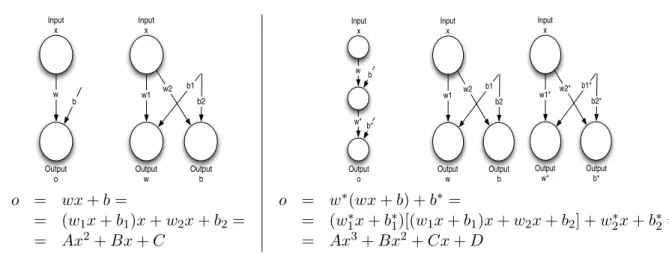
Enhanced Neural Networks behave asn-degree polynomial approximators depending on the number of hidden

layer in the architecture. In order to obtain such behavior all activation functions of the net must be lineal function

f(x) =ax+b.

w

b w1

w2 b1 b2

Output w

Output b Output

o Input

x

Input x

w1 w2 b1

b2

Output w

Output b Input

x

w1* w2* b1* b2*

Output w*

Output b* Input

x Input

x

w b

w*_b*

Output o

o = wx+b=

= (w1x+b1)x+w2x+b2=

= Ax2+Bx+C

o = w∗(wx+b) +b∗=

= (w₁∗x+b₁∗)[(w1x+b1)x+w2x+b2] +w∗2x+b∗2 =

= Ax3+Bx2+Cx+D

Figure 1: ENN architectures and output expressions

As shown in figure1and output equations, the number of hidden layers can be increased in order to increase the

degree of the output polynomial, that is, the numbernof hidden layers control, in some sense, the degreen+ 2of output polynomial of the net.

Table1shows how the degree of the output polynomial increases according to the number of hidden layers in the

net.

Table 1: Number hidden layers vs. degree of output polynomial

Hidden DegreeP(x) Output

Layers Polynomial

0 2 o=a2x2+a1x+a0

1 3 o=a3x3+a2x2+a1x+a0

· · · ·

n n+ 2 o=Pn_i₌₀+2aixi

The only condition that the learning algorithm must verified is that weights must be adjusted to values related with the sucesive derivates of functionf(x)that pattern set represents. Usually such function is unkown therefore, if the network converges with a low mean squared error then all weights of the net have converged to the derivates of functionf(x)(the pattern set unkown function), and such weights will gather some information about the function and its derivates that the pattern set represents.

Data sets

Previously defined neural network architecture has been used to approximate different data sets generated using a

(4)

Table 2: Sample of randomly generated values using an uniform distribution.

Min. 1st Qu. Median Mean 3rd Qu. Max.

-0.97600 -0.50130 0.01855 -0.04053 0.41540 0.98880

SAMPLE DATA -- Standard deviation: 0.5708282 , Variance: 0.3258449

[1] -0.05100 -0.26798 -0.77103 -0.05086 -0.26436 -0.32416 -0.96345 -0.82661 0.89400 0.86154 0.29179 0.86964 0.72917

[14] -0.38158 -0.26924 0.07974 -0.42825 0.98878 -0.87016 -0.41886 0.08352 0.25384 -0.39868 -0.97603 -0.79159 0.59038

[27] -0.96696 -0.69930 -0.95632 -0.42189 0.59004 0.65942 0.40932 -0.77566 0.16400 0.21629 0.45231 -0.39479 0.92717

[40] 0.36792 -0.49954 0.90206 0.51239 -0.72945 -0.94883 -0.97396 0.54177 0.06722 0.00008 0.59842 -0.69638 0.07971

[53] -0.50657 0.15915 0.35297 -0.73656 0.05649 0.48023 0.97079 0.17456 0.07224 0.92373 -0.64668 0.63300 -0.30577

[66] -0.16878 -0.35884 -0.15355 -0.20623 -0.97129 -0.80947 0.44842 -0.61685 0.03132 -0.41215 -0.82795 0.00578 0.98312

[79] -0.20718 -0.70245 0.27336 -0.92647 0.69454 -0.55756 0.21941 -0.03392 0.43355 0.31659 -0.21409 0.13297 0.65948

[92] -0.74168 -0.61549 0.10033 0.12152 0.06672 0.68932 -0.04284 0.04052 0.11754 0.52441 0.70085 -0.08563 0.23654

Pn= ( ¯C×X¯)2+c0, (2)

whereC¯ ={c0, c1, c2,· · ·, cn}are the coefficients andX¯ ={x1, x2,· · ·, xn}are the variables.

A neural network with no hidden layer is able to approximate such data sets with no error at all (or at least with a lower bound), according to theoretical results. Next samples presents different empirical results to justify such theoretical proposition.

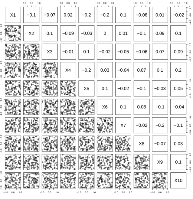
All testing data, coefficients and variable values, are generated using an uniform distribution in interval(−1,1).

Table2show some generated values and the mean, median, max, min and quartiles of such data just to check the

uniform properties of generated values. Figure2shows a correlation matrix among10variables. The table and

figure only show part of the data not all.

Polynomial regression: 2 variables

f(x, y) = (Ax+By+C)2 (3)

= A2x2+B2y2+C2+ 2ACx+ 2BCy+ 2ABxy





A2 i1 j1

i2 B2 k1

j2 k2 C2



, wherei1+i2 = 2AB, j1+j2 =−2AC, k1+k2=−2BC (4)

A neural network has been trained using a random data set with an uniform distribution and describing the polynomial function:

f(x, y) = ((x, y,1)×(−0.7909866,−0.7742045,0.726699))2 (5)

Mean squared error of the network must be equal to 0, according to the theoretical results. Next listing shows

obtained results with the proposed neural network architecture. Note that MSE in the training and cross validation data sets is really low (near0).

Number of variables: 2

Coefficients (A, B, C): -0.7909866 -0.7742045 0.726699

Squared coefficients (A*A, B*B, C*C): 0.6256597 0.5993926 0.5280914

Number of patterns: 2000 , Iterations: 102 , Learning rate: 0.05 , Cross val.: 20 %

Mean Squared Error (TRAINING):

Standard deviation 1.037659e-14 , Variance 1.076736e-28

-2.442e-14 -1.499e-14 -8.105e-15 -6.531e-15 9.159e-16 2.565e-14

(5)

X1

−1.0 0.0 1.0

−0.1 −0.07

−1.0 0.0 1.0

0.02 −0.2

−1.0 0.0 1.0

−0.2 0.1

−1.0 0.0 1.0

−0.08 0.01

−1.0 0.0 1.0

−1.0

0.0

1.0

−0.02

−1.0

0.0

1.0

X2 0.1 −0.09 −0.03 0 0.01 −0.1 0.09 0.1

X3 −0.01 0.1 −0.02 −0.05 −0.06 0.07

−1.0

0.0

1.0

0.09

−1.0

0.0

1.0

X4 −0.2 0.03 −0.04 0.07 0.1 0.2

X5 0.1 −0.02 −0.1 −0.03

−1.0

0.0

1.0

0.05

−1.0

0.0

1.0

X6 0.1 0.08 −0.1 −0.04

X7 −0.02 −0.2

−1.0

0.0

1.0

−0.1

−1.0

0.0

1.0

X8 −0.07 0.03

X9

−1.0

0.0

1.0

0.1

−1.0 0.0 1.0

−1.0

0.0

1.0

−1.0 0.0 1.0 −1.0 0.0 1.0 −1.0 0.0 1.0 −1.0 0.0 1.0

X10

(6)

Standard deviation 1.06709e-14 , Variance 1.138682e-28

-2.465e-14 -1.367e-14 -6.852e-15 -5.291e-15 2.276e-15 2.476e-14

MATRIX Network coefficients:

[,1] [,2] [,3]

[1,] 0.6256597 0.4474168 0.4502775 [2,] 0.7773538 0.5993926 0.5274104 [3,] 0.6993407 0.5978168 0.5280914

A*A = 0.6256597 , B*B = 0.5993926 , C*C = 0.5280914 2*A*B = 1.224771 , -2*A*C = 1.149618 , -2*B*C = 1.125227

Coefficients of regression polynomial can be obtained using the weights matrix of trained neural network. Previous matrix shows final weights with a cuasi-null MSE, in our case the coefficients are the following ones (according to equation4):

(A2, B2, C2) = (0.6256597,0.5993926,0.5280914) (6)

(2AB,−2AC,−2BC) = (1.224771,1.149618,1.125227) (7)

Such results are tottally coherent with equation5, that is, proposed neural network is able to approximate the data set and generate the polynomial function that describes the data set.

High dimension properties

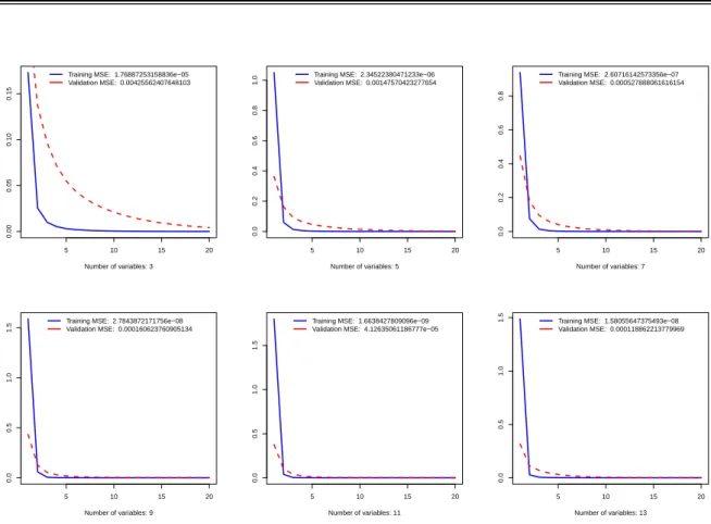
Previous neural network model behaves with the sameMSEin case using high dimension data sets. Following

listing shows the learning result of a polynomial with50variables. Table3shows a summary using different number of variables.

Coefficients (A, B, ...): -0.4198864 0.6027695 0.6039954 -0.1065414 0.9356629 0.9834093 -0.8226473 0.8743879 -0.7042015 -0.3393832 0.7709589 -0.5013933 -0.8844903 -0.699804 -0.6985472 0.5526986 0.5012762 -0.07739273 0.1085922 -0.914291 0.4816206 -0.7921206 -0.3315833 0.1244581 -0.5412277 -0.5013642 -0.9528081 0.2618788 0.2249716 -0.9169567 0.1750446 0.7072091 -0.6856862 0.3719996 -0.1491458 -0.5018547 0.9422977 0.691155 0.9959811 0.2117917 -0.1234416 0.1298864 -0.8055485 0.2700599 0.9574739 0.8468997 0.3655415 0.6998148 -0.2625522 -0.6242939 -0.9633645

Squared coefficients (A*A, B*B, ...): 0.1763046 0.3633311 0.3648104 0.01135107 0.8754651 0.9670938 0.6767485 0.7645542 0.4958998 0.115181 0.5943776 0.2513952 0.7823231 0.4897256 0.4879682

0.3054758 0.2512778 0.005989635 0.01179226 0.835928 0.2319584 0.627455 0.1099475 0.01548981 0.2929274 0.2513661 0.9078433 0.0685805 0.05061223 0.8408095 0.03064062 0.5001447 0.4701656 0.1383837 0.02224446 0.2518581 0.8879249 0.4776952 0.9919784 0.04485574 0.01523784 0.01687047 0.6489085 0.07293237 0.9167562 0.7172391 0.1336206 0.4897407 0.06893364 0.3897428 0.9280712

Number of patterns: 1850 , Iterations: 150 , Learning rate: 0.05 , Cross val.: 20 %

Mean Squared Error (TRAINING):

Standard deviation 0.08624005 , Variance 0.007437346

-0.31370 -0.03923 0.01557 0.01329 0.06721 0.28350

Mean Squared Error (CROSS VALIDATION):

Standard deviation 0.8489767 , Variance 0.7207615

-2.22700 -0.52780 0.02572 0.02860 0.57930 2.79500

MATRIX Network coefficients:

(7)

Table 3: Results with different number of variables (see figure3)

Number of patterns: 1200 , Iterations: 20 , Learning rate: 0.05 , Cross validation set: 20 %

Real coefficients: 0.885 0.814 0.114 -0.513

Squared Real coefficients: 0.783 0.663 0.013 0.263

Mean Squared Error (TRAINING): Standard deviation 0.005430024 , Variance 2.948516e-05

Min. 1st Qu. Median Mean 3rd Qu. Max. -0.0172000 -0.0030180 0.0009090 0.0006146 0.0048900 0.0106200

Mean Squared Error (CROSS VALIDATION): Stan ard deviation 0.005166362 , Variance 2.669129e-05

Min. 1st Qu. Median Mean 3rd Qu. Max. -0.0136000 -0.0026350 0.0009429 0.0006865 0.0046690 0.0107400

Network coefficients: 0.77 0.65 0.008 0.274

Real coefficients: -0.633 0.07 -0.428 -0.441 -0.858 -0.946

Squared Real coefficients: 0.401 0.005 0.183 0.194 0.736 0.895

Min. 1st Qu. Median Mean 3rd Qu. Max. -0.0047460 -0.0015840 -0.0002670 -0.0002031 0.0010550 0.0059510

Network coefficients: 0.404 0.007 0.187 0.197 0.739 0.89

Real coefficients: -0.085 0.723 -0.362 -0.662 0.049 -0.006 -0.272 -0.725

Squared Real coefficients: 0.007 0.523 0.131 0.438 0.002 0 0.074 0.525

Min. 1st Qu. Median Mean 3rd Qu. Max. -1.614e-03 -5.753e-04 -9.671e-05 -8.572e-05 3.291e-04 2.020e-03

Network coefficients: 0.008 0.524 0.131 0.439 0.003 0.001 0.075 0.523

Real coefficients: 0.601 -0.022 0.753 0.023 0.764 0.589 -0.06 -0.772 0.03 0.777

Squared Real coefficients: 0.361 0 0.567 0.001 0.584 0.347 0.004 0.596 0.001 0.604

Network coefficients: 0.361 0.001 0.567 0.001 0.584 0.347 0.004 0.596 0.001 0.603

Real coefficients: -0.915 -0.737 -0.706 -0.744 0.656 -0.332 0.981 -0.112 0.744 0.59 0.026 0.797

Squared Real coefficients: 0.837 0.543 0.498 0.553 0.43 0.11 0.962 0.013 0.554 0.348 0.001 0.636

Mean Squared Error (TRAINING): Standard deviation 4.617442e-05 , Variance 2.132077e-09

Mean Squared Error (CROSS VALIDATION): Stan ard deviation 4.979714e-05 , Variance 2.479755e-09

Network coefficients: 0.837 0.543 0.498 0.554 0.43 0.11 0.962 0.013 0.554 0.348 0.001 0.635

Real coefficients: -0.101 0.877 -0.38 -0.081 0.022 0.13 0.035 -0.428 0.076 0.364 -0.156 -0.52 0.225 -0.893

Squared Real coefficients: 0.01 0.769 0.145 0.007 0 0.017 0.001 0.183 0.006 0.133 0.024 0.271 0.05 0.798

(8)

5 10 15 20

0.00

0.05

0.10

0.15

Number of variables: 3 Training MSE: 1.76887253158836e−05 Validation MSE: 0.00425562407648103

5 10 15 20

0.0

0.2

0.4

0.6

0.8

1.0

5 10 15 20

0.0

0.2

0.4

0.6

0.8

5 10 15 20

0.0

0.5

1.0

1.5

5 10 15 20

0.0

0.5

1.0

1.5

Number of variables: 11 Training MSE: 1.6638427809096e−09 Validation MSE: 4.12635061186777e−05

5 10 15 20

0.0

0.5

1.0

1.5

Figure 3: Training and cross-validation MSE with different number of variables (see table3)

Particle Swarm Optimization and Neural Networks

Particle swarm optimization can be applied to solve many problems. One of them could be the training of a neural network architecture: Given a neural architecture, the problem is to find weights that minimize the mean squared error of the net. Individuals code weights of the neural network, and the fitness function corresponds to the mean

squared error. According to Kolmogorov a multilayer perceptron can approximate any function even when the

number of hidden neurons is unknown.

Obviously, a neural network withiinput neurons,hhidden neurons andooutput neurons it has(i+1)h+(h+1)o

weights and therefore, individuals of the PSO have(i+ 1)h+ (h+ 1)odimensions. By considering such number,

any real application with neural networks has at least20weights. A classical particle swarm algorithm could be

applied however individuals have a high dimension and then convergence depends on the random initialization.

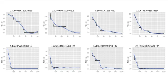
Figure 4shows the learning curve of the PSO algorithm applied to a XOR neural network. This network has a

2−2−1architecture. It can be seen that the random initialization of individuals affect the convergence process (columns of figure). And the number of iterations (100or1000, at each row) achieves a lower fitness (mean squared error). Anyway, this simple example is solved with10individuals in the population, with dimension9.

(9)

0.00590388182618566 Fitness 0.0 0.2 0.4 0.6 0.8 1.0

20 40 60 80 100

0.00409949102646106 Fitness 0.0 0.2 0.4 0.6 0.8

20 40 60 80 100

0.160407816687669 Fitness 0.2 0.4 0.6 0.8 1.0

20 40 60 80 100

0.00670879911678114 Fitness 0.0 0.2 0.4 0.6 0.8 1.0

20 40 60 80 100

4.4022377268488e−09 Fitness 0.0 0.2 0.4 0.6 0.8 1.0

200 400 600 800 1000

1.03680100831505e−22 Fitness 0.0 0.2 0.4 0.6 0.8

200 400 600 800 1000

5.28008402740878e−06 Fitness 0.0 0.2 0.4 0.6 0.8 1.0

200 400 600 800 1000

2.47236248542657e−07 Fitness 0.0 0.2 0.4 0.6 0.8 1.0

200 400 600 800 1000

Figure 4: XOR multilayer perceptron with 2 hidden neurons and a particle swarm optimization learning using 10 individuals (individuals have 9 dimensions). Each column represents a different random initialization and each row a number of iterations (100 and 1000).

Input Output

1 1 1 1 1 1 1 -1 1 1 1

1 1 1 1 1 1 -1 1 1 1 -1

1 1 1 1 1 -1 1 1 1 -1 1

1 1 1 1 -1 1 1 1 1 -1 -1

1 1 1 -1 1 1 1 1 -1 1 1

1 1 -1 1 1 1 1 1 -1 1 -1

1 -1 1 1 1 1 1 1 -1 -1 1

-1 1 1 1 1 1 1 1 -1 -1 -1

Best fitness value:5.067e-05

Best neural network weights with a8−3−3architecture:

Input layer→Hidden layer

0.1156528 1.097272 -0.946379977

-0.3683220 25.945492 -1.703378035

1.5325933 -9.765752 -0.636187430

0.4830886 26.536611 0.002121948

-1.5133460 0.790667 -0.131921926

-1.7465932 -3.369892 0.987214704

1.0519552 -4.920479 0.005404300

0.3397246 -1.924014 3.273439670

Bias: 0.7092471 -5.304714 -0.331283300

Hidden layer→Output layer

1.261584 -4.759320 0.9853185

148.541038 -1.054461 -3.1161444

-162.388447 -2.017318 -3.4691962

Bias: 0.090192 1.207254 1.9260548

These two neural examples have shown that theP SOcan be successfully applied to the particle swarm algorithm

(10)

0.448928449507574 100 Fitness 0.5 0.6 0.7 0.8 0.9 1.0

20 40 60 80 100

0.380432955845818 200 Fitness 0.4 0.5 0.6 0.7 0.8 0.9 1.0

50 100 150 200

0.166155810190459 300 Fitness 0.2 0.4 0.6 0.8 1.0

50 100 150 200 250 300

0.0857910229358835 400 Fitness 0.2 0.4 0.6 0.8 1.0

100 200 300 400

0.254269716684872 100 Fitness 0.3 0.4 0.5 0.6 0.7 0.8 0.9

20 40 60 80 100

0.0718653921693906 200 Fitness 0.2 0.4 0.6 0.8 1.0

50 100 150 200

0.0865752460809145 300 Fitness 0.2 0.4 0.6 0.8

50 100 150 200 250 300

0.000314184787007479 400 Fitness 0.0 0.2 0.4 0.6 0.8

100 200 300 400

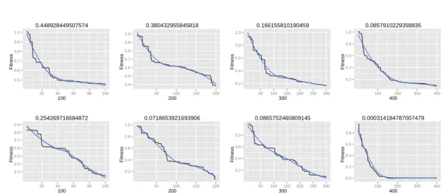
Figure 5: Binary coding neural network form8 inputs to3outputs. First row is a neural network with 3hidden

neurons and second row a neural network with 5 hidden neurons. Mean squared error (fitness of the PSO)

decreases as the number of iterations (100to400) increases.

The XOR example with dimension9and the binary-coding example with dimension39are a good starting point to

combined classical neural networks with swarm intelligence.

Conclusion

The problem of nonlinear constrained optimization arises frequently in engineering. In general it does not have a deterministic solution. In the past, nonlinear optimization methods were developed and now it is a challenge to work with differentiable functions. Before gradient methods were used successfully for solving some problems. Evolutionary methods provide a new possibility for solving such problems. The PSO technique has been used successfully in optimizing real functions without restrictions, but it has been little used for problems with restrictions.

This has happened mainly because there are no mechanism to incorporate restrictions on the fitness function.

Evolutionary Computation has tried to solve the constrained optimization problem, either by bypassing nonfeasible solutions sequences, or by using a penalty function for nonfeasible sequences. Some researchers suggest to use

two subfunctions offitness. One helps to evaluate feasible elements and the other one evaluates the unfeasible

one. In this regard, there are many criteria. Moreover, some special self adaptive functions have been designed to implement the penalty technique.

Hu and Eberhart [Hu and Eberhart 2002] presented a PSO algorithm. This algorithm bypasses nonfeasible sequences. it also creates a random initial population, in which nonfeasible sequences are bypassed until the entire population has only feasible particles. By upgrading the positions of the particles nonfeasible sequences are bypassed automatically. The cost of the technique that creates the initial populations is high; especially when it comes to problems with nonlinear constraints because then it must create an entire population of feasible individuals. In his work, Cagnina et al [Cagnina et al. 2008] proposed the following strategies for implementing the PSO into problems with restrictions: a)If two particles are feasible, select the one with the bestfitness. b)When a particle is feasible and the other is not, the feasible one is chosen. c)If two particles are nonfeasible, the one with the lowest degree of nonfeasibility is selected. These strategies are applied when the particlesgbestandlbestare selected.

We propose to analyze the penalty methods under E.A. perspective (Evolutionary Algorithms). The penalty methods use functions (penalty functions) that degrade the quality of the nonfeasible solution. In this way the constrained problem becomes a problem without constraints by using a modified evaluation function:

eval(x) =

f(x) x∈ F

(11)

F is the set created by the intersection of all sets that are the restrictions of the problem (Feasible region). The penalty is zero if no violation occurs and it is positive otherwise. The penalty function is based on the distance

between a nonfeasible sequence and the feasible region F, It also works for repairing solutions outside of the

feasible regionF.

Acknowledgements

The research was supported by the Spanish Research Agency projects TRA2010-15645 and TEC2010-21303-C04-02.

Appendix A: Implementation in R

t r a i n < - f u n c t i o n ( iter , alpha , p a t r o n e s _ in , p a t r o n e s _ out , test , v e r b o s e ) { p a t r o n e s _ in < - as . m a t r i x ( p a t r o n e s _ in )

p a t r o n e s _ out < - as . m a t r i x ( p a t r o n e s _ out ) e n t r a d a s < - n c o l ( p a t r o n e s _ in )

s a l i d a s < - l e n g t h ( p a t r o n e s _ out [1 ,])

num _ p a t r o n e s < - r o u n d ( n r o w ( p a t r o n e s _ in ) * (1 - t e s t ) , d i g i t s =0) num _ p a t r o n e s _ t e s t < - n r o w ( p a t r o n e s _ in )

num _ p e s o s < - ( e n t r a d a s +1) * s a l i d a s

m a t r i z _ p e s o s _ a u x i l i a r < - m a t r i x ( r u n i f (( e n t r a d a s +1) * num _ p e s o s ) , n r o w =( e n t r a d a s +1) , n c o l = num _ p e s o s ) m a t r i z _ p e s o s _ p r i n c i p a l < - m a t r i x ( r u n i f (( e n t r a d a s +1) * s a l i d a s ) , n r o w =( e n t r a d a s +1) , n c o l = s a l i d a s ) mse < - (1: i t e r )

mse _ t e s t < - (1: i t e r ) for ( i in 1: i t e r ) {

mse [ i ] < - 0.0

for ( id _ p a t r o n in 1: num _ p a t r o n e s ) {

p a t r o n _ in < - c (( p a t r o n e s _ in [ id _ patron ,]) , -1) p a t r o n _ out < - c (( p a t r o n e s _ out [ id _ patron , ] ) )

s a l i d a _ red _ a u x i l i a r < - p a t r o n _ in % * % m a t r i z _ p e s o s _ a u x i l i a r

m a t r i z _ p e s o s _ p r i n c i p a l < - ( m a t r i x ( s a l i d a _ red _ a u x i l i a r , n r o w =( e n t r a d a s +1) , n c o l = s a l i d a s )) s a l i d a _ red _ p r i n c i p a l < - p a t r o n _ in % * % m a t r i z _ p e s o s _ p r i n c i p a l

e r r o r < - ( s a l i d a _ red _ p r i n c i p a l - p a t r o n _ out ) mse [ i ] < - mse [ i ] + sum ( e r r o r * e r r o r * 0 . 5 )

v a r i a c i o n _ p e s o s < - - a l p h a * ( e r r o r )

m a t r i z _ p e s o s _ p r i n c i p a l < - m a t r i z _ p e s o s _ p r i n c i p a l + t ( m a t r i x ( v a r i a c i o n _ pesos , n r o w =( s a l i d a s ) , n c o l =( e n t r a d a s + 1 ) ) ) * ( m a t r i x ( p a t r o n _ in , e n t r a d a s +1 , s a l i d a s ))

v e c t o r _ s a l i d a _ red _ a u x i l i a r < - c (( m a t r i z _ p e s o s _ p r i n c i p a l ))

e r r o r _ a u x i l i a r < - ( s a l i d a _ red _ a u x i l i a r - v e c t o r _ s a l i d a _ red _ a u x i l i a r )

v a r i a c i o n _ p e s o s _ a u x i l i a r < - - a l p h a * e r r o r _ a u x i l i a r

m a t r i z _ p e s o s _ a u x i l i a r < - m a t r i z _ p e s o s _ a u x i l i a r + t ( m a t r i x ( v a r i a c i o n _ p e s o s _ a u x i l i a r , n r o w =( num _ p e s o s ) , n c o l =( e n t r a d a s + 1 ) ) ) * ( m a t r i x ( p a t r o n _ in , e n t r a d a s +1 , num _ p e s o s ))

}

s a l i d a _ t e s t < - t e s t ( m a t r i z _ p e s o s _ a u x i l i a r , p a t r o n e s _ in [( num _ p a t r o n e s + 1 ) : num _ p a t r o n e s _ test , ] , ( p a t r o n e s _ out [( num _ p a t r o n e s + 1 ) : num _ p a t r o n e s _ test , ]))

mse _ t e s t [ i ] < - ( sum ( abs ( s a l i d a _ t e s t - ( p a t r o n e s _ out [( num _ p a t r o n e s + 1 ) : num _ p a t r o n e s _ test , ] ) ) ) / ( num _ p a t r o n e s _ test - num _ p a t r o n e s )) / s a l i d a s

if (( verbose >0) & & ( i %% v e r b o s e ) = = 0 ) {

cat ( " I t e r a t i o n " , i , " - - > MSE " ,( mse [ i ] / num _ p a t r o n e s ) / salidas , " \ t \ t - - > CV " , mse _ t e s t [ i ] , " \ n " ) }

mse [ i ] < - ( mse [ i ] / num _ p a t r o n e s ) / s a l i d a s }

t r a i n < - l i s t ( mpa = m a t r i z _ p e s o s _ a u x i l i a r , mse = mse , mse _ t e s t = mse _ t e s t ) }

t e s t < - f u n c t i o n ( m a t r i z _ p e s o s _ a u x i l i a r , p a t r o n e s _ in , p a t r o n e s _ out ) {

p a t r o n e s _ in < - as . m a t r i x ( p a t r o n e s _ in ) p a t r o n e s _ out < - as . m a t r i x ( p a t r o n e s _ out ) e n t r a d a s < - n c o l ( p a t r o n e s _ in )

s a l i d a s < - l e n g t h ( p a t r o n e s _ out [1 ,]) num _ p a t r o n e s < - n r o w ( p a t r o n e s _ in ) num _ p e s o s < - ( e n t r a d a s +1) * s a l i d a s s a l i d a _ red < - p a t r o n e s _ out

for ( id _ p a t r o n in 1: num _ p a t r o n e s ) {

p a t r o n _ in < - c (( p a t r o n e s _ in [ id _ patron ,]) , -1)

s a l i d a _ red _ a u x i l i a r < - p a t r o n _ in % * % m a t r i z _ p e s o s _ a u x i l i a r

m a t r i z _ p e s o s _ p r i n c i p a l < - ( m a t r i x ( s a l i d a _ red _ a u x i l i a r , n r o w =( e n t r a d a s +1) , n c o l = s a l i d a s )) s a l i d a _ red _ p r i n c i p a l < - p a t r o n _ in % * % m a t r i z _ p e s o s _ p r i n c i p a l

s a l i d a _ red [ id _ patron ,] < - ( s a l i d a _ red _ p r i n c i p a l ) }

t e s t < - s a l i d a _ red }

(12)

{

par ( usr = c (0 , 1 , 0 , 1))

txt < - as . c h a r a c t e r ( f o r m a t ( cor ( x , y ) , d i g i t s = 2 ) ) t e x t (0.5 , 0.5 , txt , cex = 1.5 * ( abs ( cor ( x , y ))) + 2 ) }

p l o t _ c o r r e l a t i o n < - f u n c t i o n ( p a t r o n e s _ in , p a t r o n e s _ out , n e t w o r k _ o u t p u t ) {

p a i r s ( d a t a . f r a m e ( p a t r o n e s _ in , p a t r o n e s _ out , n e t w o r k _ o u t p u t ) , u p p e r . p a n e l = p a n e l . cor , m a i n = " R e l a t i o n s h i p s b e t w e e n c h a r a c t e r i s t i c s of d a t a " , col = " g r a y " , cex = 0 . 5 ) }

p l o t _ mse < - f u n c t i o n ( mpa , t i t l e = " " , x l a b e l = " " , y l a b e l = " " ) { i t e r a c i o n e s < - l e n g t h ( mpa $ mse )

p l o t ( c (1: i t e r a c i o n e s ) , mpa $ mse , lty =1 , t y p e = " l " , m a i n = c ( t i t l e ) , x l a b = xlabel , y l a b = ylabel , col = " b l u e " , lwd =2) l i n e s ( c (1: i t e r a c i o n e s ) , mpa $ mse _ test , lty =2 , col = " red " , lwd =2)

l e g e n d ( " top " , bty = " n " , cex =1 , l e g e n d = c ( p a s t e ( " T r a i n i n g MSE : " , mpa $ mse [ i t e r a c i o n e s ]) , p a s t e ( " V a l i d a t i o n MSE : " , mpa $ mse _ t e s t [ i t e r a c i o n e s ])) , col = c ( " b l u e " , " red " ) , lty =1 , lwd =2) }

Bibliography

Cagnina, L. C., Esquivel, S. C., and Coello, C. (2008). Solving engineering optimization problems with the simpel constrained particle swarm optimizer.Informatica, 32:319–326.

Cover, T. M. and Tomas, J. A. (1991). Elements of information theory. John Willey Sons.

Delacour, J. (1987). Apprentissage et memoire: Une approache neurobiologique. Masson.

Hu, X. and Eberhart, R. (2002). Solving constrained nonlinear optimization problems with particle swarm

optimization. In6th world Multiconference on Systemics, Cybernetics and Informatics., volume 5.

Hu, Y. H. (1996). Pattern classification with multiple classifiers. Technical report, Department of Electrical Computing Engineering. University of Wisconsin, Madison.

Hu, Y. H. and Hwang, J.-N. (2001).Handbook of neural network signal processing VE profiling. CRC Press.

Hu, Y. H., Tompkins, W. J., Urrusti, J. L., and Afonso, V. X. (1994). Applications of artificial neural networks for ecg.

Journal of electrocardiology, 26:66–73.

Katagiri, S. (2000). Handbook of neural networks for speech processing. Artech House.

Authors’ Information

Nuria Gómez Blas- Dept. Organización y Estructura de la Información, Escuela Univesitaria de Informática, Universidad Politécnica de Madrid, Crta. de Valencia km. 7, 28031 Madrid, Spain; e-mail:[email protected]

Major Fields of Scientific Research: Bio-inspired Algorithms, Natural Computing

Luis Fernando de Mingo López- Dept. Organización y Estructura de la Información, Escuela Univesitaria de Informática, Universidad Politécnica de Madrid, Crta. de Valencia km. 7, 28031 Madrid, Spain; e-mail:[email protected]

Major Fields of Scientific Research: Artificial Intelligence, Social Intelligence

Alberto Arteta - Dept. Tecnología Fotónica, ETSI Telecomunicación, Universidad Politécnica de Madrid, Avenida Complutense 30, Ciudad Universitaria, 28040 Madrid, Spain; e-mail:

[email protected]