Evolution and breakup of viscous rotating drops
M. A. Fontelos
1, V. J. Garc´ıa-Garrido
1, and U. Kindel´
an
21Instituto de Ciencias Matem´aticas (CSIC - UAM - UC3M - UCM). C/Nicol´as Cabrera, 13-15, Campus de
Cantoblanco, 28049 Madrid, Spain. Email: [email protected] , [email protected]. 2
Departamento de Matem´atica Aplicada y Met. Inf., Universidad Polit´ecnica de Madrid, Alenza 4, 28003 Madrid, Spain. Email: [email protected].
August 18, 2011
Abstract
We study the evolution of a viscous fluid drop rotating about a fixed axis at constant angular velocity Ω or constant angular momentumLsurrounded by another viscous fluid. The problem is considered in the limit of large Ekman number and small Reynolds number. The analysis is carried out by combining asymptotic analysis and full numerical simulation by means of the boundary element method. We pay special attention to the stability/instability of equilibrium shapes and the possible formation of singularities representing a change in the topology of the fluid domain. When the evolution is at constant Ω, depending on its value, drops can take the form of a flat film whose thickness goes to zero in finite time or an elongated filament that extends indefinitely. When evolution takes place at constant L, and axial symmetry is imposed, thin films surrounded by a toroidal rim can develop, but the film thickness does not vanish in finite time. When axial symmetry is not imposed and Lis sufficiently large, drops break axial symmetry and, depending on the value of L, reach an equilibrium configuration with a 2-fold symmetry or break up into several drops with a 2 or 3-fold symmetry. The mechanism of breakup is also described.
Keywords: Rotating drops at low Reynolds number, boundary element method, drop breakup, self-similarity and singularities.
1
Introduction
In many processes one has to deal with rotating masses of fluid. This is the case of industrial applications such as polymer manufacturing [20] and spinning drop tensiometry techniques used to measure surface and interfacial tension [24]. At atomic level, a model for nuclear fission as the breakup of a charged rotating liquid drop, where nuclear forces play the role of surface tension, was proposed by Bohr & Wheele in 1939 [4]. On astronomical scales, shapes and stability of self-gravitating masses rotating freely in space were studied in detail by Chandrasekhar [7].
Studies concerning the evolution of rotating drops date back to the original experiments of J. Plateau [21]. In those experiments, an oil drop was immersed in a tank containing a mixture of water and alcohol with almost the same density as oil. By inserting a shaft through the drop and turning it, rotation on the drop was achieved. Plateau then observed how the drop evolved through a sequence of different shapes as the angular speed was increased. In recent years, experiments aimed in the same direction as the ones performed by Plateau in 1843 have been conducted under zero gravity conditions during the flight of Spacelab 3 and at JPL (Jet Propulsion Laboratory). For a fully detailed description on these experiments see for instance [29] and [30].
Although there is a huge wealth of equilibrium shapes, one cannot expect that all of them come up to be stable. Once a rotating drop in equilibrium destabilizes, there are essentially two possibilities: the drop may undergo a transition towards another equilibrium shape, or evolve in such a way that its surface becomes non-smooth at some time and a singularity, whether representing a surface cusp or a topological change in the drop (via break up into smaller drops, for instance), develops. The fact that singularities may take place in free-surface hydrodynamic flows is well known and has been the subject of intensive research in various contexts such as capillary drop breakup or air entrainment (see [10] for an updated general review on free-surface flows and [11] for a review on singularities in general).
In order to compute the evolution of a viscous drop under rotation, one must solve the Navier-Stokes equations both inside the drop and in the fluid surrounding it, subject to suitable boundary conditions. If the Reynolds number is small, then inertial terms can be neglected in comparison with both viscous forces and centrifugal forces and one arrives then to Stokes system subject to centrifugal forces. This is the approach adopted by Howell et al. [15] to study the evolution and possible singularity formation of an axisymmetric drop rotating with constant angular velocity. Under a thin film approximation, Howell et al. show that for sufficiently large angular velocities, drops may become very flat and thin at the center with a torus-like boundary (apizza shape, in the notation of [15]). Moreover, they find that the thickness of the center can become zero in finite time so that a hole develops.
When dealing with the evolution of a fluid at small Reynolds number the approximation by Stokes system is justified. In this case, the fluid dynamics equations become linear and one can write the problem in the form of the so-called boundary integral formulation (cf. [23]). This is very suitable for numerical simulation since it allows to compute the velocity field at the boundary of the drop, and hence the evolution of the drop’s shape, by evaluating integrals restricted to the boundary itself (see [23] or [5], for instance). The boundary integral formulation is particularly interesting when dealing with the possible formation of singularities, like those appearing in the evolution of charged droplets [3], [12].
In this article we implement a boundary element method to compute the evolution of drops rotating around a fixed axis, determine the stability/instability of equilibrium shapes and study the formation of singularities that give rise to topological changes in the drop. In Section 2 we introduce the system of equations that we are going to solve. In Section 3, the details of the numerical method used are explained. Since we aim to analyze singularities that develop at the drop’s surface, special attention must be paid to local refinement and regularization of the mesh. In Section 4 we study the evolution of axisymmetric drops. Section 5 will be devoted to the study of general 3D drops both at constant angular velocity and constant angular momentum. Finally, in Section 6 we summarize the conclusions of our work.
2
Equations
Consider two viscous incompressible fluids: one for the drop and another for its surrounding media. The fluid drop has viscosity µ1 and density ρ1, while the surrounding fluid has viscosityµ2 and densityρ2. We denote the velocity and pressure of the fluid inside the drop byu(1)andp(1)respectively and the velocity and pressure
of the outer fluid by u(2) and p(2) respectively. Both fluids are rotating around a common axis with angular
velocity ω. In this situation, one can take a system of reference that is rotating with the fluids (non-inertial frame) and therefore introduce inertial forces in the Navier-Stokes equations so that
ρi (
u(ti)+u(i)· ∇u(i)
)
= −∇p(i)+µi∆u(i)−2ρiω×u(i)−ρiω×(ω×r) inDi(t) , (1)
∇ ·u(i) = 0 inDi(t) , (2)
where D1(t) is the domain enclosed by the fluid drop andD2(t) is the domain of the surrounding fluid. The third and fourth terms on the right-hand side of (1) are called Coriolis force and centrifugal force respectively. As boundary conditions, we impose balance of stresses across the interface of both fluids
(
T(2)−T(1) )
n= 2γκn on∂D(t) , (3)
whereκis the mean curvature of the interface, i.e. the average of principal curvatures,γis the surface tension, andT(k) is the stress tensor inside (k= 1) and outside (k= 2) the drop, given by:
Tij(k)=−p(k)δij+µk
( ∂u(ik)
∂xj
+∂u
(k)
j
∂xi
)
Equation (3) expresses the balance between viscous stresses and capillary forces at the interface. The normal component of the velocity has to be continuous across the boundary
u(1)·n=u(2)·n≡u·n,
wherenis the unit normal to∂D(t) pointing outward from the fluid drop. The kinematic condition is
vN =u·n on∂D(t) , (5)
vN being the normal velocity of the free boundary∂D(t).
If the axis of rotation is fixed, then
ω×(ω×r) =−ω2rer,
whereω =|ω|is the angular speed, ris the distance of the point located atrto the axis of rotation and er is
the polar radial vector. Notice that the centrifugal force−ρiω×(ω×r) is then directed in the outward radial direction. It is useful to write the centrifugal force in the form
ρiω2rer=∇ (
1 2ρiω
2r2 )
,
since the centrifugal force is conservative, and define
Π(i)=p(i)−1
2ρiω
2r2,
as the reduced pressure. Then, system (1)-(2) becomes
ρi
(
u(ti)+u(i)· ∇u(i)
)
= −∇Π(i)+µi∆u(i)−2ρiω×u(i) in Di(t) , (6)
∇ ·u(i) = 0 inDi(t) , (7)
and boundary condition (3) can be written as
(
T(2)−T(1) )
n=
(
2γκ+(ρ2−ρ1)
2 ω
2r2 )
n on∂D(t) , (8)
where we take now the following definition forT(k):
Tij(k)=−Π(k)δij+µk
( ∂u(ik)
∂xj
+∂u
(k)
j
∂xi
)
, k= 1,2,
instead of (4). In order to non-dimensionalize the system (6)-(7) we introduce a characteristic lengthl (of the order of the radius of the drop), a typical velocityU (ωl, for instance) and a characteristic time scaleτ=l/U. We will also suppose without loss of generality that the axis of rotation is the z axis. Taking µ and ρto be reference values for the viscosity and density of the fluids respectively (we can take them as those of the drop) and defining the new variables:
u(i)= u
(i)
U , r=
r
l , t= t τ , Π
(i)
= l
µUΠ
(i) , ω=ωbz , µ
i=
µi
µ , ρi= ρi
ρ ,
we get, omitting overbars to simplify notation, the non-dimensional problem:
ρiRe (
u(ti)+u(i)· ∇u(i)
)
= −∇Π(i)+µi∆u(i)− 2
Ekbz×u
(i) in D
i(t) , (9)
∇ ·u(i) = 0 inDi(t) .
Two dimensionless parameters arise: Re is the Reynolds number (measures the relative importance between inertial and viscous forces) and Ek is the Ekman number (characterizing the relation between Coriolis and viscous forces). They are defined as:
Re=ρU l
To complete the non-dimensionalization process one has to scale the boundary condition. If we define:
κ=lκ , r= r
l , T
(k)
= l
µUT
(k),
then (8) can be written as:
(
T(2)−T(1) )
n= 1
Ca (
2κ−Bo
2 r
2 )
n on∂D(t) , (10)
where overbars are omitted as before. Two new dimensionless parameters come into play, Ca andBo, called capillary number and rotational Bond number respectively:
Ca= µU
γ , Bo=
(ρ1−ρ2)ω2l3
γ .
The first one measures the relative importance of viscous to capillary forces and the second one the importance of centrifugal forces relative to capillary forces. We take as a characteristic length scale of the problem, for instance, l = √3V ol, with V ol being the volume of the drop, and a dimensionless angular velocity defined as Ω =√Bo to describe our results. Dealing with the limit in whichRe≪1 andEk≫1 , so that viscous forces dominate over inertial and Coriolis forces, we can approximate Navier-Stokes equations by the Stokes system:
−∇Π(i)+µi∆u(i) = 0 inDi(t) , (11)
∇ ·u(i) = 0 inDi(t) , (12)
which is numerically solved in the next section using the boundary element method. Since (11)-(12) together with the boundary condition (10) form a linear system, one can remove de dependence onCaby simply rescaling again the unknownsu(i), Π(i). Therefore, we will consider without loss of generalityCa= 1.
Concerning the stationary problem (where u(i)≡0), equilibrium solutions can be calculated by solving the
following differential equation:
2κ=−Π +Bo 2 r
2 on∂D, (13)
where Π = Π2−Π1 is the pressure difference sustained across the interface of both fluids. It is interesting
to point out that this differential equation for equilibrium shapes can be obtained by invoking a variational argument (cf. [7], [6]). In this variational approach, an energy functional defined by taking into account the surface energy and the rotational kinetic energy of the drop is minimized subject to a volume preservation constraint. The energy to be minimized is defined in two different ways depending on the kind of problem considered. If we have a drop rotating with constant angular speed Ω, then the energy of the system is:
E=A−1
2IΩ
2, (14)
whereAis the area of the surface ∂DandI is the moment of inertia of the drop, defined by the formula:
I=
∫
D
r2dV , (15)
withrbeing the distance from a point located atr∈ Dto the axis of rotation. On the other hand, if the drop is mechanically isolated (angular momentum is constant), the energy functional is given by:
E=A+1 2IΩ
2=A+L2
2I , (16)
whereL=IΩ is the angular momentum of the fluid drop. Finally, we remark that our non-dimensionalization is slightly different from [6], since we aimed to obtain the expressions (14) and (16) that we believe are physically more intuitive. There is a simple relation between our values of (Ω, L) and those of [6], denoted by (ΩBS, LBS):
(Ω, L) =
(
4
√ 2π
3ΩBS,8
√
2(43π)7/6LBS
)
3
Numerical method
Our interest in the evolution of the drop’s surface suggests the use of the boundary element method (BEM) to calculate the velocity at the interface between the two fluids. The BEM we have implemented is based on the boundary integral formulation of the Stokes system (11) with the boundary condition (10) (see [23], [25] for a comprehensive explanation). According to this, the equation for the velocity at∂D(t) can be written as
uj(rp) = −
1 4π
1
µ1+µ2 ∫
∂D(t)
fi(r)Gij(r,rp)dS(r)
− 1
4π
µ1−µ2 µ2+µ1
∫
∂D(t)
ui(r)Tijk(r,rp)nk(r)dS(r), i, j, k= 1,2,3, (17)
whererp is the position vector of a pointpof the surface, and
Gij(r,rp) =
δij
|r−rp|+
(ri−rp,i)(rj−rp,j)
|r−rp|3 , i, j, k= 1,2,3, (18)
Tijk(r,rp) = −6
(ri−rp,i)(rj−rp,j)(rk−rp,k)
|r−rp|5 , i, j, k= 1,2,3, (19)
fi(r) =
[
2κ(r)−1 2Ω
2r2 ]
ni(r), i= 1,2,3. (20)
At any given time t > 0, we approximate the free boundary ∂D(t) with a triangular mesh. The mesh is made up ofN vertices andM (triangular) faces. On each node, we approximate the various physical quantities that are defined on the surface (centrifugal force, curvature, velocity) with elementwise constant functions over a “virtual” element centered in each node with an area equal to one third of the total area of the elements that share the node (see [31]). We also use the nodes of the mesh as collocation points.
The general description of how we solve the integral equations is as follows: first we calculate the curvature
κin each node of the mesh, second we calculate the velocity by obtaining the balance force term f from the centrifugal force and κ, replacing it in (17) and solving the resulting integral equation. Given the velocity
u, we move the points of the surface using the explicit Euler scheme and regularize the mesh. In the next subsections we will describe the BEM used to compute the velocity field at the surface of the drop (including the regularization and refinement of the mesh) and the two procedures we have implemented for computing the mean curvature of the drop’s surface and the moment of inertia of the drop. We have used two codes based on the general principles sketched above. In the simplest one, axial symmetry is assumed and explicit integration of the boundary integral in the polar coordinateθ is performed. The other code does not assume any kind of symmetry and is the one we explain in more detail in this section. The axisymmetric code is a simplified version of it and so we briefly describe it at the end of the section.
3.1
Mean curvature
We calculate the mean curvature in each nodepof the mesh following a method proposed in [31]. The algorithm is based on the following idea. If thez′ axis of the local cartesian coordinates (rp, x′, y′, z′) was directed along
the normal vectornp, then z′ as a quadratic function ofx′ andy′ would be a good local representation of the surface ∂D. This quadratic function can be obtained by finding a paraboloid which passes throughp, has its axis parallel toz′ and fits best its neighbors by the least-squares method. Howevernp is not knowna priori, and so the method is iterative. The formal description of this method appears in algorithm 1.
Note that due to the use of the least-squares method, each node of the mesh must have 5 or more neighbors. The convergence is very fast with only a few iterations needed, even for ε ∼10−6−10−8. We also use this algorithm to calculate the normal vector to the surface at each node of the mesh.
3.2
Velocity
Once the curvature and the centrifugal force are known in each node of the mesh we are able to evaluate the balance force termf and thus, replacingf in equation (17), calculateuin each node of the mesh.
Algorithm 1Mean curvature computation
1: Letnp be an initial approximation to the outward unit normal to∂Datp. 2: repeat
3: Choose local cartesian coordinates (x′, y′, z′) with origin inrp and thez′−axis along np. Find (x′i, y′i, zi′) coordinates of the adjacent nodes to p.
4: Find the coefficientsA, B,C,Dand Ewhich minimize
F =
Np ∑
i=1 (
Ax′i+Byi′+C(x′i)2+Dxi′y′i+E(yi′)2−z′i)2
The summation is over all the neighbors ofp.
5: Set (np)n = (−A,−B,1)/(1 +A+B)1/2, in the coordinate system (x′, y′, z′) as the unit normal to the
paraboloid atp.
6: until|(np)n−np|< ε.
7: Mean curvaturekp=
(1 +B2)C−ABD+ (1 +A2)E
(1 +A2+B2)3/2 .
known technique proposed, for example, in [23], which is based on the fact that
∫
∂D(t)
Gij(r,rp)ni(r)dS(r) = 0 and
∫
∂D(t)
Tijk(r,rp)nk(r)dS(r) =−4πδij . (21)
Using (21) we get an equivalent equation to (17):
uj(rp) = − λS
∫
∂D(t)
(b(r)−b(rp))ni(r)Gij(r,rp)dS(r)
− λD
∫
∂D(t)
(ui(r)−ui(rp))Tijk(r,rp)nk(r)dS(r) + 4λDπui(rp)δij, (22)
where λS = 41πµ 1
1+µ2 , λD =
1 4π
µ2−µ1
µ2+µ1 and f(r) = b(r)n(r). The right-hand side integrals of (22) are
ap-proximated by a trapezoidal rule that requires the integrands only at nodes of the mesh: ∫∂Dϕ(x)ds(x) =
∑N
i=1ϕ(xi)Si, where Si is the area of the virtual element associated to node i. Applying this we get the
discretization of (22):
(1−4πλD)uj(rp) +λD N ∑
l=1
l̸=p
(ui(rl)−ui(rp))Tijk(rl,rp)nk(rl)Sl=−λS N ∑
l=1
l̸=p
(b(rl)−b(rp))ni(rl)Gij(rl,rp)Sl. (23)
Equation (23) for all values ofp∈ {1, . . . , N}andj∈ {1,2,3} forms a linear system of 3N equations in the 3N
unknown velocity componentsuj(rp) at the nodes. After solving the system, we move the nodes of the surface
with an Euler explicit scheme:
ri(tn+1) =ri(tn) +ui(tn)△t , i= 1, . . . , p .
This process is repeated until we reach a desired timetmaxor some other condition is met. In practice we have
found that the time step ∆t can not be arbitrarily large [28]. Instead, ∆tshould be such that the displacement of any node during a single time step is smaller than the length of any edge of the mesh that includes the node. In addition, the time step should be of the same order with the characteristic time τ = Rµγ , where R is the maximum (linear) dimension of the droplet,µis the minimum of the two viscositiesµ1,2andγis the capillarity constant.
3.3
Moment of inertia
described in detail in [16], is briefly introduced here for this purpose. The moment of inertia about the zaxis of a fluid drop with constant densityρ1 is given by the formula:
Izz=ρ1 ∫
D1(t)
(x2+y2)dV ,
whereD1(t) is the region occupied by the drop. To calculate this integral considerP(t) as the polyhedral solid approximation ofD1(t) whose facets are triangles. Thus, P(t) can be conceived as a signed sum of tetrahedra,
CP(t), where its elements are constructed from the origin to the vertices of each of the triangle facets. The sign of the contribution for each tetrahedron T, ϵ(T), is determined by the sign of the dot product between the barycenter of the facet and the outward unit normal vector to∂P(t) at that facet. This yields the following approximation:
Izz=ρ1 ∫
D1(t)
(x2+y2)dV ≈ρ1 ∑
T ∈CP(t)
∫
T
(x2+y2)dV ,
which can be precisely computed, as the integral of an homogeneous quadratic polynomialf(x, y, z) (in our case
f(x, y, z) =x2+y2) over a tetrahedronT ∈ CP(t) with vertices (V1T, V2T, V3T) verifies: ∫
T
f(x, y, z)dV =ν(T) 20 (f(V
T
1 ) +f(V2T) +f(V3T) +f(V1T +V2T +V3T)),
whereν(T) is the signed volume of the tetrahedronT:
ν(T) =ϵ(T)det (V
T
1 , V2T, V3T)
6 .
Note that with this method, one can also easily calculate the volume of solids by applying:
V ol(D1(t)) =ρ1 ∫
D1(t)
dV ≈ρ1 ∑
T ∈CP(t)
ν(T).
3.4
Regularization of the mesh
If one evolves the free boundary by applying the procedure described in the previous sections, one observes that the capability of the mesh to approximate the free boundary might deteriorate rapidly in time, especially in the cases where the geometry of the interface changes radically, for instance in the formation of cones, jets or necks. For this reason, in our code we apply a number of mesh regularization techniques (based on previous works by Cristini [9] and Vantzos [28]) that allow the mesh to adapt to the evolving geometry of the interface. In more quantitative terms, we have used the fact that a suitable measure of the ‘quality’ of a mesh is the comparison between the length of any edge with the local (minimal) radius of curvature [9].
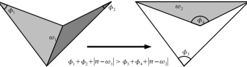
The first regularization technique, called Delaunay remeshing, is based on the fact that given a set of nodes, which are assumed to lie on the free boundary, there are many ways to connect them in order to form an approximating mesh. The objective is to find the mesh that has a minimal number of ‘thin triangles’, eg. triangles with very small angles. This can be achieved by beginning with an initial mesh and then performing a sequence of ‘edge flips’ (see Figure 1).
The second regularization technique addresses the phenomenon that nodes need to be constantly reallocated on the surface in order to maintain a (locally) uniform distribution. This can be achieved by treating the mesh as a system of masses (the nodes), whose position is restricted on the surface, connected by springs (the edges) with an extremely high damping constant [9]. Letting the nodes move under the influence of these spring forces for a certain time interval is called ‘relaxing the mesh’. Note that in order to have a measurable improvement of the quality of the mesh, we need to set the natural (relaxed) length of every spring equal to the local (minimal) radius of curvature.
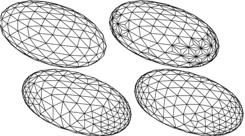
Although relaxation does improve the distribution of the nodes, it does not address the fact that when the local curvature increases at a region of the free boundary, the density of the nodes must increase accordingly for the mesh to resolve the developing geometrical feature satisfyingly. This can be achieved by refining the mesh, i.e. subdividing the faces of the mesh that are ‘too large’. A face is considered too large, and thus a candidate for subdivision, if its area is larger than a certain multiple of the area of an equilateral triangle with side equal to the local radius of curvature. The subdivision scheme that we use divides the triangular face into three new triangles by adding a new node close to the center of mass of the triangle and connecting it to the three existing vertices [28]. The new position of the new node is calculated using the osculating paraboloids from section 3.1 as a local representation of the surface. The refinement is always followed by remeshing and relaxation (see Figure 2).
Figure 2: Example of mesh regularization. Starting with a given mesh (top left), we refine the areas of high curvature (top right). After refining, we apply remeshing (bottom left) and relaxation (bottom right).
3.5
The code for axially symmetric configurations
The implementation of boundary element methods simplify notably when one considers an axially symmetric configuration. Firstly, the computation of the mean curvature, when writing the interface in the formz=h(r, t), has an explicit formula in terms of h(r, t) and its derivatives up to second order that can be computed using simple finite differences. Secondly, the integrals in the azimuthal angleθ that appear in (22) can be explicitly calculated as a previous step to discretizing the profile. These integrals may involve more or less complicated functions, such as elliptic integrals (cf. [23]), but are explicit in terms of them. The profile (r, h(r, t)) is then discretized in the form{(ri, h(ri, t)), i= 1, ..., N}and integrals are approximated in the same way as in the 3D
code, also using a singularity removal procedure. Nodes are moved influenced by artificial spring forces, as in the relaxation method explained above, so that they concentrate in regions of high curvature. The reduction in the dimension of the problem allows for a large number of mesh points and precise description of the “high curvature” regions up to several (typically 3 or 4) orders of magnitude of the curvature.
4
Evolution of axisymmetric drops
[13], [14], [27], and compare them with the equilibrium shapes obtained for long time behavior of evolving drops computed with the axisymmetric version of the boundary element algorithm. Later, we also present a stability analysis of equilibrium shapes and the possible formation of holes for drops evolving at constant Ω or constant
L.
4.1
Equilibrium shapes
The axisymmetric equilibrium shapes can be calculated in a closed form by integrating the differential equation
2κ=−Π +Bo 2 r
2
,
where Π = Π(2)−Π(1)is a constant. We describe the geometry of the drop by the functionh(r), which gives the
height of each point of the interface as a function of the distancerto the axis of rotation. Under the assumption of axial symmetry
2κ=−1
r d dr ( rhr √
1 +h2
r
) ,
and therefore we need to solve the equation
1 r d dr ( rhr √
1 +h2
r
)
=−Ω
2
2 r
2+ Π, (24)
subject to appropriate boundary conditions. If we assume a domain without holes and with a regular surface, then it is natural to imposehr(0) = 0 and equation (24) can be integrated once to yield
hr
√
1 +h2
r
=−Ω
2
8 r
3+Π
2r , (25)
which can be explicitly solved in terms of elliptic functions (see [19]). If the domain presents a hole of radiusa
near the axis, then integration of (24) leads to
rhr
√
1 +h2
r
−√ ahr(a)
1 + (hr(a))2
=−Ω
2
8 r
4+Π
2r
2+Ω
2
8 a
4−Π
2a
2,
so that, by imposing hr(a) = +∞one gets smooth toroidal solutions (that is, such that h(r)∼C(r−a)
1 2 as
r→a+) that we will call toroidal type I solutions, satisfying
hr
√
1 +h2
r
=
(
a+Ω82a4−Π2a2 )
r −
Ω2
8 r
3+Π
2r .
There is also the possibility that h(r) = 0 for 0 ≤r < a andh(a) = 0 with hr(a) = 0, so that the surface is
still smooth if one considers that a zero thickness film lies in the region 0≤r < a. These solutions have been thoroughly studied in [1]. We will call these solutions toroidal type II and they satisfy
hr
√
1 +h2
r
=
( Ω2
8 a
4−Π
2a
2)
r −
Ω2
8 r
3+Π
2r .
0 0.5 1 1.5 2 2.5 3 3.5 4 4.5 0 0.5 1 1.5 2 2.5 3 3.5 4 4.5
Angular Speed (Ω)
An gu lar M ome nt um ( L ) Spheroidal
Toroidal Type I Toroidal Type II
Ω∗
L∗
Analytical Solutions Evolution at constant Ω
Evolution at constantL
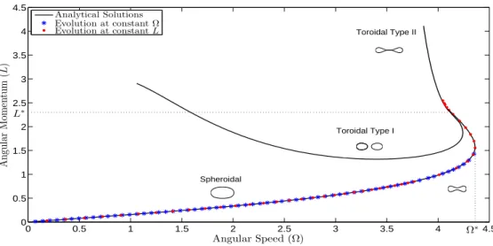
Figure 3: Bifurcation diagram of axisymmetric equilibrium shapes. TheoreticalL−Ω curves (continuous line) together with asymptotic values, for t→ ∞, of an initially spherical drop evolving at constant Ω (asterisks) or at constantL(dots).
4.2
Evolution at constant
Ω
When Ω is sufficiently small, starting from a spherical drop the evolution leads to an equilibrium shape in the family described in Figure 3 (some of those shapes are represented in figure 4-left). The condition that the drop’s volume is one leads, from (24), to the implicit equation
1 =V ol= 4π ∫ rmax
0
h(r)rdr=−2π ∫ rmax
0
hr(r)r2dr=
π
4
∫ rmax
0
Ω2r5−4Πr3 √
1−(Ω82r3−Π
2r
)2dr≡f(Ω,Π),
where rmax, is such that Ω
2
8 r
3
max− Π2rmax = 1. The equation f(Ω,Π) = 1 defines Ω as a function of Π. The
angular momentum can then be computed as
L= ΩI= 4πΩ
∫ rmax
0
h(r)r3dr=−πΩ
∫ rmax
0
hr(r)r4dr=
πΩ 8
∫ rmax
0
Ω2r7−4Πr5 √
1−(Ω2
8 r
3−Π
2r
)2dr ,
leading also toLas a function of Π. With (Ω(Π), L(Π)) one can represent the branch of spheroids in Figure 3. There exists a value of Ω, denoted by Ω∗ = 4.3648... such that axisymmetric equilibrium shapes do not exist for Ω>Ω∗ (this value has been computed numerically). Notice that for Ω<Ω∗ there is the possibility of two equilibrium solutions with the same Ω but differentL. We can easily compute the energy
E=A−1
2IΩ
2 ,
with
A= 4π ∫ rmax
0
r√1 +h2
r(r)dr= 4π
∫ rmax
0
r √
1−(Ω2
8 r
3−Π
2r
)2dr ,
and deduce (see figure 4-right) that those with smaller values ofLposses less energy and hence should be more stable. In fact, our numerical simulations verify this. When Ω>Ω∗, the drop’s surface becomes concave during the evolution. From this moment, mass is continuously evacuated from the neighborhood of the axis till a hole develops.
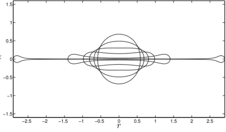
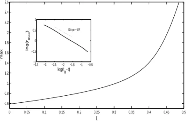
Once an equilibrium shape becomes unstable it undergoes evolution towards the formation of a singularity as discussed in [15]. The singularity is such that the drop evolves into a toroidal rim of fluid with a thin film inside (see Figure 5). According to [15], the radius of the toroidal rim grows as rmax = O((t0−t)−
1 2), i.e.
Figure 4: Left: equilibrium shapes for (Ω, L) = (0,0) , (3.14,0,61) , (4.09,1.05) , (4.36,1.57) , (4.29,1.91) , (4.09,2.38) (in order of higher eccentricity). Notice the existence of two different profiles for Ω = 4.09. Right: total energy as a function of Ω
of hmin(t) is characterized by a second kind self-similar solution hmin(t)∼O((t0−t)p(Ω)) withp= 4.1236 in
the limit Ω→ ∞ (or equivalently when surface tension is neglected and Bo→ ∞). In fact, the fact that rmax
diverges follows from the following argument in [15]. Assume that the shape consists of a disc of radius β(t) andr-dependent thicknessh(r, t), surrounded by a toroidal rim of radius of the tubeR(t); Then, the evolution can be described by the following thin film equations (see [15]):
∂h ∂t +
1
r ∂
∂r(rhv) = 0 (26)
4
h ∂ ∂r
( h r
∂ ∂r(rv)
) −2 v
hr ∂h
∂r = −Ω
2r+ 2
R(t)δ(r−β(t)) (27)
where v(r, t) is the radial velocity and δ is the Dirac delta function. The last term on the right-hand side of (27) models the force that the toroidal rim exerts on the film. If we search for self-similar solutions to (26), (27), from dimensional arguments one finds that they must have the form
h(r, t) = (t0−t)pf (
r(t0−t)
1 2
)
, v(r, t) = (t0−t)−
3 2g
(
r(t0−t)
1 2
)
(28)
wherepis a free parameter (depending on Ω). The solution (28) implies that the radius of the discβ(t) blows up at a rate (t0−t)−
1
2. Our numerical results for the growth of the drop’s sizermax, blowing up at the same
rate as β(t), support the result of [15] for the lubrication system (26), (27) (see Figure 6) up to the maximum drop extension reachable with our method.
0 0.05 0.1 0.15 0.2 0.25 0.3 0.35 0.4 0.45 0.5 0.6
0.8 1 1.2 1.4 1.6 1.8 2 2.2 2.4 2.6
t
rmax
−3.5 −3 −2.5 −2 −1.5 −1 −0.5 −1
−0.5 0 0.5 1
log(t0−t)
log(r
max
) Slope −1/2
Figure 6: Evolution of the equatorial radius of the drop at constant Ω = 10. Inset: log(rmax) vs. log(t0−t)
witht0≃0.51.
It is worth noting that these solutions representing a torus escaping to infinity in finite time cannot be a valid approximation to the real situation at all times. The reason is that velocity blows up at finite time and therefore inertial terms neglected under Stokes approximation will necessarily become dominant at some time. Then, the fluid particles will at most move with a centrifugal acceleration, so that their distancer(t) to the axis will verify
d2r(t)
dt2 ≃Ω 2r(t),
so that r(t) ≤CeΩt. Once a hole appears in the inner film, it will quickly retract and the resulting torus is subject of Plateau-Rayleigh instabilities leading to breakup into smaller droplets. The breakup of rotating torus will be discussed later.
4.3
Evolution at constant
L
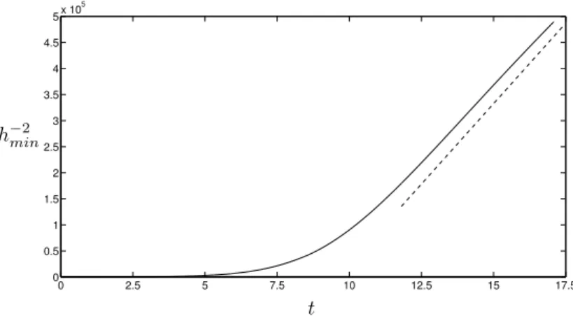
When the evolution of the drop takes place at constant angular momentum, as it is the case when the drop is mechanically isolated, and axial symmetry is imposed, we always converge to an equilibrium shape. Hence, all equilibrium solutions appear to be stable. There exists a subfamily of equilibrium solutions that we denoted as toroidal type II (see Figure 3) consisting of a zero thickness film connecting a toroidal rim. These solutions appear forL > L∗ withL∗= 2.3755. . . (see Figure 7). This value for the angular momentum was determined numerically taking into acount that its angular velocity pairing in theL−Ω bifurcation diagram is analytically known [27]. A natural question is then whether the zero thickness film (that is, the formation of a hole) develops in finite or infinite time for L > L∗ and if the hole develops in finite time, how the transition to the toroidal type I equilibrium solution with the same angular momentum takes place. Our numerical evidence is that convergence to the solutions with zero thickness film occurs at infinite time. This indicates that transition to toroidal type I solutions cannot take place. It is interesting to note that the thickness of the film follows an asymptotic law
hmin(t) =h(0, t)∼
C
√
t ,
and the profiles of the interface near the point where the film and toroidal rim meet present a very clear similarity law of the form
h(r, t)
hmin(t)
=f (
r−r0(t) √
hmin(t) )
, (29)
wheref(ξ) is a similarity profile such thatf(ξ)→1 asξ→ −∞andf(ξ)∼Aξ2 asξ→+∞. The radiusr0(t)
is such thatr0(t)→aast→ ∞whereais the radius of the film.
The evolution of the inner film can be easily described by means of an explicit solution of Stokes system that we compute next. For the sake of simplicity we restrict ourselves to the situation where no outer fluid is present. If one seeks for solutions to Stokes system in polar coordinates (cf. [17]) of the form
uz = αzr2+βz3, (30)
−1 −0.5 0 0.5 1 −0.8
−0.6 −0.4 −0.2 0 0.2 0.4 0.6 0.8
r z
Figure 7: Evolution of a drop at constantL= 2.54558 for timest= 0,1, . . . ,6 andµ1= 1, µ2= 0.1.
then it is simple to compute, from the condition∇ ·u= 0 , the relations
2γ+ 3β = 0,
4δ+α = 0,
so that
pr = (2γ−2α)r ,
pz = (4α−4γ)z ,
and therefore
p= (γ−α)(r2−2z2) . (32)
The boundary conditions for the balance between stress and capillary-centrifugal forces are, in the case of a planar interfacez=h(r, t) =hmin(t),
−p+ 2µ1∂uz
∂z = −
Ω2
2 r
2 ,
∂uz
∂r + ∂ur
∂z = 0,
so that plugging in (30)-(32) we obtain
−(γ−α)(r2−2h2)+ 2(αr2−2γh2) = −Ω
2
2 r
2,
2αzr+ 2γrz = 0,
resulting
α=−γ=−Ω
2
8 .
Since the center of the drop, atr= 0, moves in the vertical direction, it will follow
dhmin
dt =uz(r= 0, hmin) =βh
3
min=−
2 3
Ω2 8 h
3
min,
and we get
hmin(t)∼ √
6 Ω t
−1
2 , (33)
fort≫1.
Figure 8: Evolution of the inverse square of the film thickness at constant L= 2.54558 and comparison with straight line fort≫1.
(a) Profiles without rescaling. (b) Rescaled profiles.
Figure 9: Profiles near the region where the thin film and the rim meet fort≫1. In 9(a) profiles are depicted without scaling and in 9(b) the same profiles are represented after rescaling with the similarity law. Note that self-similarity behavior for constantL > L∗ shows convergence to toroidal type II solutions.
5
Evolution of drops in three dimensions
In the previous section we have discussed the evolution of axisymmetric rotating droplets both with constant Ω andL. We paid special attention to the development of instabilities and the possibility of topological changes. Of course, a natural question arises concerning the stability of all these results under perturbations that break the axial symmetry. This requires analysis and numerical computations of the evolution in generic 3D situations.
5.1
Evolution at constant
Ω
In the preceding section we showed that axisymmetric drops rotating at constant Ω, for Ω >Ω∗ evolve into the so-called (in the notation introduced by Howell et al. [15]) pizza shape. In the evolution, the film at the center tends to zero in finite time as shown in [15]. Whether or not these axisymmetric shapes are stable or, on the contrary, evolve towards a different configuration was mentioned as an open problem. With our boundary elements code, we found that indeed the expandedpizzaonly keep the axial symmetry when the angular velocity is sufficiently large, while for Ω < Ω2 ∈ (3.28,3.31)1 drops tend to axisymmetric equilibrium spheroids. For
Ω>Ω2 and Ω<Ωap∈ (4.55,4.59) an initially spherical drop evolves into an unstable peanut that elongates
infinitely in finite time. The drops become approximately axisymmetric about ther-axis and one can develop very easily a thin jet model of the type described in [10], consisting of the following equations (in the simplified situation where we have only one fluid, although this can be easily generalized):
1The value of Ω
3µ h2
∂ ∂r
( h2∂v
∂r ) = ∂Π ∂r ∂h ∂t + h 2 ∂v ∂r +v
∂h
∂r = 0
where
Π(r, t) =κ(r, t)−Ω
2
2 r
2≃ −Ω
2
2 r
2
and v(r, t) is the ur(r, z, t) component of the velocity field, which is, at leading order, independent of z and
dominant with respect to theuz component. Similarity solutions
h(r, t) = (t0−t)
α
f((t0−t)
β
r) , v(r, t) = (t0−t)
γ
g((t0−t)
β
r)
to this system such that volume is preserved requireα= 14,β = 12, γ=−32. Notice that surface tension forces become negligible with respect to centrifugal forces for these similarity solutions. The equations forf(ξ) and
g(ξ) are
Ω2ξ+3µ
f2
d dξ
( f2dg
dξ )
= 0
f2+ξd dξ(f
2)−2 d
dξ(f
2g) = 0
and one straightforwardly computes the solutions to be of the form
g(ξ) = ξ
2 , f(ξ) =Ce
−√Ω
3µξ .
The constantC must be chosen so that the drop has a volumeV, yielding
C=
√ VΩ
√
3µπ3 .
Capillary forces only enter into play at the tips of the peanut and result in the formation of a small droplet whose size decreases in time. As in the axisymmetric case, one cannot expect an infinite growth of the drop in finite time, since inertial terms in Navier-Stokes equations necessarily will be dominant before the drop spreads out to infinity. The result will be the growth up to some sufficiently large length and the appearance of Rayleigh-Plateau instabilities resulting in break-up of the elongated drop in smaller droplets.
If Ω>Ωapand Ω<Ωsp∈(4.69,4.73) the initial spheroid configuration evolves towards a non axisymmetric
pizza like shape (a torus with a thin film in the middle) that is also unstable. Finally for Ω>Ωsp the drop
degenerates into an axisymmetricpizza that evolves as described in the previous section. We have depicted the four cases in Figure 10.
5.2
Evolution at constant
L
It is well known, since the works of Brown and Scriven [6], that bifurcations breaking axial symmetry may take place at various values of L. For L =L2 ∈(0.65,0.66), axially symmetric shapes become unstable and
evolution may lead to equilibrium shapes with a 2-fold symmetry about the axis. We found that this is actually the case and forL > L2 but smaller than L∗2∈(1.06,1.10) evolution leads to the so-calledpeanut shapes. For
L > L∗2, interesting phenomena take place (see Figure 11). First, an initially spherical drop deforms into an axisymmetric shape. Nevertheless, these shapes are also unstable under non-axisymmetric perturbations and after some time destabilize and evolve very quickly towards thepeanut shape that is also unstable (sinceL > L∗2
and there are notpeanut-type equilibrium solutions) and breakup of the drop in several pieces takes place. It is worth to remark that centrifugal forces near the breakup point are subdominant with respect to viscous and capillary forces so that breakup occurs as theoretically described in [18] and [8]. With our code we were able to follow the evolution very close to the breakup point and we could even see the formation of two generations of necks (see Figure 12).
Figure 10: Shapes resulting from the evolution of the rotating drop at constant Ω: Ω<Ω2(top left), Ω2<Ω<
Ωap (top right), Ωap <Ω<Ωsp (bottom left) and Ω>Ωsp (bottom right). They are not at the same scale.
The values of Ω2, Ωapand Ωspare obtained numerically
0 5 10 15
0 5 10
Time
Ω
(a) Ω versus time forL= 1.41
(b)t= 2.36 (c)t= 8.11
(d)t= 12.36 (e)t= 14.16
Figure 12: On top, shape of the rotating drop at constantLnear the breakup point (t= 14.55) forL= 1.41,
µ1= 1 and µ2= 0.01. The original drop has transformed into two big drops with a cascade of necks between them. On bottom, detail of the necks. Observe the formation of small droplets in the smaller neck at the left.
leads to the formation of three necks emerging from the center of the drop, ending with smaller drops, and breaking up at a finite distance from the center (see Figure 13). We could not find solutions developing into a n-fold symmetry withn >3.
If we start with a torus as initial data, then for L < L∗2 there is a clear tendency to close the hole so that the drop tends to an equilibrium shape with the same topology as the sphere. On the contrary, forL > L∗2 the toroidal rim develops Rayleigh instabilities that lead to a break up into a sequence of drops (see Figure 14).
(a) Toroidal initial configuration (b) Equilibrium shape forL= 0.85
(c) Near the break-up point forL= 1.7 (d) Near the break-up point forL= 2.83
Figure 14: Different equilibrium or breakup configurations starting from a torus as initial data. In all cases
µ1=µ2= 0.5.
6
Conclusions
In this article we have studied the evolution of rotating viscous drops. We have developed a numerical algo-rithm based on the boundary integral formulation of Stokes system. The numerical algoalgo-rithm is adaptive and introduces automatically local refinement in the critical regions such as necks, where the drop is going to break up. Based on the numerical results and the analysis of the equations, we have described the evolution both at constant angular velocity Ω and constant angular momentumL. The different regimes found are summarized in tables I and II:
Table I: Axisymmetric evolution
Constant Ω ConstantL
Ω<Ω∗ Axisymmetric equilibrium L < L∗ Axisymmetric equilibrium Ω>Ω∗ Expanding pizzashape L > L∗ Toroidal Type II
The values for Ω∗ andL∗ have been determined numerically, Ω∗= 4.3648...,L∗= 2.3755. . .. Other critical values for Ω andL(Ω2, Ωap, Ωsp,L2,L3,L∗2 and L∗3) have been numerically computed for the particular case
Table II: 3D evolution
Constant Ω ConstantL
Ω<Ω2 Axisymmetric equilibrium L < L2Axisymmetric equilibrium
Ω2<Ω<Ωap Elongating filament L2< L < L∗2 stablepeanutshape
Ωap<Ω<ΩspAsymmetric expandingpizzashape L∗2< L < L∗3Breakup (2-fold)
Ω>ΩspAxisymmetric expandingpizzashape L > L∗3Breakup (3-fold)
The approach, at constant L > L∗, to the toroidal type II solutions occurs at an O(t−1/2) rate and the profiles for the interface present similarity features that we have described in detail. The elongating filaments at constant Ω reach an infinite length in finite time t0 and the length blows up at a O((t0−t)−
1/2
) and the interface profile approaches an explicit self-similar solution. Breakup at constant L is via an axisymmetric similarity profile of the type described by Lister and Stone [18] and Cohen et al. [8]. Finally, the axisymmetric expandingpizzashapes have a radius that grows at aO((t0−t)−
1/2
), as shown by Howell et al. [15].
A natural question that arises is whether the evolution for finite values of Ekman and Reynolds numbers presents different features to the limits considered in the present paper. This will be discussed in future publications.
Acknowledgements: This work has been financially supported by the project MTM2008-03255 from the Ministerio de Ciencia e Innovaci´on of Spain. The authors thankfully acknowledge the computer resources provided by the Centro de Supercomputaci´on de Galicia (CESGA) and the cluster Odisea from the Universidad Aut´onoma de Madrid.
References
[1] P. Ausillous, D. Qu´er´e, Shapes of rolling liquid drops, J. Fluid Mech., vol. 512 (2004), 133-151.
[2] A. Beer, Einleitung in die mathematische Theorie der Elasticit¨at und Capillarit¨at. A . Gisen Verlag, 1869.
[3] S. I. Betel´u, M. A. Fontelos, U. Kindel´an, O. Vantzos, Singularities on charged viscous droplets, Physics of Fluids 18 (5) (2006).
[4] N. Bohr, J. A. Wheeler, The mechanism of nuclear fission, Physical Review 56 (5) (1939), 426-450.
[5] M. Bonnet, Boundary integral equation methods for solids and fluids, Wiley 1995.
[6] R. A. Brown, L. E. Scriven, The shape and stability of rotating liquid drops. Proc. R. Soc. Lond. A 371 (1980), 331-357.
[7] S. Chandrasekhar, The stability of a rotating liquid drop, Proc. R. Soc. Lond. A 286 (1965), 1-26.
[8] I. Cohen, M. P. Brenner, J. Eggers, S. R. Nagel, Two Fluid Drop Snap-Off Problem: Experiments and Theory, Phys. Rev. Lett. 83-6 (1999), 1147-1140.
[9] V. Cristini, J. Blawzdziewicz, M. Loewenberg, An adaptive mesh algorithm for evolving surfaces: Simula-tions of drop breakup and coalescence, Journal of Computational Physics 168 (2001), 445-463.
[10] J. Eggers, E. Villermaux, Physics of liquid jets, Rep. Prog. Phys. 71 (2008), 036601.
[11] J. Eggers, M. A. Fontelos, The role of self-similarity in singularities of partial differential equations, Non-linearity, 22 (2009), R1-R44.
[12] M. A. Fontelos, U. Kindel´an, O. Vantzos, Evolution of neutral and charged droplets in an electric field, Physics of Fluids 20 (9) (2008).
[14] C. J. Heine, Computations of form and stability of rotating drops with finite elements, IMA Journal of Numerical Analysis 26 (2006), 723-751.
[15] P. D. Howell, B. Scheid, H. A. Stone, Newtonian pizza: spinning a viscous sheet, J. Fluid Mech., vol. 659 (2010), 1-23.
[16] M. Kallay, Computing the Moment of Inertia of a Solid Defined by a Triangle Mesh, Journal of Graphics, GPU, & Game Tools, vol. 11 (2) (2006).
[17] L. D. Landau and E. M. Lifshitz, Fluid Mechanics (Pergamon: Oxford, 1984).
[18] J. R. Lister and H. A. Stone, Capillary breakup of a viscous thread surrounded by another viscous fluid, Phys. Fluids 11 (1998), 2758.
[19] A. D. Myshkis, V. G. Babskii, N. D. Kopachevskii, L. A. Slobozhanin, A. D. Tyuptsov, Low-Gravity Fluid Mechanics, Springer-Verlag 1987.
[20] J. R. A. Pearson, Mechanics of Polymer Processing, Elsevier Applied Science Publishers (1985).
[21] J. Plateau, M´emoire sur les ph´enom`enes que pr´esente une masse liquide libre et soustraite `a l’action de la pesanteur, Rev. Univ. Brux., 16 (1843), 1-35.
[22] H. Poincar´e, Sur l’´equilibre d’une masse fluide anim´ee d’un mouvement de rotation, Acta Mathematica 7 (1885), 259–380.
[23] C. Pozrikidis, Boundary Integral Methods for Linearized Viscous Flow, Cambridge Texts in Applied Math-ematics, Cambridge University Press, 1992.
[24] H. M. Princen, I. Y. Z. Zia, S. G. Mason, Measurement of Interfacial Tension from the Shape of a Rotating Drop, Journal of Colloid and Interface Science 23 (1967), 99-107.
[25] J. M. Rallison, A. Acrivos, A numerical study of the deformation and burst of a viscous drop in an external flow, J. Fluid Mech 89 (1978), 191-200.
[26] F. Savart, M´emoire sur le choc d’une veine liquide lanc´ee contre un plan circulaire, Annales de Chimie 54 (1833), 56-87.
[27] D. R. Smith, J. E. Ross, Universal shapes and bifurcation for rotating incompressible fluid drops, Methods and Applications of Analysis 1 (2) (1994), 210-228.
[28] O. Vantzos, Mathematical modeling of charged liquid droplets: numerical simulation and stability analysis. MA Thesis, University of North Texas, Denton TX (2006).
[29] T. G. Wang, A. V. Anilkumar, C. P. Lee, K. C. Lin, Bifurcation of rotating liquid drops: results from USML-1 experiments in Space. J. Fluid Mech 276 (1994), 389-403.
[30] T. G. Wang, E. H. Trinh, A. P. Croonquist, D. D. Ellemant, Shapes of rotating free drops: spacelab experimental results. Phys. Rev. Lett. 56 (1986), 452-455.