Fault isolation schemes for a class of continuous-time stochastic dynamical systems

Fault isolation schemes for a class of continuous-time stochastic

dynamical systems

Ángela Castillo, Pedro J. Zufiria

A B S T R A C T

In this paper a new method for fault isolation in a class of continuous-time stochastic dynamical systems is proposed. The method is framed in the context of model-based analytical redundancy, consisting in the generation of a residual signal by means of a diagnostic observer, for its posterior analysis. Once a fault has been detected, and assuming some basic a priori knowledge about the set of possible failures in the plant, the isolation task is then formulated as a type of on-line statistical classification problem. The pro-posed isolation scheme employs in parallel different hypotheses tests on a statistic of the residual signal, one test for each possible fault. This isolation method is characterized by deriving for the unidimensional case, a sufficient isolability condition as well as an upperbound of the probability of missed isolation. Simulation examples illustrate the applicability of the proposed scheme.

1. Introduction

In the last three decades, system control theory has experienced an important evolution thanks to the advances on computer con-trol of complex processes (Astróm et al., 2001; Nise, 2011). Since the design of control systems is getting more systematic, the auto-matic task of responding to abnormal events in a process is becom-ing a new important challenge. This task gets more involved due to the confluence of an increasing complexity of modern plants and the need of quick diagnosis procedures (Blanke et al., 2003; Chiang et al., 2001; Korbicz et al., 2004). Hence, fault diagnosis schemes must be improved in order to reliably support human operators in the management of malfunctions. The problem of fault diagnosis involves the timely detection of an abnormal event (fault detec-tion), diagnosing its causal origins (fault isolation) and then taking appropriate supervisory control decisions and actions to bring the process back to a normal, safe, operating state (fault accommo-dation) (Ding, 2008; Iserman, 2006; Venkatasubramanian et al., 2003).

Fault Detection and Isolation (FDI) have deserved much atten-tion from different perspectives (Chen and Patton, 1999; Palade et al., 2006; Simani et al., 2003). In general, the analytical tools em-ployed so far for FDI can be classified into two main categories. On the one hand, stochastic discrete-time models inherited from the signal estimation and linear control fields have successfully

com-bined statistical schemes (mainly hypothesis testing) with geomet-rical tools in the design and characterization of FDI algorithms for linear systems (Basseville and Nikiforov, 1993; Gertler, 1998; Iser-man, 2006). On the other hand, deterministic continuous-time models coming from the adaptive and robust control community have proved to be suitable for nonlinear system modelling, where detection and isolation algorithms rely on the use of diagnostic observers to generate residuals whose profiles are evaluated (Al-eo rta-García and Frank, 1997; Frank, 1996; De Persis and Isidori, 2001; Polycarpou and Trunov, 2000; Zhang et al., 2005; Zhang et al., 2002). Recent research is also being focused on the design of diagnosis schemes for nonlinear discrete-time stochastic sys-tems either using computationally demanding particle filters (Tafazoli and Sun, 2006; Zhang et al., 2005) or adaptive estimators (Xu and Zhang, 2004).

The use of continuous-time stochastic models in system fault diagnosis provides a novel framework for taking into account sys-tem and sensor noises and disturbances, in order to construct new detection and isolation algorithms (Castillo et al., 2003; Castillo, 2006; Castillo and Zufiria, 2009; Münz and Zufiria, 2005; Münz and Zufiria, 2009). The seminal work in Castillo et al. (2003) devel-oped an initial study on both the detection and the isolation prob-lems. An extended characterization of the detection problem was later derived in Castillo and Zufiria (2009). The present paper accomplishes a parallel characterization task concerning the isola-tion problem.

the isolation problem. Although there are approaches which inte-grate detection and isolation in a unified process (see Venkatasubr-amanian et al., 2003 and references therein), typically, the fault detection and isolation tasks are accomplished sequentially: fault isolation goes into effect after a fault is detected, with the objective of determining the location/type of the fault (Zhang et al., 2005; Zhang et al., 2008). The fault isolation task is aimed to determine the particular type of fault among a set of known (or partially known) possible fault types, and to determine its location (the par-ticular faulty subcomponents among the set of all subcomponents under consideration) (Zhang et al., 2005; Zhang et al., 2008). This paper addresses only the discrimination of the actual and previ-ously detected fault among a list of possible faults in the system, been detected. This objective within such stochastic framework will naturally allow for the formulation of isolation as a classifica-tion or statistical decision task, or more generally, as a pattern rec-ognition problem (Bishop, 2006; Duda et al., 2001).

Precisely, the nominal part will be in general a nonlinear time-variant system, perturbed by a random process which character-izes the model uncertainty. Additive faults will be considered (both abrupt and incipient) and also modelled as random processes. In such context, the presented FI schemes exploit the model-based analytical redundancy by generating a residual via a diagnostic ob-server, along the line proposed in Zhang et al. (2002) for determin-istic nonlinear uncertain systems. Such residual defines the fundamental feature space where the fault classification task is to be performed.

It is worth mentioning that the whole residual-generation/ detection/isolation process can be interpreted as the typical se-quence of steps followed in a pattern recognition scheme (Bishop, 2006; Duda et al., 2001; Fukunaga, 1990): feature extraction, fea-ture selection and statistical classification. Hence the isolation pro-cess can be seen as a special type of pattern recognition problem.

Following standard statistical classification theory (Bishop, 2006; Duda et al., 2001; Fukunaga, 1990), two main FI schemes could be developed in such context. On the one hand, well known Bayes rule based methods could be applied, but they would require the assumption that a prior distribution of possible faults to be available. On the other hand, a hypothesis testing based set-up can be constructed; this second perspective is the one employed in this paper. Precisely, we develop a hypothesis testing set-up on continuous-time statistics of the residual; this method does not re-quire any a priori assumption and, despite that its main objective is to discriminate a fault from a previously given list, it can also alter-natively determine that the fault type is a new unknown one. The development of this approach and its posterior analysis has been founded upon the results in Castillo et al. (2003) where fault isola-tion was first presented, and (Castillo and Zufiria, 2009) where fault detection was rigorously characterized. Hence, the results pre-sented in this work, applied to fault isolation, extend and complete those in Castillo and Zufiria (2009) and Castillo et al. (2003).

The paper is organized as follows. In Section 2 the problem for-mulation is presented where the system model and possible faults are mathematically characterized. Then, the proposed FI scheme is put into a general context in Section 4.1, for its posterior analysis in Section 4.3. The practical validity of the proposed approach is illus-trated in Section 5 with two simulation examples addressing abrupt and incipient faults. Concluding remarks are finally exposed in Section 6.

2. Problem statement

In this section, the mathematical formulation is presented for both the class of systems under consideration as well as the types of possible faults which may affect the system.

Let us consider a general nonlinear time-variant dynamical sys-tem described by:

x(t) =/(x(t), u(t),t) + n(t) + B(t - Tom),

y(t) = h(x(t),u(t),t), (1) x(0) = x0,

where x(t) e Rn is the system state, which has known initial value

x0 e ttn;u(t) e Rm is the control input; the known function

/ : Rn x Rm x R+ -> R", / e C\ represents the dynamics of the

nom-inal model; B(t - T0) is a diagonal matrix representing the time

pro-file of the fault, and it is made up of the following functions as diagonal elements:

T0 being the unknown instant when the fault occurs and Q a

posi-tive value. Observe that for high values of Q¡ the function ft(t - T0)

will be similar to a step function. More specifically, in the case of an abrupt (sudden) fault, those functions will take the form of a step function and in the case of an incipient (slowly developing) fault they will be ramp-type functions; the fault process <f> -. R+ —> Rn

rep-resents the changes in the system dynamics due to a fault, it is as-sumed to be an n-dimensional stochastic process whose components are Gaussian generalized processes (Larson and Shu-bert, 1979); in particular the fault process components are defined as 4>¡(t) = X,(t) + bi(t)Wi(t), i = 1,..., n, where X,(t) is a continuous in mean squared (abbreviated MS-continuous) Gaussian random process, £>,{t) is a positive and square integrable deterministic func-tion and W,(t) is White Gaussian Noise (WGN). Detailed properties and implications of the Gaussian models can be found in Larson and Shubert (1979) and Duda et al. (2001). The uncertainty random vec-tor f] -. R+ —> R", which gathers external disturbances and modelling

errors, corresponds also to an n-dimensional stochastic process whose components are of the same type. Statistical independence between the uncertainty and the fault processes is also assumed. The derivatives of stochastic system (1) are interpreted as mean square (MS) derivatives.

Gaussian generalized processes (see Larson and Shubert, 1979) are considered in the model with the aim to account for the widest variety of cases, preserving the ubiquitous Gaussianity condition. The hypotheses of MS-continuity and WGN (see Larson and Shu-bert, 1979) are needed to assure the existence of the stochastic integrals involved in the isolation approach presented in this paper.

Finally y(t) e Rq is the measurable output, and the nonlinear

mapping h -. Rn x Rm x R —> Rq can represent different output

3. Residual generation

Once a fault is detected in the system, for instance applying the Fault Detection (FD) schemes proposed in Castillo and Zufiria (2009), the next step is to find out as much information as possible concerning such a fault, in order to fix it or at least to avoid its consequences.

The isolation scheme proposed here is based on the analysis of the residual signal obtained from the process plant and a diagnos-tic observer, since such residual gathers basic information about the fault affecting the system. The choice of the diagnostic observer will depend on the characteristics of the system, and it is aimed to get a residual as easy to analyze as possible. In Jiang et al. (2002), Li and Zhou (2004), Venkatasubramanian et al. (2003), Witczak et al. (2002), and Zhang et al. (2002) and references therein, the existing work on the design of appropriate diagnostic observers for fault detection and isolation is illustrated.

Taking into account the structure of system (1), a convenient diagnostic observer can be constructed following the basis of the Luenberger observer, that is, the diagnostic observer is determined by the nominal part of the model plus a stabilizing term (see Zhang et al., 2002; Castillo and Zufiria, 2009):

*(t) = ¿ ( x ( t ) - x ( t ) ) + / ( x ( t ) , u ( t ) , t ) , x ( 0 ) = x0, (2)

where x(t) e ttn is the state estimation and the matrix A is chosen

to be a diagonal matrix (for the sake of simplicity) with negative diagonal elements in order to assure the diagnostic observer con-vergence: A = diag(l! ln), with l¡ < 0, i = 1 n. In the

deter-ministic context, the selection of appropriate values for A has been addressed in Willsky (1976) and references therein; also, diag-nostic observers (2) have been improved to get faster FDI schemes (Li and Zhou, 2004). Here, as a first step, the basic structure is em-ployed looking for a simple compromise between fast response and numerical stability.

Note that since the state availability is assumed (see previous section), in (2) the function /(*(•), •, •) is used instead of/(x(-),-, •) as it would correspond to a proper Luenberger observer. Such sub-stitution does facilitate the residual generation.

Subtracting the diagnostic observer (2) from the system (1), and since the MS derivative is a linear operator, the differential equa-tions system explaining the evolution of the residual process e(t) = x(t) - x(t) is obtained, namely

é(t)=Ae(t)+t](t) + B(t-T0)^t), e(0) = 0. (3)

This residual process contains fundamental information con-cerning the fault, that is the existence or not of a fault in the plant and, in affirmative case, about the fault features. As it will be seen later, while there is no fault in the system (and t]{t) is a WGN) e(t) is a multidimensional Ornstein-Uhlenbeck stochastic process (Lar-son and Shubert, 1979), whose analysis has proved to be crucial in the detection procedure presented in Castillo and Zufiria (2009), and also constitutes the key of the isolation schemes presented here.

4. Isolation scheme

In this section we develop the proposed isolation scheme. We start considering some preliminary issues.

4.1. Preliminaries

The isolation scheme proposed in Section 4.3 is grounded on the following detection assumptions:

Assumption 4.1. The fault has been previously detected in the

plant modelled by system (1) with any detection method - see (Castillo and Zufiria, 2009) for an example - at the time instant Td.

Assumption 4.2. The detection time Td is close enough to the fault

occurrence time T0.

Concerning the isolation problem, the initial assumptions are:

Assumption 4.3. A list of possible faults is available:

{$1,$2,...,$,}, (4)

with known (except for T0) time profile functions ft¡(-), k = 1 /,

and totally determined fault processes 4>k{t), k = 1 /.

The probability distribution for each fault process <f>k{t) will be

denoted by p{<f>k{t); ^k) where <Pk is the label which determines

each fault. Hence, the corresponding moments or derived distribu-tions will follow the same notation (e.g., p(e(t); <Pk), £[e(t); <Pk],

etc.). In general, fe-th fault will be referred either by process <f>k{t)

or by its label <Pk.

Assumption 4.4. The faults in the list (4) can occur just one at a

time.

In practice, this assumption can be minimized if the isolation scheme is able to address unknown faults (e.g., the sum of known ones).

Assumption 4.5. The corresponding mean functions of the faults

in the list (4) are significantly different.

Finally, if a fault not belonging to such list is occurring, we will refer to that fault as "unknown fault".

The purpose of the isolation phase is to identify which one of the faults in the list is the one really acting in the system (or to con-clude that a possible non-registered fault has occurred).

The residual process (3), will have different characteristics depending on the occurrence time T0 and on which fault is acting

in the system. Assuming that the feth fault occurs, the residual will evolve according to the following equations

e,(t) = A,e,(t) + ti,(t) + pu(t - T0)¿w(t), e((0) = 0 , t > 0,

¿ e { l , . . . , n } ;

Note that the uncertainty on the value of T0 (which lies in the

essence of the quickest detection problem (Kailath and Poor, 1998; Poor and Hadjiliadis, 2009)) is not so relevant in this isola-tion formulaisola-tion, since a previous detecisola-tion step is being assumed. Hence, the value of T0 can be estimated (for instance t0 = T¿) so

that the residuals are to be considered since the detection of the fault, that is for t > Td. Solving those equations, in case fault <Pk

has occurred in the system at time I0, the residual components

re-sult in

e,(t)= / el^\{x)dx + [ e^-^hiix - T0)4>ki{x)dx,

Jo JT0

t^T0, i e { l , . . . , n };

or equivalently

e,(t)=ei(Ti)eUt-T¿ + f e^\(x)dx + / " < * < " % ( * - Ta)4>ki{x)dx,

•>Td ->Td t>Tit ¡ e { l , . . . , n };

Co

Jo Jo

JT0 JT0

£[e((t);*k] = ftex>^E[i1i(x)]dx+ f e>^ pki(x - T0)E[<¡>ki(x)]dx,

•JO JT„ i € {!,...,n},

and the covariance between two arbitrary components of the resid-ual vector (h and ¡2) under the hypothesis that fault <Pk is acting in

the system is

v(eh{U),e,l(t2)-<I>k)= i" / V ' ^ ^Cov(r]h(x,),r]h(x2))e1^ %i)dx2dxx

Jo Jo

PkH(i\-To)Cov(4>kh(x^,

4>kh(i2))Pkh(i2-To)eVt2 ^dx2dx,

+

j

f'

MH ^cov^x,),^.^))

Jo JT0

xh^i-To)^ ^dx

dx,

+ T f

e\<* ^p

(x,-T

)

JT0 JO

Cov(4>ki,(xx),t]h(x2))ek2lh ^>dx2dxx.

Assume now that the covariance matrices associated with the n-dimensional processes t]{t) and <f>k{t), respectively E^ti,t2) and

£Vk(ti, £2). are known. In addition, since we are assuming

indepen-dence between faults and the system uncertainty (see Section 2), the last two terms in the preceding covariance expression must be zero.

Therefore, the probability distribution followed by the residual stochastic process under the hypothesis that the fault <Pk is

affect-ing the system is given by: e(t)±jV(mk(t),Zk(t)),

where

/£[ei(t);**]\

mk(t)

and

W) =

\E[en(t);<l>k]J

I Var(e,(ty,0k) Cov{e^t),e2{t)-<l>k) ... Cov{e^{t),en{t)\^k)\

Coi>(ei(t),e2(t);<Pk) Var(e2(t);$k) ... Coi>(e2(t),e„(t);<Pk)

V

which characterize the distribution of e(t) on each instant of time, depending on the fault process 4>k{t) and the profile function

h(t - T0).

4.2. Statistical framework for detection and isolation

Under the assumptions in Section 2, the residual e(t) is, in the most simple case, a multidimensional Ornstein-Uhlenbeck (OU) stochastic process. Hence, although it can be statistically character-ized by the distribution provided above, the analysis of optimal detection and isolation schemes in such context is not straightfor-ward. In Zufiria (2012) time varying additive changes in such pro-cess are considered and the associated Likelihood Ratio (LR) is calculated, whose analytical expression is very cumbersome. In general, such complicated form of the LR makes optimal detection schemes to be computationally too expensive. In addition, such LR form does not allow a straightforward implementation of on-line schemes, as opposed, for instance, to the CUSUM schemes in the Brownian motion framework.

It is worth mentioning that the Generalized Likelihood Ratio (GLR) schemes proposed in Willsky and Jones (1976) for several types of additive faults in linear discrete-time Gaussian systems

serve as a good reference for the design of some detection/isolation schemes; nevertheless, they cannot be efficiently applied for contin-uous-time multivariable OU processes in a straightforward manner.

So far, practical FD schemes grounded on heuristic approaches have been successfully implemented (Castillo and Zufiria, 2009; Münz and Zufiria, 2009; Zufiria, 2009). Under some additional assumptions such as the availability of an estimate of T0, or a

par-tial knowledge of fault functions (e.g. their profile) it is possible to derive the approximations leading to the efficient isolation schemes proposed in this paper (see Zufiria (2012) for more details).

The scheme proposed here represents a natural extension of the fault detection method presented in Castillo and Zufiria (2009), by means of applying on the residual several hypothesis testing schemes in parallel, one for each possible fault; this method is spe-cially suitable for noticing faults which are not registered in the list (4).

Next, this isolation approach is analyzed. 4.3. Proposed isolation approach

The approach proposed here employs some ideas from previous works in discrete-time systems (Basseville and Nikiforov, 1993; Willsky, 1976; Willsky and Jones, 1976) since it is based on the application of several hypotheses tests. One can interpret the parametrized distributions p{e{t); <Pk) =p$ (e(t)) as likelihood

functions. If these functions were fully available, one could employ the corresponding likelihood ratios in order to optimally construct such tests. Unfortunately, these overall likelihood functions are very difficult to obtain in general. Their computation has been ad-dressed under some specific assumptions in Zufiria (2012), where the problems of classical detection and quickest detection (Kailath and Poor, 1998; Poor and Hadjiliadis, 2009) have been studied using also the residual e(t) of Eq. (3). In fact, the likelihood ratio be-tween the null (no fault) and the fault hypotheses is calculated there (generalizing some results in Arató (1982)) for the case of deterministic faults and fixed interval of time. Also in Zufiria (2012), this likelihood ratio is employed as the basis of some on-line suboptimal hypotheses tests for building fault detection schemes. Nevertheless, these results in Zufiria (2012) may not be easily extended to the general isolation problem, specially for the case of stochastic faults. In such case, the analysis strongly depends on the statistical characterization of the faults: for instance, when they are non-stationary or non-Gaussian processes, it seems that as far as we know only suboptimal isolation schemes can be effi-ciently designed. (Some specific cases, such as the detection and isolation of parametric faults have been addressed in Münz and Zufiria (2009), and a comparison of some existing schemes has also been performed in Zufiria (2009).)

In this work, the analysis performed in Section 4.1, provides the probability density functions p(e(t);<Pk) at each instant of time t.

Hence, based on the corresponding family of likelihood functions (one for each instant of time and each fault in the list (4)), different isolation schemes could be defined. For instance, isolation could be accomplished when p(e(t); <Pj) >p(e(t); <Pk), Vk^j during a

pre-scribed interval of time. Nevertheless, these schemes seem solely appropriate when only faults from the list (4), with a full statistical characterization, can happen.

fea-ture; so they have been also successfully employed in Castillo and Zufiria (2009). Under Assumption 4.5 the set of / simple tests

Hi : £[e(t)] = £[e(t); ^j • • • H<0 : £[e(t)] = E[e(t); *,]

H} : £[e(t)] * £[e(t); ^ ] • • -H* : £[e(t)] * £[e(r); *,],

can be applied to check if the actual residual mean corresponds to the expected mean when each one of the faults in the given list was affecting the system. Substituting <f>(t) by 4>k{t), k = 1 /, in

(3), the distribution of the residual given the occurrence of the kth fault can be determined, so that the mentioned hypotheses tests for the means {£[e(t); <P^] £[e(í);<P¡]} can be appropriately con-structed (Fukunaga, 1990; Gertler, 1998). Given the mean vectors and covariance matrices one can determine the tests acceptance re-gions following, for instance, the two strategies to construct a mul-tidimensional hypothesis test presented in Castillo and Zufiria (2009) (component by component and squared Mahalanobis distance (SM-distance) based strategies).

The test requires the construction of a mean estimator, /x(t) : R+ —> Rn, whose probability distribution must be

deter-mined, based on the distribution of the residual process assuming different faults. The acceptance region for each test, Bk(t),

k = 1 /, is obtained as a ball, which will depend on the selected test construction strategy, basically defined by a distance d(-, •), see (Castillo and Zufiria, 2009). Each ball Bk(t) will be centered in the

mean of the estimator under the hypothesis that the kth fault is occurring, E[¡i(t); <Pk],

Bk(t) = {U Rn/d(f,E[/i(t); **]) < ky}, (5)

being ky such that Bk(t) fulfills the condition

P(ji(t)eBk(t);0k) = \-y, (6)

where the predefined small value y is the test size.

For instance, in the unidimensional case, if choosing a Gaussian estimator ¡i(t)} for example one of the following

/ia(t) = e(t); m,{t)=\jo e{x)dx, t > 0 ;

¡ic(t) = i J^ e(x)dx, t > T; ¡id(t) = fo e»^e{x)dx, p < 0 (7)

(see Castillo and Zufiria (2009) for details), the acceptance regions corresponding to each fault are

(lk(t),uk(t)} = (E\M(t); *k] " hiy/Var(ji(t);$k),

x£[/i(t); $k] + hjvVarMt);**)], (8)

with k = 1 /. (hj_ is the normal distribution value such that P ( z < hi) = l - i )

Hence, provided a fault, <P = <Pj, from the list (4) happens, the realization of the residual mean estimator will remain between the limits of the test corresponding to such actual fault <Pj with probability 1 - y, and hopefully outside the acceptance regions associated with the rest of the tests.

On the other hand, provided a fault <P, which is not in the list (4) happens, the realization of the estimator will presumably end up outside the acceptance regions associated with all the faults in list (4). In this case the proposed isolation method will be useful to advertise that an unknown fault has appeared in the system.

Therefore, based on the specified bank of tests, the proposed isolation decision scheme is grounded on the following definition:

Definition 4.1. T\so is the first (in the infimum sense) instant of

time for which either

(1) fi(t) e Bj(t) and fi(t) 4 Bk(t), Vk e {1,...,/} - {/}, Vt e [T>SO

-At, T'iso]. If there exists such Viso, then it is considered that the

j'-th fault in (4) is affecting the system (1), and T\so is the

iso-lation time instant for that particular estimator realization. (2) ¡i(t) i Bk(t), Vk e { 1 , . . . , /}, Vt e [T{0 - St, TQ . If there

exists such T\so, then it is considered that an unknown fault

is affecting the system (1), and T\so is the isolation time

instant for that particular estimator realization.

(Note: the increments of time At and St are parameters whose values must be fixed previously).

In the following we will consider the case a fault in the list (4) is happening, that is T\so will correspond to the first item of Definition

4.1. Then, T]so is determined as follows:

Proposition 4.1. Assuming a fault of list (4) is affecting the system,

let it be

Bo(t) = (uLA(t))

,

and

V = {?> rd/Vt e [ T - At,T],/i(t) e Bj{t) n fuUB*(t)) }•

Hence

T{S0 = MV.

T'iso will depend on the size of the intersection region among the

different acceptance regions, which could be quite big in case there is not much difference among the faults processes means: the most the faults differ the quickest is the isolation. Note that if there were not much difference among the faults means, the realization of the residual process might remain between the limits of the tests cor-responding to more than a single fault <Pk from the list (4), with a

significant probability. In such case, one would need to resort to the comparison between the corresponding likelihoods p^ (e(t)) in order to isolate the fault. Time T'iso will also depend on the time

in which the residual realization gets its steady state; hence, high values of | ¿¡I (lt being the observer stabilizing parameter) are

desir-able to speed up the convergence to the steady state of the residual sample path. On the other hand, \X¡\ must be small enough to guar-antee convergence of the computational numerical methods em-ployed for solving the differential equations; this leads to a trade-off.

We proceed now to characterize and analyze the presented iso-lation scheme for unidimensional systems as well as for multidi-mensional systems where only one component of the residual is considered: some analytical sufficient conditions which guarantee, with significant probability, the isolability of a fault from a prede-fined set, are given in Section 4.4. Besides that, the probability of missed isolation, for unidimensional systems under certain condi-tions, is studied in Section 4.5.

4.4. Isolability conditions for unidimensional systems

The results presented here for unidimensional systems are also valid for multidimensional systems where only one component of the residual is considered.

Let us define now an upperbound (in probabilistic sense) for the random variable T'iso, the instant of time when fault <Pj is isolated

among the faults of set {<P^ <P¡}.

Definition 4.2. fJ¿ = At + inf{T > Td/Wt > T Bj(t)nBk(t) = ill}.

Definition 4.3. t{0 = At + inf{T > rd/Vt > T B,(t) n (Une{i ¡}_

Proposition 4.2. Observe that

ÍL = niax{7£, k = \,...,lMi}

Definition 4.4. If f\so < +00 then fault 4>¡ is said to be f{.0-isolable.

Definition 4.5. If t\so = +00 then fault 4>¡ is said to be hardly iso-lable from the set of faults {4>^ 4>i}

Lemma 4.1. If a fault <Pj is t\so-isolable then t\so is an upperbound in

probabilistic sense, namely with certain probability, for T\so, the

isola-tion time instant of fault <Pj. That is

P(tl e TJ; 0¡) = 1 - P(n(t) íBj(t) for some t e \PiS0 - At, t'iso\ • Q¡).

Observe that

• T'iso depends on each particular mean estimator realization, that

is T\so is a random variable, whereas t\so is a deterministic value.

• TJ is the set defined in Proposition 4.1.

• P(fi(t) 4 Bj(t) for some t e lt]so - At, f-j 1; <P¡\ can be

upper-bounded (for systems fulfilling Assumption 4.6) following the reasoning in Subsection 4.5.

Proof. By construction of the jth acceptance region B,{t) and the

definition of T'iso,

V

p(vt€p

-At,7t

],Mt)eBS(t)nB5(t)...nB,(t)n...Bf(t);*,) =

p(vt€p

-At,7y,Mt)ei%(t);*j) =

1 - P[fi(t) íB,{t) for some t e \f{0 - At, 7 ^ ] ; *, D

Next, based on the isolability concept, we develop a sufficient condition, aimed to guarantee, with certain probability, a fault isolation by the proposed scheme.

Theorem 4.1 (Isolability sufficient condition). Let us consider

(a) The time profile functions of two faults (¡>¡ and <Pk, that is

• 0 if t < To

and

0 if t < To (0

iit-W - ^ H i - ^ e - . ) ift

e*(t-To) =

1 _ e-stíf-To) if t > To

(where Q¡, Qk > 0);

(b) The corresponding random processes <pj(t) and <pk(t) such that

/j,(t - T0)£[^(t)] - ft(t - T0)£[^(t)] > 0 Vt e [T0, T0] and

/j,(t - T0)£[^(t)] - ft(t - T0)£[^(t)] > £ Vt > r ; (9)

e > roc(/l) limsup (h^Jvar(jj.c(t); &¡) + h^Jvar^t); &k)\ (11)

where

roa(/l) = - 1 , tt»¡,(/l) = -X, (oc(X) = - 1 , cod(X) = Ap.

Observe that mc(X) >0, Vf e {a, fa, c, d}.

(Note: X is the observer gain in the unidimensional case, and p the parameter in the expression of estimator ¡id.)

Proof. For the sake of simplicity let us choose for example

estima-tor ¡ia(t) = ¡i(t) = e(t) and condition (9) to delineate the main steps

of the proof. • First, since

/i(t) = e ( t ) = / eMt-^T¡(x)dx + [ eMt-^p(x - T0)cj>(x)dx, t

Jo JT0

and taking into account the linearity of the mean operator, E[/í(t);*,]-E[/í(t);*k]= / e

IT, «•'-^Elfijix - T

0)4,(T)

ft((T - T0)<j>k(x)]dx, t > T0,

meaning that the estimator expectations assuming fault í>¡ and fault <Pk differ in an integral term depending on the difference

be-tween the means of the corresponding fault processes ft(t - T0)4>j{t)

and f¡k(t - T0)4>k(t). (This is also the case for estimators ¡ib, ¡ic and

Hd-)

• Assumption (9) implies

E[^t);0i\-E[^t);0k\= e ^ E ^ T - T o ) ^ ) - &(t-T0)^(T)]dT-t

°^-^¿Ji=wr

(The diagonal arrow / indicates that the function ^ ( 1 -ei(t~T|J>)

grows up monotonically towards the value A¡.)

• This result, along with condition (11), implies that 3t* > T*0

ful-filling that Vt > £*

(1 - e ^ -1» ) ) > (h^Var(pL(t); <P¡) + hy_^/Var(^i(t); <Pk)

and so at* > T'Q such that Vt > t*

E\M{t);0j] -E[ji(t)-$k] > (his/var(n(t)\ty) + h^VarQUt); <¡>k)).

(12)

Therefore, remembering (lk(t),uk(t)] as defined in (8):

inf{r Ss T0/yt Ss T B)(t) nBk(t) =0} = inf{r 5, T0/yt 5, % /¡(t) Ss uk(t)} =

inf{TssTo/Vt ssT E^O^I-hiyVarMt);^) Ss£[/i(t);á>,;] +h?V^añ^tt)^)} =

inf{Tssr0/Vt ssT E[íí(t);<f«¡]-£[/i(t);á>,J ssfiiV/l'ar(;u(t);á>i)+fi|v/^'-(/i(t);á>,í)}<r

/?j(t - T0)£[^(t)] - ft(t - T0)£[^(t)] < 0 Vt e [T0, TJ] and

/J,(t - T0)£[^(t)] - ft((t - T0)£[^(t)] < - £ Vt > r0; (10)

Then, a sufficient condition to assure the existence of a finite value

T'iso > ro such that the fault ®i Siven by P0 - To)<Pj(t) is tf0-isolable

by the Fl scheme associated with estimator ¡i^(t), f e {a, b, c, d} (see Definition 4.1 and estimator proposals in Eq. (7)), is that

3ÍJ¿o = At + inf{T > To/Vt > T Bj(t) n Bk(i) = 0} < At + t* < +00.

We conclude that the fault 4>¡ is r¡¿-isolable from the set {4>¡, <Pk} by the isolation scheme described in this section (see

Defini-tion 4.1) corresponding to estimator ¡i(t).

Note that we can analytically determine the value of f\f0 solving

ls(T) = uk(T).

That is possible thanks to the continuity of functions uk{t) and

m

E\pi(T); n ~ EM?); **] = h^Var(p(T); *,) + h^Var(MT); <Pk),

when solving this equality it could be f sg T0, in that case

p¿a = T0 + At; or f > T0, and then t>¿ = t + At. Obviously t>¿ - T0

will be an upperbound of the time to be taken in the isolation of fault <Pj versus <Pk.

For the cases fulfilling assumption (10), we follow the same reasoning using

inf{r > To/Vt > T Uj(t) < lk(t)}

instead.

The same guidelines allow to prove the theorem for the rest of estimators ^ ( t ) , f e {b,c,d}. D

Corollary 4.1. I/the isolability sufficient condition given in Theorem

4.1 fulfills for k e { ? , . . . , / } - {/'} then 3rjso and ¡t ¡s

7Í = m a x | r ! i , k = l , . . . , i ,

M/} < oo,

An example of isolation in a unidimensional system, using the method just explained, is given in Section 5.2.

4.5. Missed isolation probability

According to Definition 4.1, the probability of missed isolation of the actual fault <Pj in a time interval is

P(p.(t) $ Bj(t) for some t e [T - At, 7]; &j)

= P(d(/i(t),E[/i(t); &j]) > ky{t) for some t&[T- At, 7]; <*>,•).

For unidimensional systems, with a Gaussian mean estimator MO.

d(/i(t),E[/i(t); *,]) = dM(n(t),E[n(t); *,])

_ | / i ( t ) - £ [ M t ) ; ^ ] l

^Var(n(t);^) ' (13)

and kj = fc.

A bound for the probability of missed isolation in an interval is calculated below, but under the assumption that the uncertainty process t]{t) and the fault process <j>(t) fulfill the following (memoryless in mean) condition.

Assumption 4.6.

E[f](t)lf]('Q),0 < £ < t] = E{t](t)\ Vt e 0

E 0 ( t ) / ¿ ( { ) , O < { < r ] = E 0 ( t ) ] V t e l

(14) (15)

Assumption 4.7. The uncertainty process i]() and the fault process

<p(-) are statistically independent (as established previously in Section 2).

Theorem 4.2 (Missed isolation probability upperbound). As a

conse-quence of Assumptions 4.6 and 4.7 the following results are derived for unidimensional systems.

(1) For estimator ¡ia(t) = e(t)

P(fJ.a(t) $ Bj(t) for some t e [T - At, 7]; <Pj)

= p(|/ifl(t)-£(/ifl(t);0>j)| > hiy/Var(jia{t);^),

for some t e [T - At, 7]; <£,-) < - TVari^T);^)

'[T-At.7]

(2) For estimator /xb(t) = \ fQ e{x)dx

P(pb(t) $ Bj(t) for some t € [T - At, 7]; <Pj)

= p{\Hb(t)-EUib{t);0j)\ > h^Var{nb(t);<Pi),

for some t e [T - At, 7]; <£,-) T2Viar(^(T);4>j)

2

m[T-At,7]

where m ^ ^ j = min lthi^/Var(pb(t); <Pj), t e [TUT2]\.

(3) And for estimator fj.d(t) = /0te'><t-T'e(T)dT

P(p(t) $ Bj(t) for some t&[T- At, 7]; <£>,•)

= p(|/id(t)-£[/id(t);0>j]| > hyJVar(N(t); *,),

for some í e [T - At, 7]; <£,-) e - ^ V a r O ^ T ) ; * , )

'[T-At.7]

where, in this case, m[TuTl] = rnin ^ " ' ' ' ^ ^ ^ ^ ¿ ( t ) ; <P,-), t e [7"i, I2] | .

Proof. See Appendix A. D

5. Examples

The proposed FI methods are illustrated with the following two examples.

5.1. Unidimensional example

This example illustrates the application of the proposed FI scheme as well as the isolability conditions on unidimensional sys-tems with incipient faults.

Consider the system given by the differential equation: x(t) = sinx(t)+i/(t) + ^ ( t - T o ) ^ ( t )

y ( t ) = x ( t ) , x(0) = 0,

where r¡{t) and v(t) are independent WGN processes with zero mean and autocorrelation functions Rn{U, t2) = ff?á(íi - 12) and

Rv(t-¡,t2) = o2v&{U -12), respectively. The fault in this simulation

will occur at time T0 = 70 and it is an incipient fault with the time

profile function

P(t~To) = 0 _{1 _} if t < T0

e-P(t-To) ¡f t > J

In this simulation example p = 0.05.

The diagnostic observer presented in Section 3 will be x(t) = l(x(t) - x(t)) + sinx(t),

x(0) = 0,

with X < 0 (for instance X = -0.5 is taken). Then subtracting model and diagnostic observer equations the residual equation

ISOLATION I

time

0

o

o

0

Q

0

n

ISOLATION II

i i i i i i i \y / / x + * /

y * x

/ * /

/ ^ /

/ •* /

/ > /

/ * /

/ * /

/ * /

— /^ • * /

/*" / / > y

X * / / + /

/ ** /

/ ' /

- / ' /

_{/ ' /}

/ / /

/ ' /

/ • / X *" X

/ ' /

/ / /

/ * X X * /

^X / . / / • * * * / ^ ^ A'z{\)/

X* /

/ /• /

/ ^ /

/ • /

X * /

U2» / / /

/ «*• /

/> "* /^

/ <* /

/ * /

/ ^ /

1 1 1 1 1 1 1 1

180 182 184 186 188 190 192 194 196 198 time

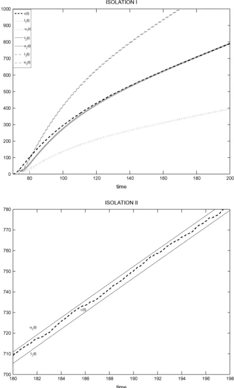
Fig. 1. Isolation: Bank of hypotheses tests. Unidimensional example.

is obtained.

We have simulated the occurrence of fault <P2 given by fault

function <fo(t) = 2t+ v(t). Applying one of the Fault Detection schemes proposed in Castillo and Zufiria (2009) the fault is de-tected at time Td = 73.67.

Once the presence of a fault is detected in plant, the next step is to isolate it. Let us establish the following set of possible fault processes

{^(t) = t + v(t), <fe(t)=2t + v(t), <fe(t)=3t + v(t)},

or equivalently: 4>k{t) = kt+ v(t), k = \, 2, 3, where v(t) is, as

said before, a WGN process independent of the WGN process

nit)-In order to isolate the fault, the residual process distribution is needed for the cases when each one of the possible faults was hap-pening. In this case the residual is

e(t) = e{TM<*<-"> + )r]{x)dx

Td

">f¡{T-T0)4>k{T)dT, t>Td,

where the value £{Td,tk} is the measured value of the residual

process at time Td under assumption the fault 4>k is affecting

E[e{t);<l>k] = e<TMe«-t-T¿

t

= £{T[|,#lt}eA

- ke-p<t-To)

1

T, 1

(-xy

i

- keMt-T«}

(-xy

<* + P) (X + pf

Ti

. \{eHt-Tá)-p(Tá-Ta)

(X + pf -{¿- + P)

Observe that for high values of t, namely asymptotically, t 1

E[e(t);0,

(-xy

Note that since

0 < / ? ( t - T

) £ [ ^ ( t ) - ^ ( t ) ] / +oo, fc<j, fc,j = 1,2,3,

t-^+co

the isolability sufficient condition (see Theorem 4.1) is clearly satis-fied, so that we have a guarantee that the isolation approach pre-sented in Section 4.3 is able to isolate any fault 4>k from the rest of faults in the list.

Since t](t) and v(t) are independent and zero mean processes then:

Cozv»(ti,t2) = Covn(tut2) + p(U - TojCov^tuW^ - T0)

= fi^t!, t2) + f$(U - T0)Rv(U,t2)f$(t2 - To).

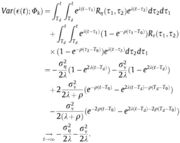
Therefore the variance of e(t), depending on <Pk is given by

Var(e(t);<Pk)= f f e'<t-^R,l(x1,x2)eMt-^dx2dx1

+ f [ eMt-x^ (1 - e-P^-T^)Rv(xux2)

hi hi

x (1 -e-P^-T°>)e^t-^>dx2dxi

an n _p¿Ht-Ti)\_a±r[ _p2i(t-Ti>

•ÚV-*

V - d - ^

+ 2X + p( >

2(X + pf >

t^co 2X 2.X

The preceding expressions are valid when the diagnostic obser-ver design parameter X 4 {—P,~Y}, where p is the fault time profile parameter. This is the case for this particular example because \X\ > p. Since the fault occurrence time T0 is unknown, it is

substi-tuted in the given expressions by the detection time Id; therefore,

for the sake of accuracy, it is important to consider a quick detec-tion method.

The approximations in this example must take into account the time the estimator takes in reaching its steady state, for instance in computing P¿; an estimation of such time should be added to rep-resent a real upperbound of the isolation time.

The acceptance regions corresponding to a collection of tests on the residual mean (one for each fault) are the basis of the isolation scheme. The acceptance region of the hypothesis testing scheme corresponding to the feth fault, considering the raw estimator p(t) = e(t) and the test size y = 0.05, results in

(lk,uk] = (E[e(t);<Pk] -i.96^Var(e(ty,<Pk),E[e(t);<Pk]

+1.96v/Var(e(t);«Plk)].

In this example, tests acceptance regions are simulated in stea-dy state, so that their intersection from Td is empty; hence, the

iso-lation time will be upperbounded by Td + At + Tss, being Tss an

approximation of the time the estimator takes in reaching its stea-dy state.

Fig. 1 shows, in two different scales, the time evolution of the estimator realization and the acceptance regions. As expected, the residual realization e(t), once it gets its steady state, remains between the test limits corresponding to <P2, and outside from

the limits determined by the rest of tests, as it can be seen in Fig. 1 (up). Notice that initially the error crosses the acceptance region of the test corresponding to fault <P^. It is necessary to wait until about riso = 180, the instant of time in which it is clear that

the error remains uniquely in the acceptance region associated with <P2 (see Fig. 1 (down)).

5.2. Bidimensional example

This example illustrates the application of the proposed multi-dimensional FI approach, based on the SM-distance, to a bidimen-sional system.

The example consists of a circuit with a nonlinear resistor, an inductor and a capacitor joined in parallel to a noisy resistor (see Fig. 2). We consider that the circuit is in space or belongs to a nu-clear plant, so that it could suffer two types of fault as a conse-quence of a radiation.

The system equations are:

dVc(t)

R

i(t) • _T¿3W

1

_v

_{+Í>7(t) + A}

_(r-r

_)<Mt)

dt =J

(t)+¿nt) + ft

(t-r

)fe(t)

y(t)-

m

y(0)- Qct.

At time I0 = 50 (known for the simulation but obviously

un-known for FDI tasks) a fault <Pk occurs in the system; we consider

that such fault can be one of the two {<P^, <P2}, given by the profile

functions

/ ?

( t - r

) =

if t < To if t > To '

fe(t-T

) =

. 1 if t > T0 '

and the fault functions

fait)'-

M((t-To)-i)v(t)

h A A

The random processes i](t) and v(t) are mutually independent, and they are distributed as WGN, with zero mean and autocorrela-tion funcautocorrela-tion

^WGN(íl;Í2) = "wGN^C-l — £2);

where, for the sake of simplicity, a* = a\ = 1. Also, R = L = C = M= 1 (in their corresponding units), V0 = 7 and Q = 0.01 were chosen for

the simulation,

Fault <P^ represents an incipient fault in the circuit provoked by the effect of radiation whose consequences show as a decrease in the initial constant voltage generated by the source voltage under healthy conditions. Abrupt fault <P2 could be caused due to a

change in temperature around the capacitor, changing so the intensity of the thermal noise generated in the capacitor noisy resistor (from a constant value to a function evolving with time).

Following the indications of Section 3 we take the diagnostic observer,

d

| l = -iVc(

)-f¿(

)-f¿

(

)

^

l

í

.

^ c ( t ) = li ( t ).

dt

m- m

Vc(t)

-HVc(t)-Vc(t))

Oct.

with l-i = X2 = -0.5.

Subtracting model and observer, the equations defining the residual vector given by the components

e1(t) = i(t)-i(t),

become dei(t)

e2(t) = Vc(t)-Vc(t)

dt de2(t)

dt e(t) =

^ i e i ( t )

-• he2(t)

-ei(t)

e2(t)

e(0) =

ft

(t-r

)^

(t)

ft

(t-r

)fe(t)

0 ,

0

I . o<t.

This system is linear and uncoupled, so that each one of its dif-ferential equations can be solved separately.

Under the given assumptions on the stochastic processes r¡(t) and v(t), the residual e(t) will be a bivariate Gaussian random pro-cess (totally determined by its mean vector and covariance matrix) and it can be written as

e(t)

JÍ^('-)(lv(T)--Ad(T-r0)<MT))dT

-Aa(T-r0)<MT))dT

For the sake of a compromise between performance and effi-ciency we have chosen the mean estimator

H(t) = ift_Te1(x)dx \ ft_Te2{x)dx

where the window size T has been set to 10 for simulations. This process inherits the Gaussianity of the residual process due to the linearity of the integral. Therefore, in order to draw the pro-posed FI scheme, that is to determine the SM-distance corre-sponding to each possible fault, we determine the mean vector and the inverse of the covariance matrix for the estimator process:

E\ji{t); 4>k} l£_

TE[ei(T);<Pk]dT

¡¡l

E[e

(xy,$

]dx

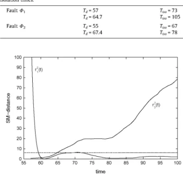
Table 1 Isolation times.

Fault tp]

Fault <PT

57 64.7 55 67.4

T

'ISO

T

'ISO

T

'ISO

T

= 73 = 105

= 67 = 78

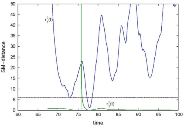
Fig. 3. Isolation: Bidimensional example. Fault <Pi. Td = 57.

120 140 time

Fig. 4. Isolation: Bidimensional example. Fault <Pi. Td = 64.7.

55-Fig. 6. Isolation: Bidimensional example. Fault <P2- Td = 67.4.

= = 2 / / Cov(eh(x1),ei2(x2))dx2dx1 ! ' I , Í2É { 1 , 2 } , I Jti-T Jt2-T

Coviu 0 )<t t) = (C^iitlViitY'®*) c°v(f¿i(t),fh(t);$k)

to finally determine the SM-distance

r2k(t) = (n(t) -E[^(t);<I>k])'Cov-\p;<I>k)(t,t)(Mt) -£[Mt);<*>/<]).

(The corresponding specific expressions are computed in Appendix B.)

5.2.3. Simulation results

In order to determine the regions defined in (5) (see Section 4.3) where ky is such that Bk(t) fulfills the condition (6), the test size has

been predefined to y = 0.05, being so ky = -2/n(0.05) ss 6.

This example has been simulated for two detection methods with different response time, and the isolation method proposed in this work, using the SM-distance. The results are summarized in the following Table 1 and Figs. 3-6.

Note that the isolation method works even in case of large detection times; besides, as expected, this approach takes more time in isolating the incipient fault <P1} specially for the case of

slow detection.

Also, as a consequence of approximating T0 = 50 by Td (different

in each case) the computation of the SM-distance suffers a tran-sient phase, as it can be seen in Figs. 3-6.

6. Conclusion

In this paper the Fault Isolation task for a class of nonlinear sto-chastic dynamical systems has been addressed. A new fault isola-tion stochastic method has been proposed and framed in the context of statistical classification theory. Based on a model-based analytical redundancy scheme, a residual signal is obtained via a diagnostic observer, for its posterior analysis. Then the method determines the fault affecting the system through the application of a bank of hypotheses tests in parallel, one for each possible fault. This approach allows for the derivation of a rigorous isolability suf-ficient condition.

The method has been illustrated in two simulation examples corresponding respectively to unidimensional and bidimensional systems, where the isolation of both incipient and abrupt faults has been accomplished.

Acknowledgements

This work has been partially supported by projects MTM2010-15102 of Ministerio de Ciencia e Innovación, CCG10-UPM/ESP-5236 of Comunidad de Madrid/UPM, and Ayuda Q.10 0930-144 of the Universidad Politécnica de Madrid (UPM), Spain.

Appendix A. Proof of Theorem 4.2

We address the simplest mean estimator /i(t) = e(t).

When a fault <P is affecting the system, such estimator can be written as the product of a deterministic function and a stochastic process

e(r) = / «•*«-*>(J/(T) + /?(T - T0)4,{x))dx

Jo

= eit i e->^r¡(x) + fi(x -T0)<j>(x))dx,

Jo by naming

Y(t)= f e-*(n(x)+p(t-T0)4>(x))dx

Jo

the estimator can be rewritten as ¡i{t)=euY{t).

Due to (14) and (15) we first prove that process Z(t) = Y(t) - E[Y(t)] is a martingale (Larson and Shubert, 1979). As a consequence the probability of missed isolation in the interval [ I - At,I] will be bounded.

Z(t) can be expressed as

Z(t) = f e-*(i/(T) + pit - T0)<KT) - E[JJ(T) + Pit - ToHix)])dx. Jo

Let Tt be the er-algebra generated by {(Í7(T),0(T)),O < x < t} (Billingsley, 1995). So,

£[Z(t + At)/^t]

= E[£e lt(.m + W-ToMx) -EWx) + fl(t-T0)4>(x)])dx

/

t+At "I

e a(n(x) + fi(t - T0)4>(x) - E[n(x) + fi(t - T0)4>(x)])dx/^

= E^e^(t,(x) + íl(t-T0)4>(x)-E[t,(x) + íl(t-T0)4>(x)])dx/^

/

t+At

e *EMx) + ¡}(t - ToM-c) -E[n(x) + ¡}(t - T0)4>(x)]/Ft]dx = Z(t)

/

t+At

e aE[n(x) + fi(t - T0)4>(x) - E[n(x) + /?(t - T0)4>(x)]]dx

= Z(t) + 0=Z(t),

that is, Zit) is a martingale respect to the cr-algebra Tt.

Note that since Z() depends on r\{-) and on <£(•), then the asso-ciated cr-algebra satisfies

<7({Z(T), 0 < X < t}) C Tt,

and by the martingales properties, if Zit) is a martingale with re-spect to Tt then it is also a martingale with respect to a smaller

cr-algebra (Billingsley, 1995), that is Zit) is a martingale with re-spect to CT({Z(T), 0 sg T sg t}).

P(H(t) $ Bj(t) for some te[T- At,T]; <%) Appendix B. Bidimensional example appendix = p(¥{t)-^W);n\y h forsometelT-AtTl-^

mam. \ /WrUMfhW) 2 ' ') BA. Estimator distribution assuming occurrence offault <£3: mean

, ., r x vector, variances and squared Mahalanobis distance = P[\Y(t) -E[Y(t);$j]\ > e-A'hi^/Var(n(t);$j) for some t e[T- At,T];$A.

E[fJ.(ty 01] = L T \-k lÍ l^M+^y (¿1+Si)5i K ' J

V o

(ih^á (2ei,T - e2ht + 2ex^2t-T> - e21^^ -2X1T- 2)

Let us define the minimum

••- (2eW - e21^ + 2e^(2t-T) - e2^-^ - 2X21 - 2)

ri(t) = (n(t)-E[n(ty,1>,})'CoV\n;1>,)(t,t)(n(t)-E[n(ty,1>,})

m[T_atiT] = min {e-uhiy/Var(ji(t); *,), t e [ T - A t J ] } [ i ; ; r e, ( T ) d T _ i ;; r ^ eM, 9 / ¡n ( í- T „ ) ^ d í d T ]2

_J ÜJL(2e^T — e21ir + 2e¿i(2r ^ — e21i(r r) — 2AiT — 21)

(note that it exists thanks to the continuity of the involved func- ¿2r2 2% <• T ' '

tions, and compactness of the interval).

Then, _{_L_ _^ (2ei2r _ e2i2t + 2eli<2t r> - e2« ' r> - 2A2T - 2)} P ( | Y ( t ) - E [ Y ( t ) ; < M | > e -l t/ jn/ V a r (1u ( t ) ;<?,-) for s o m e t e [ I - At, 7 1 ; * , ) D 0 c „. ,. .. . . . „. . f f ,„ ^

V ' l " "' 2 V \t~\ )> ¡i 1 > J. i) g2. Estimator distribution assuming occurrence of fault <P2- mean

C P ( | Y ( t ) -E[Y(t);0¡]\ 5= m[T_AtT] for s o m e t e [T - At, 7"]; <?•,-) vector, covariances and squared Mahalanobis distance

= P ( m a x { | Y ( t ) - £ [ Y ( t ) ; * j ] | , t e [T - A t , ! ] } 5= m(T_At,T]; #;).

- f°

Besides that, since the uncertainty t]{t) and the fault process <j>{t)

E\n{ty,$

]= I

process and WGN, applying results from Larson and Shubert -, _(J2

(1979) we can conclude that the process Cop(/^(i:),/^(t); i>2) = - y ^ — f (2ei'T - e2ht + 2ei'(2t"T)

Y(t) = / e-'an{x) + 0(T - T0)4>{x)dx

Jo

L2T2 2X\

_e«,(t-r)_2A1T-2) 1 - I T2

Cov(pL2(t),n2(t); <2>2) = -2-2 - ^ - (2el2T - e2l2t + 2el2<2t ^ - e2l2<t T>

is sample continuous. Consequently, the mean £[Y(t)] is also a con-tinuous function, and so the random process Z(t) = Y(t) - E[Y(t)] is

sample continuous. -2A2T 2)

Being Z(t) = Y(t) - E[Y(t)] a martingale and a sample continuous M2 ff2

process, we can apply a consequence of a basic martingale inequal- + ~z^ —rr

ity (Castillo, 2006) to get a bound for the missed detection proba- 2

bility in the interval [7"- At,!]. Namely, 2(e^T - l ) ( t - T -T0 - i )

( t - T - T0- i )2( e ^ - l )

12

t - T o - ^

2

P ( m a x { | Z ( t ) | , te[ r - A t , r ] } > m[ T_a t i T ]) < ^ ™ = ^r) . , 2 T V ^ T3 t 2{e>.2r_,)

m[T_at,T] m[T-At,T] T + [T¿ + — J (^ - To - fj - y + j +

Therefore and taking into account that

2 A <-7

4 x¡

Varfl(t) = e2uVarY(t), T2 2l\

C

U

CM) I C

- 2 1 ;

we can conclude that the probability of missed detection in the

x g 2i.2T0rgl.2t _ gl.2<t T)\2

interval [ I - A t , I ] is bounded as follows (JM M2\ 2 -o\

P(p(t) $ Bj(t) for some t&[T- At, T]; &j) + { C + A2JT2 2ñ

J2T

1 e'-2 X2 X;

- p(\H(t)-EUi(t);*j)\ > hJVarUHt);0

),

nidim. \ 2 V

+

e^|

° t - ^

^ )

l

(-x.

fl ' 2

e-2aVar(p(T);<Pj)

forsometelT-AtJ];^) < ™ h ". , fT , 1 ^\fT,^\ 1

This procedure can be easily extended to estimators ¡ib and ¡id,

by noting that (ib(t) =\Y„(t) and (ia(t) = e^ fae-^e{x)dx = r2(t) = (/i(t) -E\ji{t); <P2\)'Cov-\pL; <P2)(t, t)([i(t) -£[//(t); 0)2])

eptYd(t), and applying an equivalent reasoning to Yb(t) and Yd(t). 2 n2

This procedure can be easily extended to estimators ¡ib and ¡id, \\ /t_Tei(T)dT \\ JtTe2(x)dx\

by noting that /^(t) =iY6(t) and nd{t) = e^fae-^e{x)dx = = Cov(p1(t),^(t);02) + Cov(p2(t),^2(t);02)

References

Alcorta-García, E., & Frank, P. M. (1997). Deterministic nonlinear observer-based approaches to fault diagnosis: A survey. IFAC Control Engineering Practice, 5, 663-670.

Arató, M. (1982). Linear stochastic systems with constant coefficients. In A statistical

approach. Lecture notes in control and information sciences (Vol. 45).

Berlin-Heildelberg-New York: Springer Verlag.

Astrom, K. J., Albertos, P., Isidori, A., Schaufelberger, W., & Sanz, R. (Eds.). (2001).

Control of complex systems. Berlin-Heildelberg-New York: Springer Verlag.

Basseville, M., & Nikiforov, I. V. (1993). Detection of abrupt changes: Theory and

application. Englewood Cliffs, NJ: Prentice Hall.

Billingsley, P. (1995). Probability and measure. New York, NY: Wiley-Interscience. Bishop, C. M. (2006). Pattern recognition and machine learning. Singapore: Springer. Blanke, M., Kinnaert, M., Lunze, J., & Staroswiecki, M. (2003). Diagnosis and

fault-tolerant control. Berlin: Springer Verlag.

Castillo Á (2006). Fault detection and isolation via continuous time statistics. Ph.D. Thesis, E.T.S. Ingenieros Industriales (Universidad Politcnica de Madrid). Castillo, Á., Zufiria, P. J., Polycarpou, M. M., Previdi, F., & Parisini, T. (2003). Fault

detection and isolation scheme in continuous time nonlinear stochastic systems. In Proceedings of the 5th IFAC symposium on fault detection,

supervision and safety of technical processes SAFEPROCESS 2003 (pp. 651-656).

Castillo, Á., & Zufiria, P. J. (2009). Fault detection schemes for continuous-time stochastic dynamical systems. IEEE Transactions on Automatic Control, 54(8), 1820-1836.

Chen, J., & Patton, R J. (1999). Robust model-based fault diagnosis for dynamic systems. London: Kluwer Academic Publishers.

Chiang, L. H., Russell, E. L., & Braatz, R. D. (2001). Fault detection and diagnosis in

industrial systems. Advanced books in control and signal processing. London:

Springer Verlag.

Darkhovski, B. S., & Staroswiecki, M. (2003). The fault detection problem for dynamic systems: General results. In Proceedings of the 5th IFAC symposium on

fault detection, supervision and safety of technical processes SAFEPROCESS 2003

(pp. 193-198). Washington, DC, USA.

De Persis, C, & Isidori, A. (2001). A geometric approach to nonlinear fault detection and isolation. IEEE Transactions on Automatic Control, 46, 853-865.

Ding, S. X. (2008). Model-based fault diagnosis techniques, design schemes, algorithms

and tools. Berlin: Springer Verlag.

Duda, R 0., Hart, P. E., & Stork, D. G. (2001). Pattern classification. New York, NY: John Wiley and Sons, Inc..

Frank, P. M. (1996). Analytical and qualitative model-based fault diagnosis - A survey and some new results. European Journal of Control, ¡(2), 26-28. Fukunaga, K. (1990). Introduction to statistical pattern recognition. San Diego, CA:

Academic Press.

Gertler, J. J. (1998). Fault detection and diagnosis in engineering systems. New York, NY: Marcel Dekker.

Iserman, R. (2006). Fault-diagnosis systems. An introduction to fault detection and fault

tolerance. Berlin: Springer Verlag.

Jiang, B., Cocquempot, V., & Christophe, C. (2002). Fault diagnosis using sliding mode observer for nonlinear systems. In Proceedings of IFAC'02 15th triennial

world congress. Barcelona, Spain.

Kailath, T., & Poor, H. V. (1998). Detection of stochastic processes. IEEE Transactions

on Information Theory, 44(6), 2230-2259.

Korbicz, J., Koscielny, J. M., Kowalczuk, Z., & Choleva, W. (Eds.). (2004). Fault

diagnosis, models, artificial intelligence, applications. Berlin-Heildelberg-New

York: Springer Verlag.

Larson, H. M., & Shubert, B. 0. (1979). Probabilistic models in engineering sciences.

Random noise, signals and dynamic systems (Vol. II). John Wiley and Sons.

Larson, H. M., & Shubert, B. 0. (1979). Probabilistic models in engineering sciences.

Random variables and stochastic processes (Vol. I). John Wiley and Sons.

Li, L., & Zhou, D. (2004). Fast and robust fault diagnosis for a class of nonlinear systems: detectability analysis. Computers and Chemical Engineering, 28, 2635-2646.

Mattone, R., & De Luca, A. (2006). Relaxed fault detection and isolation: An application to a nonlinear case study. Automática, 42,109-116.

Münz, U., & Zufiria, P. J. (2005). Parametric fault diagnosis in stochastic dynamical systems. In Proceedings of the I9th CEDYA.

Münz, U., & Zufiria, P. J. (2009). Diagnosis of unknown parametric faults in nonlinear stochastic dynamical systems. International Journal of Control, 82(4), 603-619. Nise, N. N. (2011). Control systems engineering (6th ed.). NJ, USA: John Wiley and

Sons, Inc..

Palade, V., Bocaniala, C. D., & Jain, L. C. (Eds.). (2006). Computational intelligence in

fault diagnosis. London: Springer Verlag.

Polycarpou, M. M., & Helmicki, A. (1995). Automated fault detection and accommodation: A learning systems approach. IEEE Transaction on Systems,

Man, and Cybernetics, 25(11), 1447-1458.

Polycarpou, M. M., & Trunov, A. B. (2000). Learning approach to nonlinear fault diagnosis: Detectability analysis. IEEE Transactions on Automatic Control, 45, 806-812.

Polycarpou, M. M., & Vemuri, A T. (1995). Learning methodology for failure detection and accomodation. IEEE Control Systems, 16-24.

Poor, H. V., & Hadjiliadis, 0. (2009). Quickest detection. Cambridge: Cambridge University Press.

Reble, M., Münz, U., & Allgower, F. (2007). Diagnosis of parametric faults in multivariable nonlinear systems. In Proceedings of the 46th IEEE conference on

decision and control conference 2007 (pp. 336-371).

Simani, S., Fantuzzi, C, & Patton, R. J. (2003). Model-based fault diagnosis in dynamic

systems using identification techniques. London: Springer Verlag.

Tafazoli, S., & Sun, X. (2006). Hybrid system state tracking and fault detection using particle filters. IEEE Transactions on Control Systems and Technology, 14, 1078-1087.

Trunov, A B., & Polycarpou, M. M. (2000). Automated fault diagnosis in nonlinear multivariable systems using a learning methodology. IEEE Transaction on Neural

Networks, ¡1(1), 91-101.

Venkatasubramanian, V., Rengaswamy, R., Yin, K., & Kavuri, S. N. (2003). A review of process fault detection and diagnosis. Part i: Quantitative model-based methods. Computer and Chemical Engineering, 27, 293-311.

Willsky, A. S. (1976). A survey of design methods for failure detection in dynamic systems. Automática, 12, 601-611.

Willsky, A. S., & Jones, H. L. (1976). A generalized likelihood ratio approach to the detection and estimation of jumps in linear systems. IEEE Transactions on

Automatic Control, 2I(February), 08-112.

Witczak, M., Korbicz, J., & Patton, R. (2002). A bounded-error approach to designing unknown input observers. In Proceedings of IFAC'02 15th triennial world congress. Barcelona, Spain.

Xu, A., & Zhang, Q, (2004). Nonlinear system fault diagnosis based on adaptive estimation. Automática, 40,1181-1193.

Zhang, Q,, Campillo, F., Crou, F., & LeGland, F. (2005). Nonlinear system fault detection and isolation based on boostrap particle filters. In Proceedings of the

44th IEEE conference on decision and control and the European control conference 2005 (pp. 3821-3826).

Zhang, X., Parisini, T., & Polycarpou, M. M. (2004). Adaptive fault-tolerant control of nonlinear uncertain systems: An information-based diagnostic approach. IEEE

Transactions on Automatic Control, 49(8), 1259-1273.

Zhang, X., Parisini, T., & Polycarpou, M. M. (2005). Sensor bias fault isolation in a class of nonlinear systems. IEEE Transactions on Automatic Control, 50(3), 370-376.

Zhang, X., Polycarpou, M. M., & Parisini, T. (2002). A robust detection and isolation scheme for abrupt and incipient faults in nonlinear systems. IEEE Transactions

on Automatic Control, 47, 576-593.

Zhang, X., Polycarpou, M. M., & Parisini, T. (2008). Design and analysis of a fault isolation scheme for a class of uncertain nonlinear systems. Annual Reviews in

Control, 32,107-121.

Zufiria, P. J. (2009). A formulation for fault detection in stochastic continuous-time dynamical systems. International Journal of Computer Mathematics, 86(10-11), 1778-1797.

Zufiria, P. J. (2012). A mathematical framework for new fault detection schemes in nonlinear stochastic continuous-time dynamical systems. Applied Mathematics

and Computation, 218(23), 11391-11403.

Ángela Castillo was born in Albacete (Spain) on February 23,1975. She received a M.Sc. degree in Mathematics from the Universidad Complutense de Madrid, in 1998. She received the Ph.D. degree in Applied Mathematics from the Universidad

Politcnica de Madrid in 2006. She joined the Matemtica Aplicada a las TT. I.

Depart-ment (E.T.S.I. Telecomunicacin-UPM) in 2001 where she is presently Associate Pro-fessor. She teaches Mathematics foundations and her field of research is Fault Diagnosis.