Parallelization of a magnetohydrodynamics model for a plasma simulation

Parallelization of a Magnetohydrodynamics Model

for Plasma Simulation

Daniel Alvarado

Costa Rica High Technology Center Universidad de Costa Rica

dalvarado@cenat.ac.cr

´

Alvaro de la Ossa

alvaro.delaossa@ucr.ac.cr

Francisco Frutos-Alfaro

Esteban Meneses

Costa Rica High Technology Center Costa Rica Institute of Technology

emeneses@cenat.ac.cr

Abstract—Plasma simulations are inherently complex due to the numerous and intricate processes that naturally occur to matter in this state. Computer simulations and visualizations of plasma help researchers and scientists understand the physics that takes place in it. We have developed a parallel implementa-tion of an applicaimplementa-tion used to simulate and visualize the process of convection in plasma cells. This application implements a magnetohydrodynamics (MHD) approach to plasma modeling by numerically solving a fourth-order two-dimensional differential scheme. Results of experimentation with our parallel implemen-tation are presented and analyzed. We managed to speedup the program by a factor of nearly 42× after parallelizing the code with OpenMP and using 128 cores on our Intel Xeon Phi KNL server. We also achieved an almost linear scalability of the execution time when increasing the size of the spatial and temporal domains.

Index Terms—OpenMP, MHD, plasma, physics simulation

I. INTRODUCTION

Phenomena in the domain of plasma physics are usually of a complex nature. This poses a challenge for scientists to increasingly improve their models and simulations, as they play a vital role in the development of theories about plasma. Experimentation in real settings in this area is extremely ex-pensive and difficult. Thus, computer simulations have become an essential tool for the refinement of models and methods, and for the prediction of behavior before experimentation [1]. In the recent decades, scientists have focused their efforts on understanding plasma since most of the known matter in the Universe is in this state. Many naturally occurring plasmas show phenomena that emerge from their electric and magnetic properties which are complex to understand and experiment with [2]. Related problems have raised interest in creating models for space and plasma physics. For example, understanding the interaction of solar wind particles with the magnetic field of the Earth and their effects on satellites and the electric grid that gives power to houses, or the development of X-ray machines and the study of nuclear fusion for renewable energy generation [3].

In this work, we improve the performance of a plasma physics simulation program called PCell [4] that produces

visualizations of convective plasma cells given certain param-eters. Exploiting the multi-core capabilities of modern day computers has become essential when working with complex models [5]. We achieve this by parallelizing the original program using OpenMP to implement multithreaded execu-tion and synchronizaexecu-tion. Our main goals are to reduce the simulation’s total execution time, and to increase the temporal and spatial scales of the simulations. If we can achieve faster executions, we would be able to simulate and visualize more time steps in an acceptable amount of time and also to get a greater spatial granularity on each one of the simulations. This could help researchers get a better simulation, one that is closer to the real phenomena that happen in plasma. By increasing the time span that can be simulated in each run we will be able to study the evolution of the electromagnetic field over a longer period of time, which helps us understand its long term development and behavior.

In this work, we will show how we parallelized the original PCell program to achieve almost a 42× acceleration. We also show how the parallelized program’s total execution time scales in an almost linear fashion when increasing the spatial and time dimensions. Results are shown for each one. This program is open-source and free, it has been made available publicly in a Git repository which can be accessed here: https://gitlab.com/daalgonz/pcell d.

II. BACKGROUND

Computer simulations of plasma help us understand phys-ical processes that take place in stars and other astronomphys-ical objects. Simulation and visualization of its phenomena can also be a huge aid in understanding and studying them, specially since the area of stellar physics is not an easy one to experiment with, manipulate or observe [6].

it creating a chain reaction that sets the other ones in motion through the plasma [7].

The problem with plasma physics solutions via particle simulation lies in how difficult it is to balance all of these variables. Solving equations for a few thousand particles can accurately simulate the collective behavior of real plasmas, but this comes at a high cost in computational resources. This becomes a real issue when trying to simulate large amounts of plasma, as is the case of the Sun or any other stellar object [1].

One of the approaches to simulating plasma is magneto-hydrodynamics (MHD). This is the study of the interactions between magnetic fields and conductive fluids in motion. This approach combines the science of hydrodynamics with electromagnetism. MHD simplifies the study of plasma by modeling it as a single fluid with high conductivity. This allows researchers to focus on macroscopic characteristics such as pressure and density (akin to studying hydrodynamics) and not have to worry about the complex processes on a particle level. The simplicity of this model while still yielding successful results has made it popular among physicists and other scientists [8]. MHD has many advantages when working with big-scale plasmas, but it falls short on some scenarios when the scales are small or for physical problems in which the particle distributions deviate from a local Maxwellian distribution [1].

While particle models capture the actual physics in plasma processes, the computational cost limits the number of parti-cles and the scale of the models. The computational cost of an MHD model is far lower, thus, modeling processes in the sun, or the interaction between solar wind and solar system objects is often done by using MHD models due to the huge scale needed to accurately represent the physical processes [9], [10].

A. Induction equation used in PCell

Our program solves a series of MHD equations, one of the most important being Maxwell’s induction Equation 1. In the MHD model, the motion relative to a conductive fluid creates an electromagnetic field as described by Faraday’s law of induction [11], which Maxwell later rearranged. In the program, the equation is simplified for a two-dimensional domain. This is achieved by taking the magnetic field and velocity field on the x−y plane.

∂−→B

∂t =∇ ×( −

→_{v ×}−→_{B) +η∇}2−→_{B , (1)} whereηis the magnetic viscosity,Bis the magnetic field, and v is the plasma velocity field. In this simulation, the effects of the temperature gradient and density fluctuations are neglected [12].

The induction Equation (1) can be simplified if written as a function of the vector potential. If the magnetic field and the velocity field are limited to the x−y plane, the magnetic field is obtained from the z-component Aof vector potential

(−→B =∇ ×−→A)as is shown in Equation (2).

∂−→B ∂t =η∇

2

A− −→v · ∇A (2)

B. Program

The program receives several inputs that can be adjusted by the user. These inputs are the size of the x and y dimensions of the grid used to simulate the space in which the plasma interacts, the amount of time steps that the simulation is going to run for, the magnetic Reynolds number which is a parameter that affects the turbulence of the plasma, and the plasma field velocity, which will determine the velocity of motion of the plasma.

The program is divided among three main routines. The first one is the calculation of the initial conditions of the plasma. This one is done based on preexisting values that give an homogeneous magnetic field that shows vertical parallel lines for the whole plasma. The second one is the stream function, which calculates the motion of the plasma for every point in the spatial matrix. The third one is the calculation of the induction equation for every spatial point. The last two routines mentioned are done once for every temporal iteration of the simulation.

The first function executed is called potinc. This function creates the first state in which the plasma will be before the simulation begins. This function generates vertical, parallel magnetic field lines across the whole plasma. This is an initial-ization of the values that the first iteration of the simulation will use since each step from here on requires the previous one to make the calculations.

In the convection function, the program iterates from 1 to the number of time steps defined by the user as a parameter, the first iteration (iteration 0) was done by thepotincfunction. Each iteration calculates the 2D induction equation (Equation 2) for each point of the spatial grid. This calculation not only requires the value of the same point on the previous time step, but also of the adjacent points on each spatial dimension for the calculation.

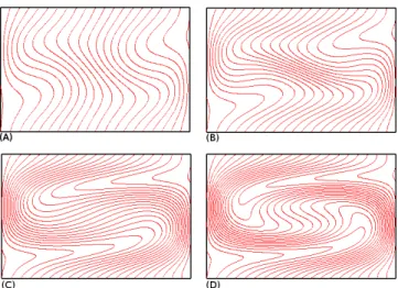
After the calculations are done, the program displays an animation of the changes in the magnetic field on the plasma as can be seen in Figure 1. This figure shows four different final states of PCell simulations after 100 time iterations with different parameter configurations.

C. OpenMP

Parallel processing has become common for achieving high performance. In the shared memory scheme, different pro-cessing units have asynchronous access to the same memory section in the computer for communication and data sharing. This kind of parallelism on often implemented with OpenMP (Open Multi-Processing) [13].

Fig. 1: PCell simulations of a magnetic fluid for different values of the Reynolds number (Rm) and plasma velocity (m): (a) Rm = 200, m = 0.1, (b) Rm = 500, m = 0.3, (c)Rm= 800, m= 0.7, (d) Rm= 1000, m= 0.9

parallelizes on athreadlevel within a process. In any OpenMP application there is a main thread that executes since the beginning of the program, once it reaches a section of the code that is to be parallelized, it spawns a specified number of slave threads that will all share a common memory space, the number of threads spawned can be set by environment variables or by code. These threads run concurrently and depend on the main thread that spawned them, the runtime environment assigns threads to different processing units.

Each one of the generated threads has an id which is an unique integer, and the master thread has an id of 0. After the parallel section of the code is executed, the threads merge back into the master thread, and the execution of the program is continued by it.

By default, each thread shares all of its memory with all the other threads, which means that if one of them changes the value of a variable, it changes it for all the other ones. OpenMP allows for variables to be declared private so that each thread can have its own local and independent variable so that any operation done by other threads on those variables doesn’t disrupt the others’. This is particularly important when calculations are being done concurrently and each thread will generate a different value, for example when dividing the workload of calculations done on an array or a matrix.

OpenMP is very popular and has been implemented in many compilers as well as several profilers and debuggers that support it. Among the C compilers that implement it are: GCC (GNU compiler), ICC (Intel compiler), and IBM XL.

III. PARALLELIZING THE SPATIAL DOMAIN

After running a profiler (gprof) on the sequential program, we discovered that the calculation of the convection function consumed 91.94% of the total execution time. One of the biggest loops within this function is the one that calculates the induction Equation (2), since it needs to iterate over every

point on the spatial grid four times (a fourth-order differential scheme).

On each temporal step of the simulation, a grid of spatial points is defined. For every one of these points the induction equation is calculated based on the state of the plasma in the previous time step, except for the first time step. This means there is a temporal dependency, since every calculation depends on the previous one, but there is no spatial dependence within a single time step so we were able to parallelize the spatial calculations on each point with OpenMP. After analyzing this section of the code, it was found that it is an embarrassingly parallel problem since no synchronization is needed for these operations and there is no dependency among them.

As can be seen in theconvectfunction shown in Algorithm 1, the main part of the program consists in four for loops. The two internal loops of the function (which are the ones that iterate in the spatial dimensions) are independent from each other. This makes these loops embarrassingly parallel, since there is no functional or data dependency between iterations. We divided the spatial grid among the available threads so that the calculations can be done simultaneously with OpenMP’s parallel for. We added the“parallel for”compiler directives on the loops that iterate through the grid so that the workload of the cycles is shared among the spawned threads. Most of the variables used in this part of the program had to be set as private so that each thread has its own copy since most of them were used to store intermediate values for the final calculation of the induction equation result on each grid point and if they are not declared private for each thread, the threads will share that memory space and the values would be overwritten or the threads could read values from another one, thus getting an incorrect value.

IV. EXPERIMENTS

A. Hardware setup

All the tests were performed at the Kabr´e supercomputer, an Intel Xeon Phi KNL node was used. This processor is highly configurable. It has 64 cores @ 1.3 GHz and 96 GB RAM. Each core has an L1 cache and pairs of cores are organized into tiles with a slice of the L2 cache symmetrically shared among them. All L2 caches among tiles are connected to the ones adjacent to it in a grid-like manner, each vertical and horizontal link is a bidirectional ring between them.

In order to maintain cache coherency, KNL has a distributed tag directory (DTD), organized as a set of per-tile tag di-rectories. Each one identifies the state and location of any cache line. A hash function is used to identify the directory responsible for a memory address.

Algorithm 1 convect function

Require: reyn: Magnetic Reynolds number

Require: m: field velocity parameter

Require: Tlim: time dimension parameter

Require: Xlim: x dimension parameter

Require: Ylim: y dimension parameter

Require: a: 3D array that holds the values of previous and current calculations

Require: vx: calculation of the stream motion function for the X dimension, array

Require: vy: calculation of the stream motion function for the Y dimension, array

potinc() 2: dx := 1/Xlim

dy := 1/Ylim 4: dt := 1/Tlim

re := 1/reyn 6: ex := dt/dx*12

ye := dt/dy*12 8: l := re*dt/(dx*dx)

m := re*dt/(dy*dy) 10: fort := 1 to Tlimdo

forn := 0 to 4do

12: forx := 0 to Xlimdo fory := 0 to Ylimdo

14: fa := 0

forcan := 1 to 2 do

16: ifcan == 1then

s := -1

18: z := 1

else

20: s := 1

z := 0

22: end if

ca:=−s∗ex∗(vx[x+s][y]∗(a[n+ 1][x+s][y]∗8

−a[n+z][x−2][y]) + (a[n+ 1][x+s][y+ 2]

−a[n+ 1][x+s][y−2])∗(vx[x+s][y+ 2]

−vx[x+s][y−2])/8

24:

cb:=−s∗ye∗(vy[x][y+s]∗(a[n+ 1][x][y+s]∗8

−a[n+z][x][y−2]) + (a[n+ 1][x+ 2][y+s]

−a[n+ 1][x−2][y+s])∗(vy[x+ 2][y+s]

−vy[x−2][y+s])/8

f a:=f a+ca+cb 26:

cc:=l∗(a[n+ 1][x+ 1][y] +a[n+ 1][x−1][y])+

m∗(a[n+ 1][x][y+ 1] +a[n+ 1][x][y−1])

Algorithm 1 convect function (continued)

cd:= 1−(ex∗vx[x+s][y]

+ye∗vy[x][y+s]) +s∗(l+m)

28: f e:=f a+cc

f i:=f e+a[n][x][y]∗cd 30: a[n+ 2][x][y] :=f i/cd

end for

32: end for

end for

34: end for end for

We configured our KNL in quadrant clustering mode. In this mode the tiles are divided into four parts called quadrants, which are spatially local to four groups of memory controllers. Memory addresses served by a memory controller in a quad-rant are guaquad-ranteed to be mapped only to directories contained in that quadrant.

B. Experiments description

Before parallelizing, we improved several aspects of the original program. We removed some redundant loops and cleaned up unnecessary variables. PCell was originally partly written in Fortran and translated with f2c [14], which is a program that automatically translates Fortran code to C. This automatic translation generated some of the issues mentioned previously.

After the initial improvements to the original program were made we integrated OpenMP into it, we ran this new version in our Xeon Phi nodes. We performed three different experiments to measure different variables, though some of the values used remained constant through all the experiments. The variables that did not change in any experiment were the magnetic Reynolds number, the value used was 800, and the velocity field parameter, the value used was 0.25. These parameters were chosen based on average values usually used for each one. For each test on every experiment, the program was executed 20 times on the same architecture to get a statistically relevant result.

1) Speedup experiment: For our first experiment we used as an independent variable the amount of OpenMP threads executing the program so we could measure the speedup obtained by gradually increasing them.

This test focused on the speedup obtained from adding threads to the execution. We tested the program with 1, 2, 4, 8, 16, 32, 64 and 128 threads. Each execution was done for a 500×500 spatial grid and 1000 time steps.

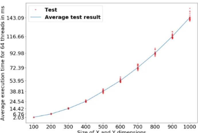
The program was tested with values from 100 × 100 to 1000 ×1000, with gradual increases of 100 for each dimen-sion. Notice that the size of the problem is being increased exponentially. This experiment was done with 64 threads and 1000 time steps.

3) Temporal scalability experiment: This experiment fo-cused on temporal scalability. It had as independent variable the amount of temporal iterations, which are the time-steps, in the simulation.

The program was tested with values from 1000 to 5000 with increments of 500. This experiment was done with 64 threads and 1000×1000 grid size.

V. RESULTS

A. Speedup

To measure the performance gain of the parallelized ver-sion of our application, we used the dimenver-sionless factor of speedup. After running the tests on our server, total execution time was taken for every run and then averaged, with this measure we could obtain speedup by dividing sequential time (Ts) by the averaged value of parallel time (Tp) we obtained from the tests as seen in Figure 2.

The data shows that the program scales in an almost linear way until we hit 128 threads. This is due to the fact that the Xeon Phi KNL processor has 64 physical cores. When using 128 threads we still get a little bit of speedup, but the growth with respect to speedup at 64 threads is not linear.

B. Spatial scalability

To measure scalability in performance for the spatial pa-rameters, we took the average execution walltime for every run. The results obtained can be seen in Figure 3.

The results have an exponential tendency, which is what is expected, since the grid size was increased in an exponential manner. Each dimension was increased by 100 between tests, and since the grid size is the result of the multiplication of the dimension sizes, the grid size increases exponentially.

The fact that the program scales this way means that we would be able to increase the size of the spatial matrix used in the simulation and the time it takes the computer to finish it would increase accordingly to the size of the input. This allows for larger spaces and a finer granularity to be achieved with the model. The original version of PCell did not allow for this increments to happen.

C. Temporal scalability

To measure scalability in performance for the temporal parameter, we took average execution walltime for every run. Figure 4 shows a quasi-linear scalability from the results, which indicates that the program scales linearly when increas-ing the temporal dimension of the simulation.

This improvement in scalability allows for longer simula-tions. If more time steps can be simulated with the model, we can use it to have a better understanding of the evolution of the phenomena that occur in plasma.

Fig. 2: Program Speedup. The max speedup obtained is just below 42×

Fig. 3: Scalability of spatial dimension increments

VI. CONCLUSIONS

We presented an OpenMP implementation of our fourth-order differential scheme for plasma simulation in fourth-order to improve its efficiency so that the simulations can cover wider spatial and temporal domains. The results show that our parallelized code decreases the total execution time for the application and allows us to increase both the spatial granularity and the temporal domain of simulations.

These improvements mean we can have faster and more accurate simulations, which will help to study different phe-nomena in plasma. This can for example help us study physical processes like magnetic reconnection in larger and more detailed areas over larger periods of time.

VII. FUTURE WORK

As for future work, we intend to further improve the performance of the simulation through MPI. The combination of MPI with OpenMP will help us accelerate the calculations when running the program on a cluster computer. This will allow us to increase the temporal and spatial granularity of the simulations to get more precise simulations. We will also be able to increase the size of the simulation so that it can be done on bigger areas or larger amounts of time as well as getting results on a shorter amount of time.

We also intend to explore better parallelization strategies based on the architecture that we have in our lab. We would like to test for better ways to exploit the vectorization capa-bilities of the KNL architecture.

ACKNOWLEDGMENTS

This research was partially supported by a machine alloca-tion on Kabr´e supercomputer at the Costa Rica Naalloca-tional High Technology Center.

REFERENCES

[1] C. Birdsall and A. Langdon,Plasma Physics via Computer Simulation, ser. Series in Plasma Physics and Fluid Dynamics. Taylor & Francis, 2004. [Online]. Available:https://books.google.co.cr/books?id= S2lqgDTm6a4C

[2] P. R. R.J Goldston,Introduction to Plasma Physics, 1995, vol. 19, no. 1. [3] P. V. Foukal, Solar Astrophysics, P. V. Foukal, Ed. Weinheim, Germany: Wiley-VCH Verlag GmbH, feb 2004. [Online]. Available: http://doi.wiley.com/10.1002/9783527602551

[4] R. Carboni and F. Frutos-Alfaro, “Computer simulation of convective plasma cells,” Journal of Atmospheric and Solar-Terrestrial Physics, vol. 67, no. 17-18 SPEC. ISS., pp. 1809–1814, 2005.

[5] K. Komatsu, R. Egawa, H. Takizawa, and H. Kobayashi, “Sustained Simulation Performance 2014,” 2015. [Online]. Available: http: //link.springer.com/10.1007/978-3-319-10626-7

[6] D.-J. Galloway and N. Weiss, “Convection and magnetic fields in stars,”

Astrophysical Journal, vol. 243, pp. 945–953, 1981.

[7] J. P. Verboncoeur, “Particle simulation of plasmas: review and advances,”

Plasma Physics and Controlled Fusion, vol. 47, no. 5A, p. A231, 2005. [Online]. Available:http://stacks.iop.org/0741-3335/47/i=5A/a=017 [8] R´emi Sentis,Mathematical Models and Methods for Plasma Physics,

Volume 1: Fluid Models. Birkh¨auser Basel, 2014, vol. 1.

[9] A. Ekenb, “MHD Modeling of the Interaction Between the Solar Wind and Solar System Objects,” pp. 554–562, 2005.

[10] P. A. Zegeling, “On Resistive MHD Models with Adaptive Moving Meshes,” Journal of Scientific Computing, vol. 24, no. 2, pp. 263– 284, aug 2005. [Online]. Available: http://link.springer.com/10.1007/ s10915-004-4618-6

[11] P. A. Davidson,An Introduction to Magnetohydrodynamics. Cambridge University Press, 2001.

[12] R. Carboni and F. Frutos-Alfaro, “Computer Simulation of Convective Plasma Cells,” pp. 1–18, 2015.

[13] OpenMP Architecture Review Board, “The OpenMP API specification for parallel programming,” 2015. [Online]. Available: http://www. openmp.org/wp-content/uploads/openmp-4.5.pdf