"Development of Multivariate Biomarker Genes as a Profile Predictor of Recurrence in Breast Cancer Patients" Edición Única

Texto completo

(1)

(2) INSTITUTO TECNOLÓGIC0 Y DE ESTUDIOS SUPERIORES DE MONTERREY CAMPUS MONTERREY ESCUELA DE BIOTECNOLOGÍA Y ALIMENTOS PROGRAMA DE GRADUADOS EN BIOTECNOLOGÍA. TEC de Monterrey DEL SISTEMA TECNOLÓGICO DE MONTERREY. " D E V E L O P M E N T O F MULTIVARIATE BIOMARKER G E N E S A S A PROFILE PREDICTOR OF R E C U R R E N C E IN BREAST C A N C E R PATIENTS''. TESIS PRESENTADA COMO REQUISITO PARCIAL PARA OBTENER EL GRADO ACADÉMICO DE: MAESTRO EN CIENCIAS CON ESPECIALIDAD EN BIOTECNOLOGÍA POR: RAFAEL JULIÁN CHACOLLA HUARINGA MONTERREY, N. L.. MAYO DE 2011.

(3) INSTITUTO TECNOLÓGICO Y DE ESTUDIOS SUPERIORES DE MONTERREY CAMPUS MONTERREY E S C U E L A DE BIOTECNOLOGIA Y ALIMENTOS P R O G R A M A DE G R A D U A D O S EN BIOTECNOLOGIA. TEC de Monterrey DEL SISTEMA TECNOLÓGICO DE MONTERREY. "Development of multivariate biomarker genes as a profile predictor of recurrence in breast cancer patients". TESIS P R E S E N T A D A COMO REQUISITO PARCIAL P A R A O B T E N E R E L GRADO ACADÉMICO DE:. M A E S T R O EN CIENCIAS C O N ESPECIALIDAD EN BIOTECNOLOGÍA. POR: R A F A E L JULIÁN C H A C O L L A HUARINGA. MONTERREY, N.L. a. MAYO DE. 2011.

(4) INSTITUTO TECNOLÓGICO Y D E ESTUDIOS SUPERIORES D E M O N T E R R E Y. CAMPUS MONTERREY E S C U E L A DE BIOTECNOLOGÍA Y ALIMENTOS P R O G R A M A DE GRADUADOS EN BIOTECNOLOGÍA. Los miembros del comité de tesis recomendamos que el presente proyecto de tesis presentado por el T M Rafael Julián Chacolla Huaringa, sea aceptado como requisito parcial para obtener el grado académico de:. Maestro en Ciencias con Especialidad en Biotecnología Comité de Tesis:. Dr. Sean Patrick Scott Sartini Co-Asesor. Dr. Víctor Manuel Treviño Alvarado Co-Asesor. Dr. Servando Cardona Huerta Sinodal. Aprobado:. Dr. Jorge Welti Chanes Director de Posgrado de la Escuela de Biotecnología y Alimentos Mayo 2011.

(5) ACKNOWLEDGMENTS. I am infinitely grateful for the aid o f genteel people such as workers and professors for their academic services from Instituto Tecnológico y de Estudios Superiores de Monterrey and C O N A C y T for their financial support that have made things possible. I would like to thank so many people that it is impossible to find any order for their respective contributions. Let's start: Dr. Jose Rafael Borbolla for his kind invitation to join to the Cátedra de Hematología y Cancer at I T E S M as master's student. He followed me since initiated o f the master studies and has made possible accomplish some challenges in my life. I thank him for his infinite and invaluable confidence during these years. Dr. Sean Scott and Victor Trevino for their support as advisors o f this current thesis, their help was invaluable for my research. M y colleagues belong to Bioinformatics Group at the I T E S M . I have passed great moments with them during the last year o f research. M y mom and dad Celia Huaringa and Julián Chacolla for their love, support, sacrifice and positive influences. I have a special thanks to my brother William, because he is always an ideal image to follow. M y friends from Peru are a great motivation every day and I thank them for their advices to never to give up on this adventure and keep walking for my dreams. I also thank my friends from Europe and Asia for their support and positive influences since I met them. Finally, all my teachers who have opened my mind to such interesting research fields..

(6) CONTENTS 1. Introduction 1.1 Breast Cancer Recurrence. 1 2. 1.1.1. Local Recurrence. 2. 1.1.2. Regional Recurrence. 3. 1.1.3. Distant Recurrence. 3. 1.2 Research Objectives. 4. 1.2.1 General Objectives. 4. 1.2.2 Specific Objectives. 4. 2. State of the Art. 5. 2.1 Some signatures can predict different stages of breast cancer. 5. 2.2 Finding biomarkers to predict recurrence breast cancer. 7. 2.3 Microarray Databases. 7. 2.4 Meta-analysis. 8. 2.5 Biomarker discovery. 10. 2.6 Survival analysis. 11. 2.6.1. Censoring data. 12. 2.6.2. Analysis o f recurrence data using hazard function. 13. 2.6.3. C o x Proportional Hazards Model Formulation. 14. 2.6.4. Feature Selection. 16. 2.6.5. Multivariate analysis o f microarray data. 17. 3. Materials and methods 3.1 Methodology to develop multivariate biomarker genes. 19 19. 3.1.1. Data Collection and Merging. 20. 3.1.2. Pre-processing microarray data. 23.

(7) 3.1.3. Cox univariate model. 27. 3.1.4. Multivariate analysis by PSO. 28. 3.1.5. Model building. 30. 3.1.6. Model assessment. 30. 3.2 Validation by real time PCR. 33. 3.2.1. Clinical Information of patients. 33. 3.2.2. Validation of the multivariate biomarker genes by real time PCR. 34. 4. Results and Discussions. 38. 4.1 Pre-processing microarray data genes. 39. 4.2 Univariate analysis. 41. 4.3 Cox multivariate analysis. 43. 4.4 Model Building. 46. 4.5 Accuracy assessment. 51. 4.6 Validation in R T - P C R. 59. 4.6.1. Standard curve of G A P D H. 62. 4.6.2. Standard curve of AP2B1. 63. 4.6.3. Standard curve of SF3B3. 64. 4.6.4. Standard curve of R R M 2. 65. 4.6.5. Standard curve of PPFIA1. 66. 4.6.6. Standard curve of C13orf35. 67. 4.6.7. Standard curve of VPS41. 68. 4.6.8. Standard curve of R A C G A P 1. 69. 4.6.9. Standard curve of GPR56. 70. 5. Conclusions. 77. 6. Bibliography. 79.

(8) List of Figures Figure 2.1: Gene expression prognostic and predictive classifiers. 6. Figure 2.2: Cancer gene expression profiling with microarray experiments. 9. Figure 2.3: Meta-analysis. Collection o f datasets from different research laboratories are merged in one huge dataset 10 Figure 2.4: Occurrence and timing o f an event. It is studied by the time between start state and end state 12 Figure 2.5: Censoring situations. 13. Figure 3.1: Flow-chart o f the methodology proposed to develop robust biomarker genes. 20 Figure 3.2: M A S 5 . 0 Background correction. 24. Figure 3.3: After quantile normalization. 25. Figure 3.4: Example o f hierarchical representation (dendrogram) produced by a hierarchical clustering analysis o f 7 patients 26 Figure 3.5: Illustrates the use o f a heatmap in combination with hierarchical clustering in order to visualize the gene expression 26 Figure 3.6: Home page o f Biom@tec. 27. Figure 3.7: Schematic representation o f Hazard function used as C o x univariate model... 27 Figure 3.8: It illustrates the beginning o f univariate analysis by C o x regression model per gene 28 Figure 3.9: Schematic representation o f Particle Swarm Optimization (PSO). 29. Figure 3.10: This illustrates the performed risk score in all patients o f meta-dataset, it can be then divided in low and high risk groups 30 Figure 3.11: Schematic representation o f statistical phase to find multivariate biomarker genes 32 Figure 4.1: Normalization. 39.

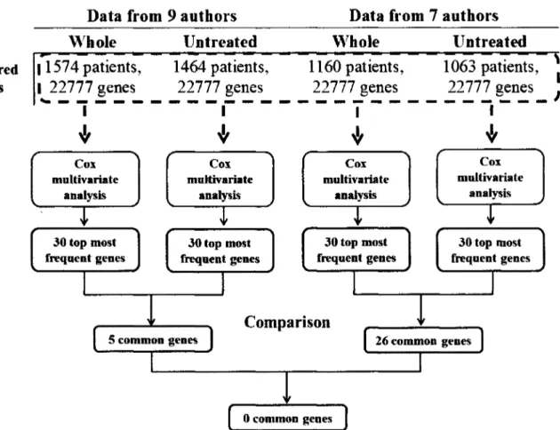
(9) Figure 4.2: Hierarchical clustering of meta-data after normalization. 40. Figure 4.3: Hierarchical Clustering of meta-dataset after adjustment. 41. Figure 4.4: Box plot diagram of different model sizes, top of the figure illustrates the correlation of increase size model according with increase of the overfitting. 44. Figure 4.5: Comparison o f three different sets of data to start the multivariate analysis.... 47 Figure 4.6: Schematic representation of methodology applied to eight sizes o f data to generate robust biomarker genes 48 Figure 4.7: Schematic representation of first part methodology applied to 4 eight sizes of data to generate robust biomarker genes 49 Figure 4.8: Schematic representation of second part methodology applied to 4 eight sizes o f data to generate robust biomarker genes 50 Figure 4.9: Schematic representation of final comparison o f two last results, and building o f basic model with four genes 51 Figure 4.10: Assessment of four multivariate biomarker genes. 52. Figure 4.11: Schematic representation of methodology used to find 6 six genes to complete the model of 10 genes 53 Figure 4.12: Assessment of ten multivariate biomarker genes in whole data from nine authors 55 Figure 4.13: Assessment of ten multivariate biomarker genes in patients without treatment before surgery from nine authors 56 Figure 4.14: Assessment of ten multivariate biomarker genes in patients with treatment before surgery 57 Figure 4.15: Schematic methodology to make standard curve. It was a subsequent five serial dilutions since 20 to 0.0002ng/ul 60 Figure 4.16: Schematic methodology to make standard curve. It was a subsequent five serial dilutions since 2 to 0.00002ng/ul 61 Figure 4.17 Standardization of G A P D H. 62. Figure 4.18: Standardization of AP2B1. 63. Figure 4.19: Standardization of SB3F3. 64. Figure 4.20: Standardization of R R M 2. 65. Figure 4.21: Standardization of PPFIA1. 66. Figure 4.22: Standardization of C13orf35. 67.

(10) Figure 4.23: Standardization of VPS41. 68. Figure 4.24: Standardization of R A C G A P 1. 69. Figure 4.25: Standardization of GPR56. 70. Figure 4.26: Assessment of eight multivariate biomarker genes in whole data from nine authors 72.

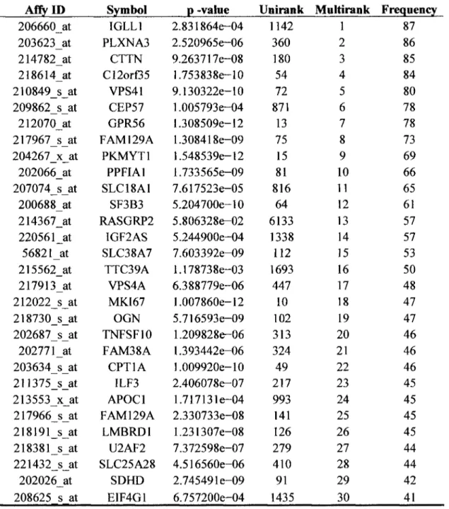
(11) List of Tables Table 2.1: List o f selected databases with publicly available breast cancer microarray data, modified from Cheang et al. 2008. 8. Table 3.1: Nine datasets downloaded from G E O Database with respectively amount o f patients 21 Table 3.2: Clinical marker status. 22. Table 3.3: Clinical treatment information pre-surgery. 22. Table 3.4: Clinical treatment information post-surgery. 23. Table 3.5: Clinical information o f patients, this illustrates in detail each clinical item o f patients. 34. Table 3.6: Set up o f genomic D N A elimination reaction. 35. Table 3.7: Set up reverse transcription reaction. 35. Table 3.8: It illustrates the sequences o f 10 set o f primers o f the multivariate biomarker genes and 1 set o f primers o f the housekeeping gene 36 Table 3.9: Set up the real time P C R reaction. 37. Table 3.10 Real-time cycler conditions. 37. Table 4.1: It illustrates 20 significant genes with their symbol gene, p-value and q-value sorted by lowest p-values 42 Table 4.2: It illustrates the 30 most frequent genes involved in 1000 models generated.... 45 Table 4.3: It illustrates eight sizes of data tested by Cox multivariate analysis. 48. Table 4.4: It illustrates the ten multivariate biomarker genes chosen to predict recurrence in breast cancer patients, and the biological function o f them involved 54 Table 4.5: Results summary o f statistical parameters used in assessment o f set o f ten multivariate biomarker genes. 58. Table 4.6: It illustrates the reaction setup. 59. Table 4.7: It illustrates the reaction setup. 60.

(12) Table 4.8: Numerical data from standard curve of G A P D H. 62. Table 4.9: Numerical data from standard curve of AP2B1. 63. Table 4.10: Numerical data from standard curve of SF3B3. 64. Table 4.11: Numerical data from standard curve of R R M 2. 65. Table 4.12: Numerical data from standard curve of PPF1A1. 66. Table 4.13: Numerical data from standard curve of C12orf35. 67. Table 4.14: Numerical data from standard curve of VPS41. 68. Table 4.15: Numerical data from standard curve of R A C G A P 1. 69. Table 4.16: Numerical data from standard curve of GPR56. 70. Table 4.17: Statistical differences between results used in assessment from set of ten and eight multivariate biomarker genes using whole data of 9 datasets 71 Table 4.18: C T values o f each gene for ten breast cancer samples. 73. Table 4.19: Data normalized by reference gene expression, this table also shows the mean and standard deviation (SD) for each gene tested 73 Table 4.20: It illustrates the mean and S D from Affymetrix dataset used in meta-analysis foe each gene 74 Table 4.21: It illustrates the transformed values to reach a similar mean and SD values... 74 Table 4.22: It illustrates the prognostic index for each gene in samples. 75. Table 4.23: It illustrates the ten patients tested with their respectively prognostic index values and their risk to develop recurrence. 76.

(13) D E V E L O P M E N T OF M U L T I V A R I A T E B I O M A R K E R GENES A S A PROFILE P R E D I C T O R OF R E C U R R E N C E I N B R E A S T C A N C E R P A T I E N T S. 2011. CHAPTER 1. INTRODUCTION. Breast cancer is the most commonly diagnosed cancer and the leading cause o f cancerrelated death among women worldwide, with more than 800,000 new cases o f breast cancer diagnosed annually, representing 2 1 % o f all new cancers in women. Additionally, globally estimates suggest the highest age-adjusted breast cancer incidence rate is reported for North America, including Mexico, at 99.4 new cases per 100,000 women per year. Breast cancer accounts for nearly one in every three cancers diagnosed among women in the U . S . (Bird et al, 2010). In the contemporary management o f breast cancer, several possibilities exist for local and regional treatment. Patients and their oncologists must decide between various surgical options and the dose, volume, and technique o f radiotherapy. These decisions may have a significant impact on treatment-related morbidity and survival from breast cancer (Voduc et al. 2010). The primary treatment o f localized breast cancer is either complete tumour excision and radiation or mastectomy with or without radiotherapy. The addition o f systemic adjuvant therapies (chemo, endocrine and/or trastuzumab), which are designed to control micrometastatic disease, to the primary treatment o f localized breast cancer has been shown to increase the chance o f long-term survival (Colozza et al. 2006). In recent years, breast conserving surgery followed by radiotherapy is accepted as a standard treatment for many patients with early-stage breast cancer. In appropriately selected cases, it is known to result in equivalent survival to mastectomy with high rates o f local control. Local failure does present a problem in a significant minority o f patients, with breast cancer INSTITUTO TECNOLOGICO Y DE ESTUDIOS SUPERIORES DE MONTERREY. Page 1.

(14) D E V E L O P M E N T OF M U L T I V A R I A T E B I O M A R K E R G E N E S A S A P R O F I L E PREDICTOR OF R E C U R R E N C E IN B R E A S T C A N C E R PATIENTS. 2011. recurrence rates o f 5-10% at 5years following initial treatment and 7-18% at 10 years (McBean et al. 2003). The biological significance o f breast recurrence on the subsequent course o f the disease is disputed, with conflicting results published. Some studies (Elkhuizen et al. 1998). suggest that breast recurrence heralds the development o f distant metastases and has a significant adverse effect on survival, while others (Moran and Haffty, 2002) that patients with an operable recurrence can be successfully salvaged. The clinician is faced with the patient with the practical problem o f recurrence in the treated breast requires guidance for subsequent management. Data from randomized controlled trials are not available, and therefore reviews o f databases or retrospective surveys are the only sources on which to base management decisions. Various clinical and pathological factors, such as age, menopausal status, tumour size, histological grade, lymphovascular invasion, estrogen receptor (ER) and E R B B 2 receptor status, have been carefully evaluated as prognostic indicators o f clinical course. Most o f these variables are combined into prediction models such as the Nottingham Prognostic Index (NPI) and Adjuvant!Online, or included in algorithms used for the development o f guidelines for treatment decision-making (Sotiriou and Piccart, 2007).. 1.1 Breast Cancer Recurrence Recurrence o f breast cancer after definitive local treatment poses a challenging problem for the treating physicians. The definition o f recurrence describes the return o f breast cancer after primary treatment. There are three types o f recurrent breast cancer: 1.1.1 L o c a l recurrence It occurs when cancerous cells reappear at the original tumour site over time. Local breast cancer recurrence is not considered to be a spread o f the cancer but rather due to failure o f the initial treatment. Even after mastectomy, portions o f breast skin and fat remain, making local recurrence possible, albeit uncommon. Rather, it is women treated with breast-conserving therapy and radiation who are at slightly higher risk o f this type o f recurrence. Treatment o f locally recurring breast cancer depends on the initial therapy undertaken at the time o f first. INSTITUTO TECNOLOGICO Y DE ESTUDIOS SUPERIORES DE MONTERREY. Page 2.

(15) D E V E L O P M E N T OF M U L T I V A R I A T E B I O M A R K E R GENES A S A PROFILE PREDICTOR OF R E C U R R E N C E IN B R E A S T C A N C E R PATIENTS. 2011. diagnosis. I f breast conserving surgery was originally performed, recurrent breast cancer w i l l usually be treated with mastectomy (Kurtz et al, 1989,). 1.1.2 Regional recurrence It is more serious than local recurrence because it usually indicates that the cancer has spread past the breast and underarm (auxiliary) lymph nodes. Regional recurrences o f breast cancer can occur in the chest muscles, in the internal mammary lymph nodes under the breastbone and between the ribs, in the nodes above the collarbone and in the nodes surrounding the neck. The latter two sites o f regional recurrence tend to suggest more aggressive cancers. Overall, regional recurrence is very common, occurring in approximately 2% - 5% o f all breast cancer cases. Treatment can be complex however, including surgery to remove the cancerous node, radiotherapy, chemotherapy and adjuvant endocrine therapy depending on the previous treatment used (Haffty et al. 1990). 1.1.3 Distant recurrence It also known as metastasis, it is the most serious type o f recurrence and is associated with significantly lower survival. Having left the confines o f the breast tissue, the cancer usually spreads first to the axillary lymph nodes. In 65-75% o f distant recurrences the breast cancer then spreads from the lymph nodes to the bone. More rarely, the breast cancer may metastasize to other sites including the lungs, liver, brain or other organs. Surgery is rarely an option for metastatic breast cancer because the cancer is not usually confined to one specific site on a given organ. Instead, treatment approaches include chemotherapy, radiation therapy or endocrine therapy (Joensuu et al. 2004). Numerous studies have attempted to identify prognostic factors after local-regional failure and to assess the risk o f distant spread. Currently, one o f the most important and urgent clinical questions in breast cancer recurrence is how we can avoid it, and identify the subset o f patients who can be safely spared adjuvant chemotherapy among different clinical profiles as lymph node negative or positive, different progression grades and estrogen receptor negative or positive from breast cancer patients. Furthermore these patients could show a relatively favorable or adverse prognosis when treated with adjuvant hormonal therapy alone. In order to reduce the. INSTITUTO TECNOLOGICO Y DE ESTUDIOS SUPERIORES DE MONTERREY. Page 3.

(16) D E V E L O P M E N T OF M U L T I V A R I A T E B I O M A R K E R GENES A S A PROFILE PREDICTOR OF R E C U R R E N C E IN B R E A S T C A N C E R PATIENTS. 2011. recurrence rate, most o f such patients are currently treated with not only adjuvant hormonal therapy but also adjuvant chemotherapy even though adjuvant chemotherapy is considered to be unnecessary for the majority. It can therefore be said to be o f vital importance the search o f biomarker that can predict the prognosis o f such patients with high accuracy and to administer adjuvant chemotherapy only to those who are at high risk o f recurrence.. 1.2 Research Objectives The present research project is based on statistical methodology to develop a set o f robust biomarker genes that can predict the prognosis o f breast cancer patients with high accuracy. 1.2.1 General Objective •. To develop a methodology to find a set o f multivariate biomarker genes as a significant profile predictor o f recurrence in breast cancer patients.. 1.2.2 Specific Objectives •. To find available microarray data that contains recurrence clinical information.. •. To perform the pre-processing o f microarray data.. •. To perform univariate analysis method.. •. To perform multivariate analysis method.. •. To evaluate results from univariate and multivariate analysis for building o f a model.. •. To assess the accuracy o f the built model to predict high and low risk in patients with breast cancer.. •. To validate the set o f biomarker genes in Mexican breast cancer patients by real time P C R experiments.. INSTITUTO TECNOLOGICO Y DE ESTUDIOS SUPERIORES DE MONTERREY. Page 4.

(17) D E V E L O P M E N T OF M U L T I V A R I A T E B I O M A R K E R GENES A S A PROFILE PREDICTOR OF R E C U R R E N C E IN B R E A S T C A N C E R PATIENTS. 2011. CHAPTER 2. STATE OF THE ART Development o f effective tools such as D N A microarrays for monitoring gene expression on a large scale has resulted in the discovery o f gene networks and regulatory pathways in various tumor processes (Trevino et al. 2007). In this respect, global gene expression in breast cancer has been profiled extensively over the last decade, which allowed the identification o f breast cancer molecular subtypes, stages and the development o f prognostic and predictive gene signatures, resulting in an improved understanding o f the heterogeneity o f breast cancer (Desmedt et al. 2009).. 2.1 Some signatures can predict different stages of breast cancer Microarray technology has led to the development o f important prognostic signatures that assist in predicting the risk o f recurrence in breast cancer patients. Gene expression profile o f primary breast tumors may be encoded by some genes driving recurrence. Transcriptomics analysis o f a variety o f primary tumors by Ramaswamy and colleagues in 2003 identified a 17gene signature present in a wide range o f human primary tumors which predicted metastasis and poor clinical outcome. V a n de Vijver in 2002 applied microarray technology to identify gene expression profile in primary breast tumors associated with early distant metastasis and poor survival. Recently, M i n n and colleagues in 2005 have identified a set o f genes which mediate breast cancer metastasis to the lung; expression was found to translate to decreased lungmetastasis-free survival in a cohort o f 82 patients. Nuyten and colleagues in 2006 demonstrated that the presence o f wound response gene expression signature identified patients at increased risk o f local recurrence.. INSTITUTO TECNOLOGICO Y DE ESTUDIOS SUPERIORES DE MONTERREY. Page 5.

(18) D E V E L O P M E N T OF M U L T I V A R I A T E B I O M A R K E R GENES AS A PROFILE P R E D I C T O R OF R E C U R R E N C E I N B R E A S T C A N C E R P A T I E N T S In breast cancer research to date, most studies focus on developing a gene expression prognostic and prediction classifier according with, respectively, clinical stage as shown in Figure 2.1; it is supported by several publications which focus to identify limited sets o f key genes within expression signatures (Cheang et al. 2008).. Figure 2.1: Gene expression prognostic and predictive classifiers. A) The prognostic classifier is generated using gene-expression data from tumour surgical specimens, and clinical outcome (development of recurrence during follow-up). B) The predictive classifiers of response to treatment are generated by correlating gene-expression data, derived from biopsies taken before pre-operative systemic therapy, with clinical and/or pathological response to the given treatment (b); modified from Sotiriou and Piccart, 2007. Commercially available assays based on gene expression profiling, including Oncotype D X (Genomic Health, Redwood City, C A ) and MammaPrint (Agendia, Amsterdam, the Netherlands), may provide useful prognostic information (Van de Vijver et al. 2002 and Paik et al. 2004). INSTITUTO TECNOLOGICO Y DE ESTUDIOS SUPERIORES DE MONTERREY. Page 6.

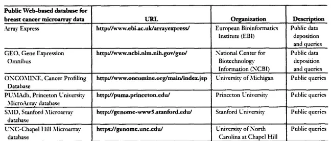
(19) D E V E L O P M E N T OF M U L T I V A R I A T E B I O M A R K E R GENES A S A PROFILE P R E D I C T O R OF R E C U R R E N C E I N B R E A S T C A N C E R P A T I E N T S. 2011. 2.2 Finding biomarkers to predict recurrence breast cancer Although most studies o f molecular subtypes in breast cancer report differences in survival, few have examined the differences in loco-regional recurrence. The influence of breast cancer molecular subtypes on loco-regional relapse and their relevance compared with established clinic-pathologic variables has not been defined (Voduc et al. 2010). Biomarker studies can provide prognostic information that may facilitate treatment decisions. The molecular biomarkers like expression o f estrogen and growth factor receptors, pS2, metallothionein, CD24, cathepsin D , E R B B 2 , and mutations in the TP53 gene all have been correlated to breast cancer prognosis (Esteva and Hortobagyi, 2004), the use o f single marker provides limited information for the prognosis o f an individual patient. In view o f the molecular heterogeneity o f breast tumors and the large number o f marker genes involved, studying multiple genetic alterations simultaneously is o f the utmost importance. With the arrival o f microarray technologies, searches for tumor markers can be performed in a discovery-driven manner in high through-put way.. 2.3 Microarray databases In the last years, enormous data has been generated with microarray experiments from different types o f cancer and platforms under various experimental conditions. Databases like the N C B I Gene Expression Omnibus ( G E O ) (Barrett et al. 2007), Oncomine (Rodhes et al. 2007), ArrayExpress (Parkinson et al. 2007) and N A S C A r r a y s (Craigon et al. 2004) have been set up to archive these datasets and to make them available to the scientific community. The size o f microarray databases is likely to increase exponentially in the future, as is typical for all molecular databases, increasing the need for sophisticated methods to analyze these large amounts o f data appropriately.. INSTITUTO TECNOLOGICO Y DE ESTUDIOS SUPERIORES DE MONTERREY. Page 7.

(20) D E V E L O P M E N T OF M U L T I V A R I A T E B I O M A R K E R GENES A S A PROFILE P R E D I C T O R OF R E C U R R E N C E I N B R E A S T C A N C E R P A T I E N T S. 2011. Public Web-based database for URL. breast cancer microarray data. Organization. Description. Array Express. http:ZAvww.ebi.ac.uk/arrayexpress/. European Bioinformatics Institute (EBI). Public data deposition and queries. G E O , Gene Expression. http://www.ncbi.nlm.nih.gov/geo/. Xational Center for. Public data deposition and queries. Biotechnology. Omnibus. Information (XCBI) O X C O M I X E , Cancer Profiling. http://www.oncomine.org/main/index.jsp. University of Michigan. Public queries. http://puma.princeton.edu/. Princeton University. Public queries. http://genome-wwwS.stanford.edu/. Stanford University. Public queries. https://genome.unc.edu/. University of Xorth Carolina at Chapel Hill. Public queries. Database PUAlAdb, Princeton University MicroArrav database SMD, Stanford Microarray database UXC-Chapel Hill Microarray database. Table 2.1: List of selected databases with publicly available breast cancer microarray data, modified from Cheang et al. 2008.. 2.4 Meta-Analysis With high-dimensional variables (thousands o f genes), microarray data suffer from small numbers o f samples and are often notorious for their low signal-to-noise ratio. However, microarray technologies are becoming more prevalent for cancer research, and it is now usual to find several gene expression data sets from different laboratories employing the same/different technologies to identify genes related to the same condition. Meta-analysis is a statistical technique for combining these quantitative findings from independent studies. Therefore, metaanalysis o f gene-profiling data is increasingly required to integrate data sets that investigate a common theme or disorder, and to yield more valid and informative results than each experiment separately (Yang and Sun, 2009). Several factors impede a straight-forward analysis o f microarray database content: standards for data submission vary between different databases, some microarray datasets do not provide raw data and on the experimental side, protocols and experimental conditions can differ between. different. laboratories conducting microarray hybridizations. However, a major. advantage o f microarray meta-analysis is that through the integration o f a potentially large number o f datasets, additional insights into gene regulation can be gained which could have been overseen or not detected in the single experiments. Reasons for this could be that either the signal from a particular gene or group o f genes was too weak to be detected in the single. INSTITUTO TECNOLOGICO Y DE ESTUDIOS SUPERIORES DE MONTERREY. Page 8.

(21) D E V E L O P M E N T OF M U L T I V A R I A T E B I O M A R K E R G E N E S A S A P R O F I L E P R E D I C T O R OF R E C U R R E N C E IN B R E A S T C A N C E R P A T I E N T S experiment or because it can be put into a functional context taking into consideration its regulation under other conditions or treatments (Ramasamy et al. 2009).. Figure 2.2: Cancer gene expression profiling with microarray experiments. Collection of gene expression profiles from several breast cancer tissues to make a dataset, modified from Rhodes et al. 2004.. The general assumption for meta-analysis is that many researches into one topic can be combined into a large study in terms o f "effect sizes." The effect size encodes the selected research findings (effects) on a numeric scale. It provides information regarding how much an expression change is evident either across all studies or for a subset o f studies. Two common strategies for modeling the effect size o f microarray include either transforming gene expression measures across studies or generating summaries such as p-values, probabilities, or ranks (Conlon et al. 2007). Several methods for microarray meta-analysis has been proposed in recent years, most o f them using models which compute an "effect size" and take care o f inter-study variation (Choi et al. 2003; Moreau et al. 2003). Thus, they often resemble procedures applied for the detection o f differential expression but add the study as an extra explanatory variable. Several datasets from different microarray experiments are integrated in the meta-analysis to increase the number o f replicates and thereby the power to detect differentially expressed genes as biomarkers (Engelmann et al. 2008). For this reason the methods used to process and evaluate datasets merged is crucial in the development o f a meta-analysis.. INSTITUTO TECNOLOGICO Y DE ESTUDIOS SUPERIORES DE MONTERREY. Page 9.

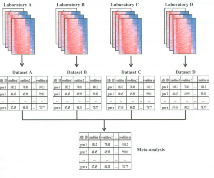
(22) D E V E L O P M E N T OF M U L T I V A R I A T E B I O M A R K E R G E N E S A S A P R O F I L E P R E D I C T O R OF R E C U R R E N C E IN B R E A S T C A N C E R P A T I E N T S. Figure 2.3: Meta-analysis. Collection of datasets from different research laboratories are merged in one huge dataset.. In the context o f gene expression analysis, biomarker discovery means identification o f an optimal subset o f variables (genes) that significantly differentiates the classes and can be used for accurate prediction o f the class membership (Dziuda, 2010). Although it may happen that a biomarker consists of just one variable, most often finding a good biomarker means searching for a set o f variables, which together as a set can separate the classes, (high or low risk to predict recurrence in breast cancer patients). The main goals o f biomarker discovery are:. INSTITUTO TECNOLOGICO Y DE ESTUDIOS SUPERIORES DE MONTERREY. Page 10.

(23) D E V E L O P M E N T OF M U L T I V A R I A T E B I O M A R K E R GENES A S A PROFILE P R E D I C T O R OF R E C U R R E N C E I N B R E A S T C A N C E R P A T I E N T S •. 2011. T o identify small subsets o f variables that can be used for the efficient classification o f new samples.. •. To provide fast and cost-effective classifiers that can be easily implemented into clinical practice.. •. To link the identified biomarkers and the class differences with underlying biological processes. Biomarker discovery has been applied to several medical research areas. The following. are just a few examples o f biomarker types: •. Diagnostic biomarkers indicate the presence o f a disease or the presence o f a specific state or subtype o f the disease.. •. Prediction biomarkers indicate the probability o f specific outcomes o f a treatment.. •. Biomarkers for personalized medicine (for instance, biomarkers for therapy selection or for minimizing the risk o f adverse drug reactions) indicate the probability o f a specific outcome for the considered therapy options or medications. The specific therapy to the condition o f a patient is important in cancer treatment. Over-. treatment o f patients that have a low risk o f recurrence may cause therapy induced conditions, such as leukemia. Although there are some types o f treatment protocols for breast cancer patients, there are still significant challenges in predicting which o f available treatment options will be most appropriate for a particular breast cancer patient. For this reason the search o f biomarkers using microarray data that can predict which patient belong either groups o f low or high risk, it is a challenge in the current personalized medicine.. 2.6 Survival Analysis Survival analysis is a class o f statistical methods for studying the occurrence and timing of events. These methods are most often applied to the study o f deaths but can treat different kind o f events including the onset o f disease, equipment failures, recurrence, etc.. INSTITUTO TECN0L0GICO Y DE ESTUDIOS SUPERIORES DE MONTERREY. Page 11.

(24) D E V E L O P M E N T OF M U L T I V A R I A T E B I O M A R K E R GENES A S A PROFILE P R E D I C T O R OF R E C U R R E N C E I N B R E A S T C A N C E R P A T I E N T S. 2011. Survival analysis was designed for longitudinal data on the occurrence o f events. A n event can be defined as a qualitative change that can be situated in time. For instance a disease consists o f a transition from a healthy state to a diseased state.. Outcome variable: Time until an event occurs. Figure 2.4: Occurrence and timing of an event It is studied by the time between start state and end state.. Moreover, the timing o f the event is also considered for analysis. Ideally, the transitions occur virtually instantaneously and the exact time at which the event occurs is known. Some transitions may take a little time, however, and the exact time o f onset may be unknown or ambiguous. For survival analysis, the best observation plan is prospective. B y prospective we mean that the observation o f a set o f individuals starts at some well-defined point in time and they are followed for some substantial period o f time, recording the time at which the events o f interest occur. 2.6.1 Censoring data Censored data occurs when you know that a measurement exceeds some threshold, but you don't know by how much, but there is a less common kind o f censored data where you know that a measurement falls below some threshold, but do not know by how much. Both common situations are depicted in Figure 2.5.. INSTITUTO TECNOLOGICO Y DE ESTUDIOS SUPERIORES DE MONTERREY. Page 12.

(25) D E V E L O P M E N T OF M U L T I V A R I A T E B I O M A R K E R G E N E S A S A P R O F I L E PREDICTOR OF R E C U R R E N C E IN B R E A S T C A N C E R PATIENTS. 2011. Figure 2.5: Censoring situations. The "X" symbols represent the points in time when the experiments start or finish monitoring the censored entities. Line (A) shows an entity that has already been "operating" for some unknown period of time, before we start monitoring it. This case is called "left-censoring". Line (B) shows an entity that has been monitored since the beginning of the experiment, but I was not followed until the end of the experiment (time To). This case is called "right-censoring". The entity in Line (C) has been monitored all along the experiment.. 2.6.2 Analysis of recurrence data using hazard function A n aspect o f analysis o f survival time data that has gained popularity, especially in medical research is assessing the relationship between outcome time and some biological expression data found in genomics, proteomics, metabolomics and transcriptomics areas that could possibly affect the outcome status o f patients. Recurrence data can explore how the recurrence experience o f a group o f patients depends o f the values o f one or more explanatory variables (in this case: expression o f genes), whose values have been recorded for each patient at the time origin. Due to censoring, standard linear regression methods are not feasible in modeling such relationship. One popular regression model formulation that is often used in survival analysis is the C o x (1972) proportional hazards model. The model utilizes the hazard function h{t), that specifies the instantaneous rate o f failure at T = / conditional upon survival to time t. The model (2.1) is defined as the probability o f experiencing event o f failure in the infinitesimally small interval (/, /+A/), given that such an event has not been experienced prior to t. It is expressed as:. INSTITUTO TECNOLOGICO Y DE ESTUDIOS SUPER10RES DE MONTERREY. Page 13.

(26) D E V E L O P M E N T OF M U L T I V A R I A T E B I O M A R K E R GENES A S A PROFILE PREDICTOR OF R E C U R R E N C E IN BREAST C A N C E R PATIENTS. 2011. (2.1). The probability in the numerator is conditional on the individual surviving to time t because individuals who have already experienced the event should not be considered.. 2.6.3 Cox Proportional Hazards Model Formulation. Cox (1972) made two significant innovations. First, he proposed a model that is standardly referred as the proportional hazards model. Second, he proposed a new estimation method that was later named maximum partial likelihood. The term C o x regression refers to the combination of the model and the estimation method.. The Model: Consider failure times T ,T ,...,T x. values x ,x ,...,x n. j2. 2. n. o f n individuals. For each individual / we have. o f k explanatory variables. Note that the explanatory may include both. ik. quantitative variables and qualitative variables such as treatment group, the latter can be incorporated through the use o f indicator variables. The principal problem dealt with in this section is that o f modeling the relationship between the failure time T and explanatory variables. The exponential distribution can be generalized to obtain a regression model by allowing the failure rate o f 7] to be function ofx ,x ,...,x . In regression models it is common practice that n. J2. jk. the dependent variable depends on the explanatory variables only through a linear function. P x + fi x +... + P x x. a. 2. where P ,p p ,...,fi. l2. Q. v. 2. k. k. lk. ,. (2.2). are unknown parameters. According the formulation's Collet (1993) in a. regression model for survival analysis one can try to model the dependence on the explanatory by taking the (new) hazard rate, then modeled by. h{t) = \ it) x espip. lXn. + P x +... + p x ), 2. l2. k. lk. INSTITUTO TECNOLOGICO Y DE ESTUDIOS SUPERIORES DE MONTERREY. (2.3). Page 14.

(27) D E V E L O P M E N T OF M U L T I V A R I A T E B I O M A R K E R GENES A S A PROFILE P R E D I C T O R OF R E C U R R E N C E I N B R E A S T C A N C E R P A T I E N T S The. model x. exp (/?,*,, + P a 2. (2.3). is x. +••• + Pk ik). semi-parametric l s. because. the. 2011. dependence. function. modeled explicitly but no specific probability distribution is. assumed for the survival times. Thus /? is only estimable through the partial likelihood estimation procedure.. The assumption o f no tied events, gave the partial likelihood function as. (2.4). where. R(Us)),. the risk set at. t$). as the set o f all individuals who are still under study at the time. just prior to fy),and the log partial likelihood as. (2.5). Often, ties occur in continuous survival data that are collected in days, weeks and months (Collett, 1993). When there are only a few ties, Breslow (1974) provided an approximation to (2.4) as. (2.6). where. R{t(i)). and. t(\). are as earlier defined,. l s. t. n. e. s e t. o f individual failing at fy) and. d. t. is the. number o f failures occurring at The log likelihood o f (2.6) is. INSTITUTO TECNOLOGICO Y DE ESTUDIOS SUPERIORES DE MONTERREY. Page 15.

(28) D E V E L O P M E N T OF M U L T I V A R I A T E B I O M A R K E R GENES A S A PROFILE PREDICTOR OF R E C U R R E N C E IN B R E A S T C A N C E R PATIENTS. 2011. can be obtained for (2.7) from. The maximum partial likelihood estimators. the solution o f the estimating equation involving the score statistics. (2.8). where d \ is the censoring indicator such that for the i,h subject, d, = 1 i f a subject is observed to fail and 3 , = 0 if the time is right censored. The information matrix can be obtained from. (2.9). Using (2.8) and (2.9), 0 can be obtained by solving the iterative equation. (2.10). l. where the superscript (m) indicates the m approximation. This is a Newton-Raphson algorithm to maximize the partial likelihood with respect to/? coefficients (Collet, 1993).. 2.6.4 Feature Selection It is a process commonly used in machine learning, wherein a subset o f the features available from the data is selected for application o f a learning algorithm; it is generally composed by two procedures: a search engine and an evaluation method to choose the ideal features in the building o f the model.. INSTITUTO TECNOLOGICO Y DE ESTUDIOS SUPERIORES DE MONTERREY. Page 16.

(29) D E V E L O P M E N T OF M U L T I V A R I A T E B I O M A R K E R GENES A S A PROFILE P R E D I C T O R OF R E C U R R E N C E I N B R E A S T C A N C E R P A T I E N T S. 2011. Gene expression data is high-dimensional, where the number o f features (genes) is much higher than the number o f samples. Therefore, feature selection is used to choose genes and the latter measures the strength o f its association with the outcome (Guyon et al., 2002). Goals when performing feature selection are: •. To discover the structure of the genetic network or of the genetic mechanisms responsible for the onset and progress o f a disease. •. To eliminate the irrelevant genes from a classification (or prediction) model with the final end o f improving the accuracy o f classification or prediction. Feature. selection can show one or more potential biomarkers. Generally, large. biomarkers tend to overfit the training data (they perfectly, or near perfectly, classify the training samples but perform poorly in classifying novel data). On the other hand, too small subsets may not have enough discriminatory power at all (and would perform poorly on both training and novel cases). The biomarker and model selection should be based on a compromise between the model's overfitting and generalization (the ability to properly classify new samples from the targeted populations (Dziuda, 2010).. 2.6.5 Multivariate analysis of microarray data Multivariate analysis is a feature selection method that its name implies the technique o f assessing and evaluating many features together, as opposed to univariate analysis where only one variable (at a time) is considered. When measuring properties of e.g. chemical reactions, features of electronics or, as in this case, genomics data, a multitude of measurements from many sensors are generated, yielding a multitude o f variables with measured values. Using univariate methods, each variable is investigated separately and only the variables containing the most information are kept in a simplified model o f the data. Although several multivariate methods for feature selection have been proposed, most o f the methods are designed to maximize the association regardless of the number o f features selected. Even though the number o f features related to a disease outcome could be high, models. INSTITUTO TECNOLOGICO Y DE ESTUDIOS SUPERIORES DE MONTERREY. Page 17.

(30) D E V E L O P M E N T OF M U L T I V A R I A T E B I O M A R K E R GENES A S A PROFILE P R E D I C T O R OF R E C U R R E N C E I N B R E A S T C A N C E R P A T I E N T S. 2011. that contain a handful o f features would reduce over-fitting and decrease the implementation costs o f clinical studies, (Dziuda, 2010). Particle swarm optimization (PSO) multivariate analysis is a novel evolutionary computation technique based on swarm intelligence inspired by social behavior o f bird flocking. In P S O , a population o f individuals adapt by stochastic search o f successful regions o f the search space, influenced by their own success, as well as that o f their neighbors. Individual particles are moving in the direction o f their own previous best position, as well as the best position discovered by the entire swarm. Alternatively, a neighborhood approach can be used where instead o f moving in the direction o f the best position discovered by the entire swarm, each particles moves toward the best position discovered among a localized group o f particles, termed the "neighborhood". Because the change in particle trajectory is based on the position o f the particle's own best position, as well as the global (or neighborhood) best position, the essence o f the P S O algorithm is that each particle w i l l continuously focus and refocus the efforts o f its search within these two regions. Each particle in the swarm represents a candidate solution to the optimization problem and is evaluated at each update by a performance function. The utility o f P S O for gene selection using gene expression data for exploring the full-models to find the best significant genes in models performed (Martinez et al. 2010).. INSTITUTO TECNOLOGICO Y DE ESTUDIOS SUPERIORES DE MONTERREY. Page 18.

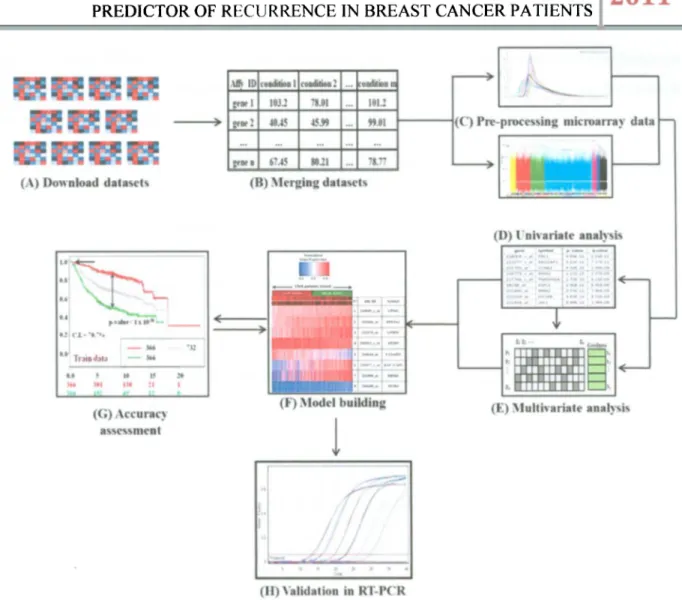
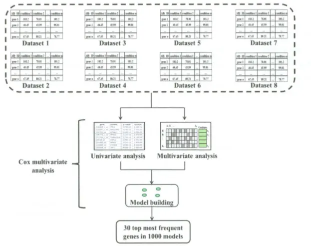
(31) D E V E L O P M E N T OF M U L T I V A R I A T E B I O M A R K E R G E N E S A S A P R O F I L E P R E D I C T O R OF R E C U R R E N C E I N B R E A S T C A N C E R P A T I E N T S. 2011. CHAPTER 3. MATERIALS AND METHODS 3.1 Methodology to develop multivariate biomarker genes A flow-chart o f the present methodology is sketched in Figure 3.1. This methodology consists o f the following steps: 1. Data collection o f available public microarray data with recurrence. clinical. information. 2. Merge every data in one huge dataset. 3. Dataset pre-processing 4. Univariate analysis 5. Multivariate analysis 6. M o d e l building 7. Accuracy assessment 8. Validation in R T - P C R. INSTITUTO TECNOLOGICO Y DE ESTUDIOS SUPERIORES DE MONTERREY. Page 19.

(32) D E V E L O P M E N T OF M U L T I V A R I A T E B I O M A R K E R G E N E S A S A P R O F I L E PREDICTOR OF R E C U R R E N C E IN BREAST C A N C E R PATIENTS. Figure 3.1: Flow-chart of the methodology proposed to develop robust biomarker genes. (A) Nine public microarray data, (B) Data was merged in one huge dataset, (C) Dataset was pre-processed, (D) Univariate analysis, (E) Multivariate analysis to find the best set of biomarker genes. (F) The set of genes was built and assessed to ensure its performance as good predictor of recurrence in breast cancer patients. E) Validation of the biomarker genes by RT-PCR.. For the Affymetrix © Technology has two different sets o f guidelines are commonly used in microarray studies: the Affymetrix © guidelines (Affymetrix, 2002) and the Bioconductor guidelines (Gautier et al. 2004). In the Affymetrix system, the raw image data are stored in so-called D A T files. Currently. Bioconductor software does not handle the image data, and the starting point for most analyses is. INSTITUTO TECNOLOGICO Y DE ESTUDIOS SUPERIORES DE MONTERREY. Page 20.

(33) D E V E L O P M E N T OF M U L T I V A R I A T E B I O M A R K E R GENES A S A PROFILE P R E D I C T O R OF R E C U R R E N C E I N B R E A S T C A N C E R P A T I E N T S. 2011. the C E L files. These are the result o f processing the D A T files using Affymetrix software to produce estimated probe intensity values. Each C E L file contains data on the intensity at each probe on the Gene-Chip, as well as some other quantities. All. microarray. data. was. downloaded. in. CEL. files. from. G E O public. web. site. (http://www.ncbi.nlm.nih.gov/geo/).These microarray datasets have been used with "gpl96" and "gpl570" platforms (platform accession for Affymetrix. H G U 1 3 3 A microarrays and H G -. U133Plus 2.0 respectively), because these two particular arrays have 22,277 probe sets in common. The use o f nearly identical platforms is important since different platforms for geneexpression profiling measure expression o f the same genes with varying precision, on different relative scales, and different dynamic ranges (Tan et al. 2003). Furthermore, we downloaded them based in their content for breast cancer patients more than 50 patients with available recurrence clinical information as show the Table 3.1. Nine studies published such raw data in G E O (GSE1456, GSE2034, GSE2990, GSE4922, GSE6532, GSE7390, GSE9195, GSE12093, and GSE16391) which were downloaded and merged in one called meta-dataset. Table 3.1: Nine datasets downloaded from GEO Database with respectively amount of patients. Authors-GEO. N° patients. References. Desmedt-GSE 16391. 55. Desmedt et al. 2009. Desmedt-GSE7390. 198. Desmedt et al. 2007. Ivshina-GSE4922. 249. Ivshina et al. 2006. Loi-GSE6532. 225. Loi et al. 2007. Loi-GSE9195. 77. Loi et al. 2008. Pawitan-GSE1456. 159. Pawitan et al. 2005. Sotiriou-GSE2990. 189. Sotiriou et al. 2006. Wang-GSE2034. 286. Wang et al. 2005. Zhang-GSE 12093. 136. Zhang et al. 2009. Total. 1574. This meta-dataset contains different clinical marker status as lymph node negative or positive and/or estrogen receptor negative or positive found in each datasets downloaded, as shows in the Table 3.2, moreover most patients did not have treatment before the primary surgery (1477 patients), as shows the Table 3.3, but they also have been treated with different. INSTITUTO TECNOLOGICO Y DE ESTUDIOS SUPERIORES DE MONTERREY. Page 21.

(34) D E V E L O P M E N T OF M U L T I V A R I A T E B I O M A R K E R G E N E S A S A P R O F I L E P R E D I C T O R OF R E C U R R E N C E I N B R E A S T C A N C E R P A T I E N T S. 2011. treatment protocols after the surgery, as shows the Table 3.4. This variety o f profiles make it hard to analyze them, but it is one o f the principal objectives proposed, it is the development o f a methodology to find multivariate biomarker genes for evaluating every breast cancer patients no matter the clinical profile. Table 3.2: Clinical marker status. The table shows two columns of lymph node (LN) and estrogen receptor (ER) status; both columns show the amount of patients that present clinical marker in each dataset downloaded. Lymph node status. Authors-GEO. Estrogen receptor status. LN-. LN+. Desmedt-GSE 16391. 22. 33. Desmedt-GSE7390. 198. 64. 134. Ivshina-GSE4922. 159. 81. 9. 34. 211. 4. Loi-GSE6532. 97. 113. 15. 11. 202. 12. Loi-GSE9195. 41. 36. Pawitan-GSE1456. Unknown. ER-. ER+ 55. 77 159. Sotiriou-GSE2990. 153. Wang-GSE2034. 286. Zhang-GSE12093. 136 1092. Total. 30. Unknown. 159. 6. 34. 149. 77. 209. 6. 136 293. 189. 1173. 220. 1574. 181. 1574. Table 3.3: Clinical treatment information pre-surgery. The therapy pre-surgery column shows 1477 patients without treatment before the surgery and 97 patients received neo adjuvant and tamoxifen therapy. Therapy pre-surgery Authors-GEO None Desmedt-GSE16391 Desmedt-GSE7390 Ivshina-GSE4922 Loi-GSE6532 Loi-GSE9195 Pawitan-GSE1456 Sotiriou-GSE2990 Wang-GSE2034 Zhang-GSE 12093 Total. 35 198 249 225. Neo adjuvant therapy. _ ., Tamoxifen. 20. 77 159 189 286 136 1477. 20. 77. 1574. INSTITUTO TECNOLOGICO Y DE ESTUDIOS SUPERIORES DE MONTERREY. Page 22.

(35) D E V E L O P M E N T OF M U L T I V A R I A T E B I O M A R K E R GENES A S A PROFILE PREDICTOR OF R E C U R R E N C E IN B R E A S T C A N C E R PATIENTS. 2011. Table 3.4: Clinical treatment information post-surgery. The post-surgery column shows different amounts of patients treated for each treatment protocols used according with each dataset downloaded. Therapy post-surgery Authors-GEO None Desmedt-GSE 16391 Desmedt-GSE7390 Ivshina-GSE4922 Loi-GSE6532 Loi-GSE9195 Pawitan-GSE1456 Sotiriou-GSE2990 Wang-GSE2034 Zhang-GSE12093 Total. 3.1.2. Endocrine therapy. Tamoxifen. Radiotherapy. Systemic therapy. Unknown. 55 198 142. 66 12. 41. 214 77 159 64. 12. 121. 136 490. 125 286 751. 159. 41. 1574. Pre-processing microarray data These C E L files are processed to get measures (intensities) o f each probe per sample. using different methods. Measurements on microarrays may be systematically biased by diverse effects such as efficiency o f R N A extraction, reverse transcription, label incorporation, exposure, scanning, spot detection, etc. Furthermore, there are systematic effects due to characteristics o f the array, such as effects o f different probes (i.e. c D N A or oligos), spotting effects, region effects, pin effects, etc. Therefore, we have to remove systematic noise originating from these varieties o f sources (Quackenbush, 2002). The procedure used to get the expression measures o f each probe can be divided in two steps: Background correction and normalization. Background Correction, this process makes a correction o f background noise. The background is a measurement o f signal intensity caused by auto-fluorescence o f the microarray surface and cross-hybridization. The background correction is a method which does some or all o f the following:. INSTITUTO TECNOLOGICO Y DE ESTUDIOS SUPERIORES DE MONTERREY. Page 23.

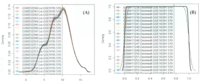
(36) D E V E L O P M E N T OF M U L T I V A R I A T E B I O M A R K E R G E N E S A S A P R O F I L E P R E D I C T O R OF R E C U R R E N C E IN B R E A S T C A N C E R P A T I E N T S •. Corrects for background noise, biological sample preparation.. •. Adjusts for cross-hybridization.. •. Adjusts estimated expression values to fall on proper scale.. MAS 5.0 Background method is outlined in the Statistical Algorithms Description Document (Affymetrix, 2002) and used in the M A S 5.0 software. The chip is divided into a grid o f k (default k = 16) rectangular regions. For each region, the lowest 2% o f probe intensities are used to compute a background value for that grid. Then each probe intensity is adjusted based upon a weighted average o f each o f the background values. The weights are dependent on the distance between the probe and the centroid of the grid. A s shows the Figure 3.2.. Figure 3.2: MAS 5.0 Background correction. This removes the unspecific background intensities of the scanner images (Affymetrix, 2002).. Normalization, it is the process to correct for these systematic errors without removing or altering biological variation. There are two different types o f normalization. These are: within slide normalization and between normalization applied to the. slide normalization. Within normalization. same slide and. refers. to. it is applicable, commonly, for two-dye. technologies correcting for dye and spatial bias. Between normalization is used when at least two slides are analyzed and it requires that both slides are measured on the same scale and that. their. values. measurements.. are. independent. o f the device. parameters. used. to. generate. such. Several methods have been reported and compared for normalization (Park. etal.2003).. INSTITUTO TECNOLOGICO Y DE ESTUDIOS SUPERIORES DE MONTERREY. Page 24.

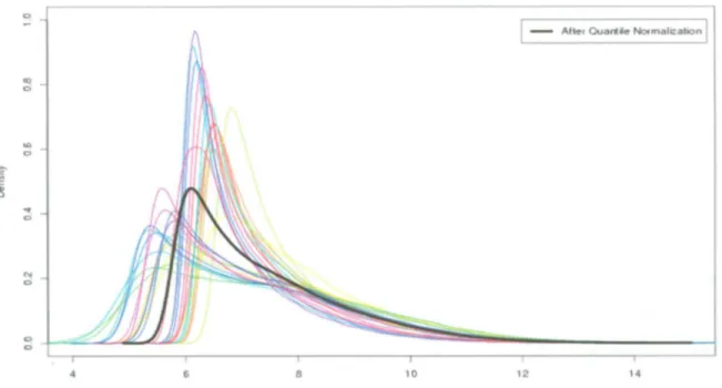
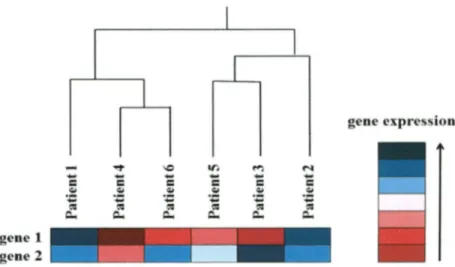
(37) D E V E L O P M E N T OF M U L T I V A R I A T E B I O M A R K E R G E N E S A S A P R O F I L E P R E D I C T O R OF R E C U R R E N C E IN B R E A S T C A N C E R P A T I E N T S Quantile normalization method imposes the same empirical distribution o f intensities to each array. This algorithm forces the distribution o f probe intensities to be the same for all microarrays in the experiment, as shown in Figure 3.3. First an average distribution is calculated and afterwards the distribution o f each microarray is adjusted to have a distribution identical to the pre-calculated average distribution (Bolstad et al. 2003). A downside o f this approach is that a certain probeset will sometimes have exactly the same value across all microarrays.. Figure 3.3: After quantile normalization, the graph shows the black line as result of quantile normalization, modified from Bolstad et al. 2003. Visualization of microarray data, gene expression data is extremely important for biological knowledge discovery. Therefore, it is essential visualization tools for information extracted. Here, this section describes two different visualization tools and parameters used in gene expression analysis.. Hierarchical Clustering is one o f the most common clustering methods. (Eisen et al., 1998) introduced this method to analyze microarray data by organizing genes in a hierarchical tree structure (dendrogram), based on their degree o f similarity. The basic idea is to assemble a set o f items into a binary tree, where items are joined by very short branches i f they are very similar to. INSTITUTO TECNOLOGICO Y DE ESTUDIOS SUPERIORES DE MONTERREY. Page 25.

(38) D E V E L O P M E N T OF M U L T I V A R I A T E B I O M A R K E R GENES AS A PROFILE P R E D I C T O R OF R E C U R R E N C E IN B R E A S T C A N C E R P A T I E N T S each other, and by increasingly longer branches as their similarity decreases. Figure 3.4 illustrates a dendrogram as example.. Figure 3.4: Example of hierarchical representation (dendrogram) produced by a hierarchical clustering analysis of 7 patients.. Heatmap is a graphical representation o f data, where the values o f the variables are represented as colors in a two-dimensional map. This makes possible to visualize a large quantity o f values, such as in microarray data. Although the heatmap is not part o f the clustering algorithm itself, it represents an important step towards visualizing the results. The Figure 3.5 as example illustrates the use o f a heatmap to visualize the gene expressions.. Figure 3.5: Illustrates the use of a heatmap in combination with hierarchical clustering in order to visualize the gene expression. INSTITUTO TECNOLOGICO Y DE ESTUDIOS SUPERIORES DE MONTERREY. Page 26.

(39) D E V E L O P M E N T OF M U L T I V A R I A T E B I O M A R K E R G E N E S A S A P R O F I L E P R E D I C T O R OF R E C U R R E N C E IN B R E A S T C A N C E R P A T I E N T S. It was made using Biom@tec software (http://bioinformatica.mty.itesm.mx:8080/Biomatec/).. The C o x univariate was used to calculate the hazard function model, as shows the Figure 3.7, it has two sections, the first part is the baseline hazard function based in time o f recurrence from patients tested, and the second part is the risk score calculated using the parameter estimation by log likelihood, where this parameter allows to get the beta coefficients used to generate a score, based in this score was calculated the p-values for each gene. Variable ranking was made sorting by lowest p-values, as shows the Figure 3.8. These p-values represent how much the variable is significantly influenced for probability o f recurrence. It does not evaluate the interaction o f each gene.. Figure 3.7: Schematic representation of Hazard function used as Cox univariate model INSTITUTO TECN0L0G1C0 Y DE ESTUDIOS SUPER10RES DE MONTERREY. Page 27.

(40) D E V E L O P M E N T OF M U L T I V A R I A T E B I O M A R K E R GENES AS A PROFILE P R E D I C T O R OF R E C U R R E N C E IN B R E A S T C A N C E R P A T I E N T S. Figure 3.8: It illustrates the beginning of univariate analysis by Cox regression model per gene, after partial log likelihood to finally get a score, and then these genes can be sorted by lowest pvalues.. For typical gene expression microarray data, the huge amounts o f variables that pass the quality control assessment are thousands.. It reveals the exhaustive search for the best. multivariate biomarker consisting o f a few, these multivariate biomarker genes would require inordinate amount of time to figure out who they are. However the present multivariate analysis by P S O modified (Martinez et al. 2010) from Biom@tec software is important multivariate tool to find set o f genes rapidly with high accuracy, where the aim o f this algorithm is generate sets o f genes (models) that contain a specific amount of genes, this algorithm also is able to evaluate the interaction o f each gene to build the model. The methodology began by dividing the meta-data into 50% for training and 50 % for test data. The training data was used to perform the multivariate analysis where the algorithm learn to search the best combination o f genes to generate one model, this process is an evolutionary algorithm based on simulation o f social behavior such as bird flocking, it starts in epoch 1 by creating a population o f particles in random positions. The goodness function based on residuals INSTITUTO TECNOLOGICO Y DE ESTUDIOS SUPERIORES DE MONTERREY. Page 28.

(41) D E V E L O P M E N T OF M U L T I V A R I A T E B I O M A R K E R G E N E S A S A P R O F I L E P R E D I C T O R OF R E C U R R E N C E IN B R E A S T C A N C E R P A T I E N T S found from C o x model, it is then used to evaluate each particle position, the best particle position and best local particle are then found to calculate a new position on the swarm based on last two approaches, after this new position is evaluate by goodness and starts a second epoch, this process repeats 200 times to build one best particle, now called model (Martinez et al. 2010), as shows the Figure 3.9.. Figure 3.9: Schematic representation of Particle Swarm Optimization (PSO). Features (genes = g) are represented in columns whereas particles (p) are represented in rows. Filled cells represents active features whereas inactive features are shown unfilled. The algorithm find the best global and local position based in goodness evaluation to find the best position between both, this process are repeated 200 epoch. Finally, the algorithm finds the best particle or model.. However the generated models from PSO multivariate must be assessed to verify its competence recurrence prediction o f high and low risk in breast cancer patients. Finally, the best model found or built must be validated by comparison o f abilities o f recurrence between training and test data.. INSTITUTO TECNOLOGICO Y DE ESTUDIOS SUPERIORES DE MONTERREY. Page 29.

(42) D E V E L O P M E N T OF M U L T I V A R I A T E B I O M A R K E R G E N E S A S A P R O F I L E P R E D I C T O R OF R E C U R R E N C E IN B R E A S T C A N C E R P A T I E N T S. Once a survival model is built from multivariate analysis, it is time to compare and assess its accuracy. Prognostic Index (PI) is a parameter to compare models (Bovelstad et al. 2007), this approach serves to predict risk of the patients for each model, using: PI = $X. (3.1). where " X " is gene expression value o f each gene into the model and, p" is the coefficient found from log partial likelihood in Cox regression model. The resulted values are then ranked to generate high and low risk groups depending upon the Pit. 7riey w i l l be either larger or smaller according with their median. This approach makes a risk score of each patient.. Figure 3.10: This illustrates the performed risk score in all patients of meta-dataset; it can be then divided in low and high risk groups.. It is a crucial step in the fitting o f the final multivariate model. Thus the methodology use multivariate and univariate approaches to make models with high accuracy. It will be called C o x multivariate analysis.. Concordance Index (CI) is one o f the most commonly used performance measures o f survival models. It can be interpreted as the fraction o f all pairs o f subjects whose predicted survival times are correctly ordered among all subjects that can actually be ordered. In other words, it is the probability o f concordance between the predicted and the observed survival, (Haibe-Kains, et al. 2008). The CI is expressed as INSTITUTO TECNOLOGICO Y DE ESTUDIOS SUPERIORES DE MONTERREY. Page 30.

(43) D E V E L O P M E N T OF M U L T I V A R I A T E B I O M A R K E R G E N E S A S A P R O F I L E PREDICTOR OF R E C U R R E N C E I N B R E A S T C A N C E R PATIENTS. 2011. (3.2). where r, and rj represent the risk predictors given by the corresponding PI for patients / and j respectively and Q represent all patients pairs (/, j) that meet the criteria that t,<tj and patient / is not censored.. Kaplan-Meier (KM), it estimates the survival function from the survival data, (Kaplan and Meier, 1958). It can be used to measure the recurrence probability for a certain amount o f time after the beginning o f follow-up. The value o f the survival function between successive distinct sampled observations is assumed to be constant. For simplicity, explanations are restricted to the case, where the event o f interest is recurrence. Let S(t) be the probability that an individual from a given population w i l l have a lifetime exceeding t. For a sample from this population o f size N let the observed times until recurrence of N sample members be tl < t2 < t3 ... < tN. (3.3). Let T be the random variable that measures the time o f recurrence and let F(t) be its cumulative distribution function. Then the survival function is given by: S(t) = P[T > t] = 1 - P[T < t] = 1 - F(t). (3.4). The Kaplan-Meier estimator is the nonparametric maximum likelihood estimate o f the survival function S (t). It's of the form. (3-5). where n< is the number "at risk" just prior to time tj, and d, is the number o f recurrence at time t,. With censoring, n* is the number o f patients without recurrence less the number o f losses. It is only those surviving cases that are still being observed that are "at risk" o f an (observed) recurrence.. INSTITUTO TECNOLOGICO Y DE ESTUDIOS SUPERIORES DE MONTERREY. Page 31.

(44) D E V E L O P M E N T OF M U L T I V A R I A T E B I O M A R K E R GENES AS A PROFILE PREDICTOR OF R E C U R R E N C E IN B R E A S T C A N C E R PATIENTS Finally, to summarize the statistical phase to find multivariate biomarker genes began dividing the data in two equal parts for training and test data. The training data was used to learn and generate the models by multivariate analysis, after the built model should be assessed by concordance index, and finally the model should be compared its accuracy using training and test data, as shows the Figure 3.9.. Figure 3.11: Schematic representation of statistical phase to find multivariate biomarker genes, the meta-data was divided in two equal parts, the training data is used to make the multivariate algorithm based in PSO, this algorithm build model to be assessed by concordance index, and the built model is compared and validated with training and test data using Kaplan Meier methods to visualize the behavior of this model.. INSTITUTO TECNOLOGICO Y DE ESTUDIOS SUPERIORES DE MONTERREY. Page 32.

(45) D E V E L O P M E N T OF M U L T I V A R I A T E B I O M A R K E R GENES A S A PROFILE P R E D I C T O R OF R E C U R R E N C E I N B R E A S T C A N C E R P A T I E N T S. 2011. 3.2 Validation by real time PCR To validate multivariate biomarker genes found, the quantification o f the expression level o f each gene between different samples by real time P C R is necessary to find out if the model is able to predict recurrence in breast cancer patients. This process is the relative quantitation o f gene expression. For this validation was required the clinical information o f patients, real time P C R experiments and data analysis. 3.2.1 Clinical Information of patients Primary breast cancer tumors were obtained from 10 women treated at Centro de Diagnostico y Tratamiento Integral de mama o f San Jose Tec de Monterrey Hospital from 2007 to 2009. The clinical information collected were age o f patients, months o f followed up, treatment received and presence or absence o f recurrence during the time followed up. The average age o f patients was 49.9 (median 45; range 39-72) and median followed-up was 25 months (range 18-29). A l l patients have not had recurrence during their followed-up and they have different medical treatments currently. The clinical items are shown in detail in Table 3.5. Samples were taken for experimental analysis after receiving patient's consent. Tissue samples were stored at-80°C in buffer RNAlater (Ambion). R N A was extracted using RiboPure™ K i t (Ambion), the R N A concentration o f each sample was measured using Gene Quant Pro Spectrophotometer (Amersham Biosciences), and the average o f R N A concentration was 224ng/ul (range 28-588), as shows Table 3.5.. INSTITUTO TECNOLOGICO Y DE ESTUDIOS SUPERIORES DE MONTERREY. Page 33.

(46) D E V E L O P M E N T OF M U L T I V A R I A T E B I O M A R K E R G E N E S A S A P R O F I L E PREDICTOR OF R E C U R R E N C E IN B R E A S T C A N C E R PATIENTS. 2011. Table 3.5: Clinical information of patients, this illustrates in detail each clinical item of patients; in addition, it shows the variety of protocol treatments of patients, and their RNA concentrations. N° 1 2 3 4 5 6 7 8 9 10. Sample ID M52 M56 M63 M79 M80 M82 M85 M87 M89 M90. Age 43 48 63 42 46 39 72 44 62 40. Follow-up (months). Treatment. Recurrence. 23 24 28 25 25 26 20 18 28 29. Tamoxifen Hormonal therapy Docexatel Taxool + Herceptin Hormonal therapy Quimiotherapy Tamoxifen Quimiotherapy Tamoxifen Quimiotherapy. No No No No No No No No No No. Recurrence (Event = "1", Censored = "0") 0 0 0 0 0 0 0 0 0 0. RNA Concentration (ng/ul) 84 545 489 111 28 588 98 180 268 527. 3.2.2 Validation of the multivariate biomarker genes by real time P C R Real-time Polymerase Chain Reaction ( R T - P C R ) has the ability to monitor the progress of the P C R as it occurs. Data is therefore collected throughout the P C R process, rather than at the end o f the P C R . In real-time P C R , reactions are characterized by the point in time during cycling when amplification o f a target is first detected rather than the amount of target accumulated after a fixed number o f cycles. The higher the starting copy number o f the nucleic acid target, the sooner a significant increase in fluorescence is observed. Real-time P C R begins with the reverse transcription o f R N A into c D N A , and is followed by P C R amplification o f the c D N A . R N A is transcribed into single-stranded c D N A using random primers, gene-specific primers, or oligo-dT primers that specifically hybridize to the poly-A tail o f m R N A s . The quantity o f c D N A is determined during the exponential phase o f P C R by the detection o f fluorescence signals that exceed a certain threshold (Wong and Medrano, 2005). Fluorescence signals are generated by fluorophores such as Sybr Green dye incorporated into the P C R product (used in current thesis)or by fluorophores which are coupled to short oligonucleotide probes. In real-time P C R , the level o f R N A transcripts is calculated from. INSTITUTO TECNOLOGICO Y DE ESTUDIOS SUPERIORES DE MONTERREY. Page 34.

(47) D E V E L O P M E N T OF M U L T I V A R I A T E B I O M A R K E R G E N E S A S A P R O F I L E PREDICTOR OF R E C U R R E N C E IN B R E A S T C A N C E R PATIENTS. 2011. the number o f the P C R cycle at which the threshold is exceeded. This cycle is called the threshold cycle (CT) or the crossing point (Schefe et a/.2006).. Reverse Transcription (RT), the c D N A was made by QuantiTect Reverse Transcription K i t (Qiagen), R T Primer M i x was used to synthesize c D N A for quantitative, real-time two-step R T P C R . The R N A concentration o f each sample was adjusted to get 40 ng/ul after the reverse transcription in a total volume o f 20ul. The procedure used to make c D N A was: 1. Thaw template R N A on ice. Thaw g D N A Wipeout Buffer, Quantiscript. Reverse. Transcriptase, Quantiscript R T Buffer, R T Primer M i x , and RNAse-free water at room temperature (15-25°C). 2.. Prepare the genomic D N A elimination reaction on ice, as shows Table 3.6. Table 3.6: Set up of genomic DNA elimination reaction.. Component. Volume/reaction. Final concentration. g D N A Wipeout Buffer,7x. 2ul. lx. Template R N A. variable. Depend on R N A concentration. RNAse-free water. variable. Total volume. 14ul. 3. Incubate for 2 min at 42°C. Then place immediately on ice. 4. Prepare the reverse-transcription master mix on ice, as shows Table 3.7. Table 3.7: Set up reverse transcription reaction,. Component _ Reverse-transcription master mix. Volume/reaction. Quantiscript Reverse transcriptase. 1 ul. Quantiscript R T buffer, 5x. 4ul. R T primer mix. lul. Final concentration. lx. Template RNA Entire genomic D N A elimination reaction (step 3). 14ul (add at step 5). Total volume. 20ul. INSTITUTO TECNOLOGICO Y DE ESTUDIOS SUPERIORES DE MONTERREY. Page 35.

(48) D E V E L O P M E N T OF M U L T I V A R I A T E B I O M A R K E R G E N E S A S A P R O F I L E P R E D I C T O R OF R E C U R R E N C E I N B R E A S T C A N C E R P A T I E N T S. 2011. 5. A d d template R N A from step 3 (14 jal) to each tube containing reverse-transcription master mix. 6. Incubate for 22 min at 42°C. 7. Incubate for 3 min at 95°C to inactivate Quantiscript Reverse Transcriptase. 8. Store at -20C°. For the real time P C R experiments were designed 11 set o f primers (from ten genes + housekeeping gene), as shows Table 3.8, these primers were designed to be exon-spanning to avoid amplification o f genomic D N A , i f the template could be contaminated with it. Detection temperature was determined above unspecific/primer-dimer melting temperature Table 3.8: It illustrates the sequences of 10 set of primers of the multivariate biomarker genes and 1 set of primers of the housekeeping gene.. N°. Symbol Gene. Forward Primer (5'-3'). 1. RACGAP1. AATGCCTTTTCAACACCACA. GTGGAACGGACTCTCTGTGA. 2. RRM2. ACAGAAGCCCGCTGTTTCTA. CCCAGTCTGCCTTCTTCTTG. 3. PPFIA1. TTTTGGTCATGGGGACTGAT. CCACGAATGTCCTTTGGTCT. 4. AATCAGCAAGGGATTGGCAGCA GAAATGGGTGGGACTGAGAA. AAGGGTGGCTCTGACTTTGACT. 5. C12orf35 SF3B3. 6. AP2B1. GCAGTGGGACAATCCTTCAT. AGGAGCCACATATCCACCAG. 7. GPR56. GCAATGTGTGTTCTGGGTTG. GGAGGCTCAGGTAGTGCTTG. 8. VPS41. CGGTCTTGGATGAACAGATG. GGCACATTGGTGATTCTTTG. 9. CFTR/MRP. CAAGCACGAGTCTTCTGACG. AAGATCCACACAACCCTTCG. 10. CCNA2. GCCTTGTCTCATGGACCTTC. CTCTGGTGGGTTGAGGAGAG. 11. GAPDH. AAGGTCGGAGTCAACGGATT. TGAGGTCAATGAAGGGGTCA. Reverse Primer (5'-3'). CCGAGTGCGAGTATCAGACA. Quantitative PCR by Sybr Green Dye was performed using Rotor-Gene™ 3000 (Corbett Research).PCR products were detected using the S Y B R ® Green I. To make the reaction setup was used QuantiTect ® S Y B R ® Green P C R (Qiagen). The procedure was standardized to lOul as total reaction volume; furthermore all reactions were performed for triplicate. The procedure was used: 1. Thaw 2x QuantiTect S Y B R Green P C R Master M i x , template D N A or c D N A , primers, and RNAse-free water. M i x the individual solutions. INSTITUTO TECNOLOGICO Y DE ESTUDIOS SUPERIORES DE MONTERREY. Page 36.

(49) D E V E L O P M E N T OF M U L T I V A R I A T E B I O M A R K E R GENES A S A PROFILE P R E D I C T O R OF R E C U R R E N C E I N B R E A S T C A N C E R P A T I E N T S. 2011. 2. Prepare a reaction mix, as shows Table 3.9. 3. A d d template c D N A sample (10 ng/reaction) to the individual P C R tubes containing the reaction mix.. Table 3.9: Set up the real time PCR reaction.. Component. Volu me/reaction. Final concentration. 2x QuantiTec S Y B R Green P C R Master Mix. 5ul. lx. Primer A (2.5uM). 0.8ul. 0.2uM. Primer B (2.5uM). 0.8ul. 0.2uM. Template c D N A (40ng/ul). 0.25ul. 10 ng/reaction. RNAse-free water. 3.15ul. Total reaction volume. lOul. 4. Real-time cycler conditions, as shows Table 3.10.. Table 3.10 Real-time cycler conditions.. Step. Time. Temperature. Additional Comments. P C R initial activation. 15min. 95°C. HotStartTaq D N A Polymerase is activated by the heating step. Denaturation. 20s. 94°C. Annealing. 15s. 64°C. Extension. 21s. 72°C. Number o f cycles. 40 cycles. It is the best condition for all primers used in real time P C R experiments. PCR Amplification Efficiency, to make the R T P C R o f the samples the main requirement is get a good P C R amplification efficiency. P C R amplification efficiency is the rate at which a P C R amplicon is generated commonly expressed as a percentage value. If a particular P C R amplicon doubles in quantity during the geometric phase o f its P C R amplification then the P C R assay has 100% efficiency.. INSTITUTO TECNOLOGICO Y DE ESTUDIOS SUPERIORES DE MONTERREY. Page 37.