Modeling of the Division Point of Different Propagation Mechanisms in the Near-Region Within Arched Tunnels

Modeling of the Division Point of Different Propagation

Mechanisms in the Near-Region Within Arched Tunnels

Ke Guan • Zhangdui Zhong • Bo Ai • Cesar Briso-Rodriguez

Abstract An accurate characterization of the near-region propagation of radio waves inside tunnels is of practical importance for the design and planning of advanced communication systems. However, there has been no consensus yet on the propagation mechanism in this region. Some authors claim that the propagation mechanism follows the free space model, others intend to interpret it by the multi-mode waveguide model. This paper clarifies the situation in the near-region of arched tunnels by analytical modeling of the division point between the two propagation mechanisms. The procedure is based on the combination of the propagation theory and the three-dimensional solid geometry. Three groups of measurements are employed to verify the model in different tunnels at different frequencies. Furthermore, simplified models for the division point in five specific application situations are derived to facilitate the use of the model. The results in this paper could help to deepen the insight into the propagation mechanism within tunnel environments.

Keywords Break point • Division point • Modeling • Near-region • Propagation • Tunnel

1 Introduction

Propagation modeling in tunnels has always been a complex task in the design of wire-less communication systems. Among all cross-sectional shapes, arched tunnels are the most typical ones for modern road, railway and subway systems and therefore it is important to investigate the propagation modeling of this type of tunnels. Two most common categories

K. Guan (IHI) • Z. Zhong • B. Ai

State Key Laboratory of Rail Traffic Control and Safety, Beijing Jiaotong University, Beijing 100044, China e-mail: [email protected]

C. Briso-Rodríguez

(a) _(O.R.O)

/

J

r

(-/i.O.Oi1,

a

i

(OAÜ

>tr

b

^

\ \

S «

J

( A 0,0)

(0.-K.0)

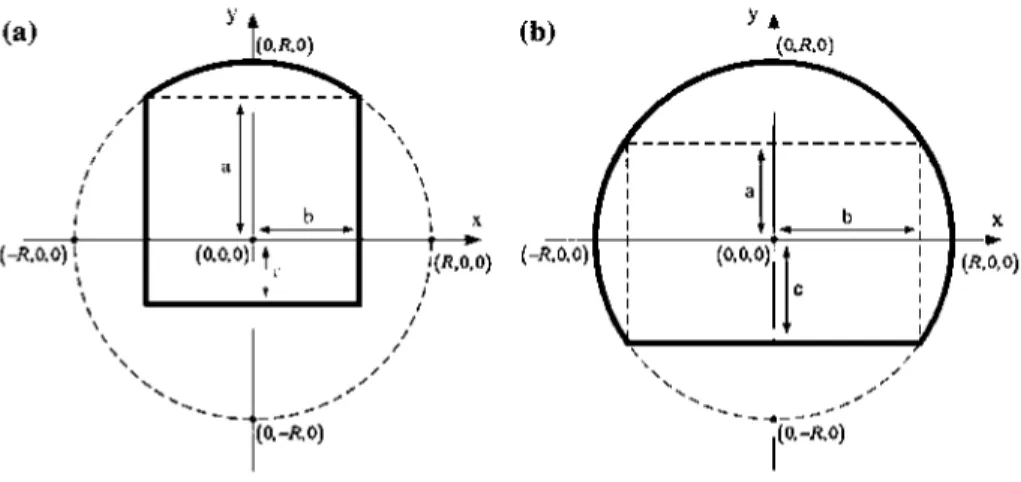
Fig. 1 A cross-section of the arched tunnel "Type I" (a) and "Type II" (b)

(0.-K.0)

of arched tunnels are: Type I,f6 depicted in Fig. la, which consists of flat side walls, flat bottom and arched top, and Type IIf6 shown in Fig. lb, which consists of arched side walls, arched top and flat bottom. We have carried out a wide range of propagation measurement campaigns in both types of arched tunnels, in a real subway tunnel as well as in an operational railway tunnel in Spain.

A number of propagation models inside tunnels presented in the last four decades indicate that there is a "critical distance" [1,2], usually called the break point [1-3]. In front of and behind this break point, the propagation characteristics including path loss, shadow fading and small-scale fading are considerably different [2,4,5]. Hence, the zone in front of the break point is defined as the near-region; correspondingly, the segment behind it is defined as the far region [6],

The distance from the transmitter to the break point is defined as [1]

ZNR

= Max

/W

H

\

where W denotes the width of the rectangular tunnel, H denotes the height of the rectangular tunnel, and X is the signal wavelength in metres, respectively. This equation can be applied in case of arched tunnels, as the electromagnetic field distribution and the attenuation of the modes in arched tunnels are almost the same as in rectangular tunnels [7]. It is worth noting that ZNR is inversely proportional to the wavelength.

the transmitter. Therefore, the propagation mechanism in the near-region becomes a major issue.

The propagation characteristics in the far region inside tunnels follow the fundamental-mode waveguide mechanism [1,2,6]; however, there has been no consensus on the prop-agation in the near region within tunnels. Some dissertations are inclined to interpret the propagation in front of the break point with a single ray (free space) theory [6,16], others contend that it should be described by a multi-mode waveguide model [1,2,17]. All the cited publications treat the near-region as a whole and interpret the propagation situation by a single mechanism. In fact, there has been much evidence that proves that both propagation mechanisms exist simultaneously. The free space mechanism is established at short ranges and the multi-mode propagation mechanism occurs at longer ranges. Thus, interpreting the propagation in the near-region by merely one mechanism and corresponding model limits the prediction accuracy. To overcome this limitation, a novel structure with a clear division point between different propagation mechanisms is highly desired. The authors of [ 18] divide the near-region into two segments and model the path loss in each segment. Concerning their division point, the model in the free space is employed to calculate the location [18]. This result has been proven to be reasonable, but it is valid only under certain conditions [19].

In order to clarify the propagation situation in the near-region of tunnels, it is essential to establish a general model for the accurate location of the division point between different mechanisms.

2 Analytical Modeling of the Propagation Mechanisms and Their Division Point

2.1 Geometrical and Electrical Modeling for the Tunnel

From a theoretical point of view, arched tunnel can be regarded as an equivalent rectangular tunnel. Therefore in this paper, the arched tunnel is treated as an equivalent oversized imper-fect hollow rectangular waveguide. The size of the equivalent rectangular waveguide can be computed by taking the main horizontal dimension W close to the tunnel's floor size and computing the vertical dimension H by using the "rule of thumb", i.e.,

H = J4R2 - W2 (2)

This idealized geometry is common in modern road and railway tunnels [20],

In order to use the geometrical and modal analysis, the following parameters are required: - A coordinate system: a three-dimensional Cartesian coordinate system, with its origin

located at an angle of the equivalent rectangular tunnel.

- Geometrical dimensions: width of the equivalent rectangular tunnel: W, height of the equivalent rectangular tunnel: H. The coordinates of the transmitter, receiver and middle point on the line of sight between transmitter and receiver are Pt (xt, yt, zi), Pr (xr, yr, zr) and PQ (XO, yo, ZO); their relations are expressed by

xr +x, yr + y, zr + Zt ...

xo = - ^ - . y o = - ^ - . z o = —^ (3)

2.2 Propagation Loss Owing to Different Propagation Mechanisms 2.2.1 Propagation Loss in the Free Space Propagation Segment

In the adjacent region of the transmitter antenna, the angles of incidence from the ray to the wall (vertical and horizontal) are high, resulting in high attenuation of reflected rays, whereas the path difference between direct and reflected rays may also cause additional attenuation. Thus, only the direct ray significantly contributes to the strength of the received signal. The channel loss in this segment follows the free space loss attenuation [21]

>2

PL(dB) = - 1 0 log ₁₀ XA {ATT)1 \Zr ~ ZtY

(4)

where \zr — Zt I is the distance between transmitter and receiver in metres, and k is the signal wavelength.

2.2.2 Propagation Loss in the Multi-Mode Waveguide Segment

According to the modal theory, a rectangular tunnel can be regarded as an oversized imper-fect hollow rectangular waveguide. Since the UHF is considerably higher than the cutoff frequency of the fundamental modes, a wide range of Emn multiple modes propagate inside tunnels when the free space segment ends [18]. Using modal theory, the losses of horizontally and vertically polarized Emn modes can be given by

a {m,n)h= 4.343k2 ( ™ll= + , "—=) dB/m (5)

a{m,n)v = 4.343X2( "? = + " * l \ dB/m (6)

With the propagation constants offered above, the propagation loss in the multi-mode wave-guide segment can be calculated by considering the modes for both polarizations

.

J

(dB) = Wlg

¿ = 1 ; = 1

(7)

2.3 Division Point Between Different Propagation Mechanisms 2.3.1 The Core Idea of Localization of the Division Point

In optics and radio communications, Fresnel zones are elliptical in shape with the transmitter and receiver antenna at their foci. The innermost ellipsoid is called the first Fresnel zone, which contains the strongest radio signal.

direct ray and the rays reflecting off those objects out of the first Fresnel zone may cause additional attenuation. All these render the already weak reflected rays even weaker. As a consequence, only the direct ray significantly contributes to the strength of the received signal. Thus, the free space loss channel model can be applied in this region.

Subsequently, with the receiver moving further away, the first Fresnel zone will touch the wall at one point, then the reflection starts to occur inside the first Fresnel zone and effectively reinforces the signal strength at the receiver. This means the end of the free space propagation mechanism.

Further from that point, the first Fresnel zone becomes unclear along with its own expan-sion. The effect can be treated as the process in which the walls of the tunnel penetrate the first Fresnel zone and generate many effective reflected rays, which are regarded as modes in waveguide theory. Hence, the multi-mode waveguide propagation mechanism starts.

Based on the above analysis, it is manifest that the point where the first Fresnel zone is tangent to the walls of the tunnel is the division point between the two propagation mecha-nisms. However, locating it is definitely not an easy task. Since the interaction between the first Fresnel zone and the walls depends on a great number of factors, such as the locations of the transmitting antenna and receiving antenna, the dimensions of the tunnel, the oper-ating frequency, etc., the computational time would be intolerable if all the elements were considered when we track the interaction and its change law. Hence, in order to accelerate the process, it is desirable to find a simple parameter representing the interaction.

According to geometry, it is easy to determine the distance between the tangent line/curve (of the Maximum Fresnel zone plate and the walls) and the middle point (of the line of sight between transmitter and receiver). If this distance is larger than the radius of the Maximum first Fresnel zone plate, the first Fresnel zone can be treated as almost clear. It is true that in this case some parts inside the first Fresnel zone could still be blocked. But since the first Fresnel zone is a flat ellipsoid, such kind of slight obstruction does not lead to many effective reflected rays or obvious diffractive loss. Hence, the free space propagation model can still work. When this distance is smaller than the radius, that means even the widest part of the first Fresnel zone is blocked, more severe obstruction occurs in the other parts. Thus, the relative relation of this distance and the radius can be employed to reflect the interaction between the first Fresnel zone and the walls to some extent. Furthermore, the location of the division point can be deduced when the distance and the radius are equal.

2.3.2 Two Types of Arched Tunnels

To grasp the accurate propagation mechanism situation, it is essential to model the location of the division point between the free space propagation segment and the multi-mode wave-guide segment. Figure la and b demonstrate the cross-sectional geometry for both types of arched tunnels. It is noteworthy that both arched tunnel "Type I" and "Type II" can be seen as a combination of a circular and a rectangular tunnel, but in different configurations. Hence, the division point can be modeled in circular tunnel and rectangular tunnel independently, then determined by their specific combinations.

2.3.3 Geometrical Analysis in the Case of Circular Tunnel

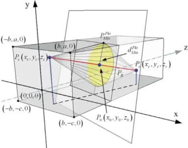
Fig. 2 Detailed schematic diagram of the propagation inside circular tunnels with the first Fresnel zone

clearance

geometry, the surface of the circular tunnel is the set of points, the coordinates of which x, y satisfy the following equation

x2 + y2 = R2 (8)

with z-coordinates completely arbitrary. The Maximum Fresnel zone plate can be expressed by a plane of a general type

(Xr-Xt)(X-^) + (yr-yt)(y-y-^)

+ (Zr-Zt)(z-Z-^)=0 (9)

The intersection between the Maximum Fresnel zone plane and the surface of circular tunnel is a curve which can be defined as

' (xr-xt) (x - *±2.) + (yr - yt) (y - *±*)

+ (Zr ~ Zt) (Z ~ ¡¿¡I.) = 0 (10) x2 + y2 = R2

If we define the first equation as a function / (x, y, z) as

f (x,y,z) = (x

-x

)lx —

\ + {y

-yt)(y —

. J

+ (Zr-Zt)(z-Z-^j (11)

and the second equation as a function g (x, y, z) as

g (x, y, Z) = x2 + y2- R2 (12)

/ Zr + Zt \

+

{

Z

-—)

2

+ S-f(x,y,z) + fi-g(x,y,z) (13)

where f, /x are the Lagrange multipliers. By seeking a partial derivative of x, y and z, respec-tively, Eq. 13 can be transformed as follows:

3 F

— = 2 ( x — ) + f • (xr - xt) + n • 2x = 0 (14)

2

(

l

-*±*)

+ i ( &

( xr + xt\ ( yr + yt\

+ (Zr ~ Zt) l z 0 ) dF

—- = (xr - xt)

0 (17) V z /

— = x2 + y2 - R2 = 0 (18)

d/J,

By seeking the simultaneous solution of (14)—(18), the coordinate of intersection point with the minimal distance to PQ (XQ, yo, zo) can be obtained: p^[n (xClr (zr), yClr (zr), zClr (zr))-Therefore, the minimal distance between Po and the intersection (curve) between the Maxi-mum Fresnel zone plane and the wall of circular tunnel can be expressed as

d-Min (zr)

[ ( x - f e

r

) - ^ )

2 +

( ^ ( z

r

) - ^ )

2

+ ( ^ f e ) - ^ )

2 +

(z-(z

r

)-^)

2

]

2.3.4 Geometrical Analysis in the Case of Rectangular Tunnel

As shown in Fig. 3, the tunnel is treated as a rectangular tunnel. The process is similar to the circular tunnel but easier, since the wall of the rectangular tunnel is not a curved surface but a plane surface, which can be expressed as follows:

Ax + By + Cz + D = 0 (20)

The tangent line is expressed by the simultaneous Eqs. 9 and 20. Similarly, define (9) and (20)

as function f (x, y,z) and g (x, y,z), respectively. Using the Lagrange multiplier method, we construct the objective function as follows:

/ xr + x, \ ( yr + y, \

{

x

-—)

+

v-—)

( Zr+ZtV

\

- — )

G (x, y,z,cp, ip) =

2

(-M.0)

(-í-.-c.O)

Fig. 3 Detailed schematic diagram of the propagation inside rectangular tunnels with the first Fresnel zone

clearance

where x/r is the Lagrange multiplier. B y seeking partial derivative of x, y and z, respectively, Eq. 21 can b e transformed to

dG dx dG

dG ~dz dG d<p

dG dip

( xr+xt\ ( yr + yt \

r ~xt) \x — I + (yr -yt)ly — I + ip • (xr — xt) + xfr • Ax = 0

+ <P • (yr ~ yt) + •f • By = 0

+ <P • (zr ~ Zt) + if • Cz = 0

Ax + By + Cz + D = 0

(22)

(23)

(24)

(25)

(26) By solving (22)-(26), the location of the intersection point with the minimal distance to PQ can be obtained: p^n (xpla (zr), ypla (zr), zpla (zr)) • Then, the minimal distance between Po and the intersection (line) are derived as:

d-Min (Zr)

[ ( x - ( z

r

) - ^ )

2 +

( / - f e

r

) - ^ ) '

2.3.5 Division Point Modeling in Arched Tunnels

After deducing the Algorithm of d^ (zr) and d.^" (zr) from circular and rectangular tun-nels, respectively, we need to determine the minimal distance <¿M¿„ (zr) in the arched tunnel case according to the two types of combinations.

Based on the propagation theory, the radius of the first Fresnel zone is determined by

n = J

^Td~

where d\ denotes the distance between the transmitter and the point of interaction between the line of sight and the first Fresnel zone, ¿2 denotes the distance between the receiver and the point of interaction. When the point of interaction is the middle point PQ, then d\ = dpt p0 = ¿2 = dpQ pr = \dpt pr. At this point, the radius gets the maximum value of the

first Fresnel zone plate

riMax (Zr) = T^J"^dptpr (29)

According to the propagation theory, the free space loss channel model can be applied if the first Fresnel zone is free of any obstacles. Therefore, the division point between two prop-agation mechanisms locates at zr which is the minimal positive real root of the following equation

riMax (Zr) = d-Min (Zr) (30)

This means that the Maximum first Fresnel zone plate first touches the surface of arched tunnels; even the widest part of the first Fresnel zone starts to be blocked from this point onwards.

In Fig. 4 the propagation inside the arched tunnel "Type I" with the first Fresnel zone clearance is shown. In "Type I", two vertical walls and the floor in the rectangular tunnel as well as the arched roof in the circular tunnel can possibly obstruct the first Fresnel zone, thus substituting the roof function to (8) and the wall/floor function to (20):

- Left vertical side wall: x = —b; - Right vertical side wall: x = b; - Bottom/Floor: y = —c;

- Arched top/roof: x2 + y2 = R2, \x\ < b, a < y < R;

dMinR &), dPmñR (zr), d ^L (zr) and d^~F {zr) corresponding to the minimal dis-tance from PQ to the intersection (line/curve) on the arched roof, the right/left wall and the floor can be obtained. By using (30), the division point location of zrC^l~R, ZrM?n~R, Zr^iñ1 and ZrMiñ corresponding to the touching of the Maximum first Fresnel zone and the arched roof, right wall, left wall and floor of arched tunnels, respectively, can be derived as:

ZrmñR = Min [Zr \riMax (zr) = d ^R, Zr G R+ } (31)

Min \zr \riMax {Zr) = d^~R, Zr € R+ } (32)

in \zr \riMax (Zr) = d^~L, Zr G R+ } (33)

in \zr \riMax (Zr) = ¿ M ' T ^ Zr G R+ } (34) Pla-R

rMin

Zrl}?-

= Mi,

Fig. 4 Detailed schematic diagram of the propagation inside the arched tunnel "Type I" with the first Fresnel zone clearance

Then, the division point between the two propagation mechanisms inside the arched tunnel "Type I" is located at

zr'-z - Min (zr'-z Cir-R zr'-z Pla-R zr'-z Pla-L 7 Pla-F\ (35)

Figure 5 illustrates the propagation of the clearance of the first Fresnel zone inside arched tunnel "Type II". In "Type II", only the floor in the rectangular tunnel and the arched roof/wall in the circular tunnel can possibly obstruct the first Fresnel zone, thus substituting the arched roof's functions to (8) and the floor's function to (20):

- Floor: y = —c;

- Arched roof: x2 + y2 = R2, -c < y < R;

dM'[n (zr) and dM®~ (zr) can be derived. By employing (30), the division point loca-tion of ZrMi„ ^^Zruin corresponding to the touching of the Maximum first Fresnel zone and the arched roof/floor and the floor of tunnels, respectively, can be obtained:

ZrmñRIW = Min [Zr \r1Max (zr) = dfir-x, ZreR+} (36)

ZrmñF = MÍn [Zr \riMax (Zr) = d¡^~F, Zr € R+ } (37)

Then, the division point inside the arched tunnel "Type II" is located at

zr'-j... ( Cir-R/W Pla-F\ /TON

zr = Min[zrMin ,zrMin J (38)

3 Division Point Model Validation

Fig. 5 Detailed schematic diagram of the propagation inside the arched tunnel "Type II" with the first Fresnel

zone clearance

the operating frequency involves 400 and 900 MHz. Relevant details and parameters in these measurements are cited as follows:

- The first data set consists of the measurements taken in one of the longest tunnels of the new 450-km high-speed train line connecting Madrid and Lleida in Spain [1]: X = 0.33, R = 6.2, x, = 6, y, = 0,zt = 0, xr = 3, yr = 0, A = 0, B = 1, C =

0, D = 3. By seeking the simultaneous solution of (14)—(18), the coordinate of inter-section point with the minimal distance to PQ (XQ, yo, zd) in the circular tunnel can be obtained: p¡J[n (6.2,0, 17.57). By substituting relevant parameter into (9) and (20),

the minimal positive real root of the simultaneous solutions of (22)-(26) is the coordinate of intersection point with the minimal distance to PQ (XQ, yo, zd) in the rectangular

tun-n e l : PmnF (4 5> -3' 5 4-0 3) - By s o l v i ng (36) and (37), zr^¡~R/W = 34.84, z/J^ =

108.07. Hence, according to (38), the division point locates at zr = 34.84 in this case. - The second data set of received signal strength consists of the measurements performed

in a railway tunnel typical for Europe at 400 MHz. The tunnel is 520 m long and originally engineered for a railway, but the line was closed and it is now being used by pedestrians and cyclists [18]: k = 0.75, R = 2.35, x, = 0, y, = 0, zt = 0, xr = 0, yr = 0, A = 0, B =

1, C = 0, D = 1.5. By jointly solving (14)-(18), we can get: p^R/W (0,2.35, 13.48). By simultaneously solving (25)-(29), we can obtain: pM"~ (0, —1.5, 6.85). By solving

(36) and (37), zr^ [n _ J ? / W = 27, zrmñF = 13.65. Then using (38), the division point is

located at zr = 13.65.

Table 1 Comparison of the

division point results for different types of tunnels between the model and the measurements

Tunnel

Railway tunnel in Spain [1] Pedestrian tunnel in

Europe [18]

Road tunnel Austria-Slovenia [18] Frequency (GHz) 0.9 0.4 0.4 Measured result (m) 35 15 15 Theoretical prediction (m) 34.84 13.65 15.41 Transmitter E -1CK

- Measured data

- Multi-mode waveguide • Free space loss model

Break point

-70

Multi-mode waveguide

Near region

2950 3000 3050 3100 Distance (m)

3150 3200

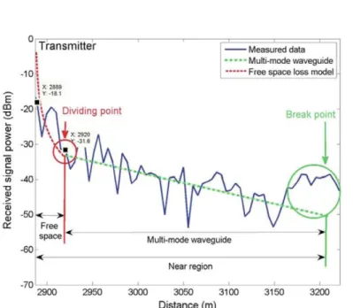
Fig. 6 Comparison between measured and theoretical results on the propagation mechanisms and their

divi-sion points in the near-region within arched tunnels

Table 1 illustrates the comparison of the division point inside tunnels between the model and the measurements. The location of the division point is extracted from the measurements in this way: the free space propagation model was compared with the measured received signal power, then the point, in front of which the fitting is good and behind which is bad, was found. The theoretical location of the division point is predicted by the model pro-posed in this paper. As shown in Table 1, the results from the comparison indicate that the model for the division point is performing well in different types of tunnels at various frequencies.

Fig. 7 a Special situation one; b special situation two; c special situation three; d special situation four; e special situation five

All the validation results and comparison offered above indicate that the analytical model for the propagation mechanisms and their division point in the near-region within arched tunnels presented in this paper is valid and easy to use.

4 Division Point Model Simplification and Discussion

In some applications, the locations of transmitting and receiving antennas, as well as the motion trajectories of mobile stations follow certain rules. In this section, the sim-plified formulas of the diving point model are deduced corresponding to five application situations.

Table 2 Simplification of the division point model in certain special situations

Situation Condition Type Division point zr

yt=yr = Y) Type II Min | - i x '-,

^p-\2 4{R-^/2L

Two (xt = xr = L, Type I Min 4(fl-V2L)

4(b±L)2 4 ( e + £ )2

N2

y, = jV = L) Type II Min -*•—x ¿-, \

Three (xt = xr = 0, Type I Min fe*¿ l í * ± í ¿ , 4 ¿ )

yt =yr = 7) Type II M n ( ± ^ , ± ^ )

Four ( * , = * , = * , Type I Min («£ftt &, Í Í £ + I ¿ )

yt = yr = 0)

Five ( xt= xr= 0 , Type I Min (^, áj¿, á ¿ )

yt = yr = 0) Type II Min ($g-, á ¿ )

By employing the model presented in this paper, the location of the division point can be expressed by simple formulas corresponding to both "Type I" and "Type II", in each special case. Details are shown in Table 2.

All the simplified formulas provide an easy way to determine the location of the areas corresponding to different propagation mechanisms in the near-region, under the realistic application scenarios. Summarizing the general character of the simplified formulas, we have found that the minimal absolute distance between antennas and any of the tunnel sur-faces is the dominant factor in the calculation of these cases. This conclusion can be very useful for the system designer to control different mechanism-based propagation areas in the near-region within tunnels.

5 Conclusion

tunnel. Three groups of measurements have proved that the model is valid in different types of tunnels at different operating frequencies.

Simplified formulas allow the model to be easily applied in many realistic situations. It has been found that in these cases the minimal absolute distance between the antennas and any of the tunnel surfaces dominates the determination of the location of the division point. This conclusion can effectively help system designers to control different mechanism-based propagation areas.

The analysis, approach, and model in this paper can be essential for deeper understanding of the propagation mechanism inside tunnels, and can be used in the realistic radio system design for link and system level simulations.

Acknowledgments We would like to thank the following for their support: the NNSF of China under Grant

60830001, Program for New Century Excellent Talents in University under Grant NCET-09-0206, Beijing NSF 4112048, the Key Project of State Key Lab. of Rail Traffic Control and Safety under Grant RCS2008ZZ006, the Fundamental Research Funds for the Central Universities under Grant 2010JBZ008, and the State Key Lab. of Rail Traffic Control and Safety (Contract No. RCS2010K008), Beijing Jiaotong University.

References

1. Briso-Rodriguez, C , Cruz, J. M., & Alonso, J. I. (2007). Measurements and modeling of distributed antenna systems in railway tunnels. IEEE Transactions on Vehicular Technology, 56(5, Part 2), 2870-2879.

2. Zhang, Y. P., & Hwang, Y. (1997). Enhancement of rectangular tunnel waveguide model. Microwave

Conference Proceedings 1997. APMC '97, 1997 Asia-Pacific, 1, 197-200.

3. Zhang, Y. P., & Hwang, Y. (1998). Characterization of uhf radio propagation channels in tun-nel environments for microcellular and personal communications. IEEE Transactions on Vehicular

Technology, 47, 283-296.

4. Alonso, J., Izquierdo, B., & Romeu, J. (2009). Break point analysis and modelling in subway tunnels. In 3rd European conference on ant. and propag (Vol. 49, pp. 3524-3258).

5. Guan, K., Zhong, Z. H. D., Ai, B., & Briso-Rodriguez, C. (2010). Research of propagation characteristics of break point: Near zone and far zone under operational subway condition. In International confer-ence on communications and mobile computing, communications and information theory symposium (pp. 114-118).

6. Zhang, Y P. (2003). Novel model for propagation loss prediction in tunnels. IEEE Transactions on

Vehicular Technology, 52, 1308-1314.

7. Molina-Garcia-Pardo, J. M., Lienard, M., Nasr, A., & Degauque, P. (2008). On the possibility of interpreting field variations and polarization in arched tunnels using a model for propagation in rectangular or circular tunnels. IEEE Transactions on Antenna Propagation, 56(9), 1206-1211. 8. ETSI ETR 300-3 ed. 1 (2000-02): (2000). Terrestrial Trunked Radio (TETRA); Voice Plus Data

(V+D); Designers' Guide; Part 3: Direct Mode Operation (DMO). 9. [Online]. Available: http://www.uic.asso.fr

10. IEEE Standard for Communications-Based Train Control (CBTC). (1999). Performance and functional requirements, 30.

11. Notice of proposed rulemaking and order FCC 03-324, Federal Communications Commission. Febrary (2003).

12. Mouly, M., & Pautet, M.B. (1992). The GSM system for mobile communications, Paliseau, France. 13. The wireless dictionary Gilb, J.P.K. IEEE standards wireless series (2005).

14. IEEE draft standard for information technology—Telecommunications and information exchange between systems—Local and Metropolitan networks—specific requirements—Part II: Wireless LAN Medium Access Control (MAC) and Physical Layer (PHY) specifications: IEEE 802.11 Wireless Network Management Amendment, March (2010).

15. IEEE standard for local and metropolitan area networks Part 16: Air interface for broadband wireless access systems amendment 1: Multiple relay specification (pp. cl-290) (2009).

17. Klemenschits, T., & Bonek, E. (1994). Radio coverage of road tunnels at 900 and 1800 MHz by discrete antennas. In 5th IEEE international symposium on PIMRC (Vol. 2, pp. 411—415) 18. Hrovat, A., Kandus, G., & Javornik, T. (2010). Four-slope channel model for path loss prediction in

tunnels at 400 MHz. IET Microwaves Antennas and Propagation, 4, 571-582.

19. Guan, K., Zhong, Z. D., Ai, B., & Briso-Rodriguez, C. (2001). Propagation mechanism analysis before the break point inside tunnels. Accepted by IEEE 74th vehicular technology conference. 20. Mariage, P., Lienard, M., & Degauque, P. (1994). Theoretical and experimental approach of the

propagation of high frequency waves in road tunnels. IEEE Transactions on Antennas

Propaga-tion, 42, 75-81.

21. Saunders, S. (2005). Antennas and propagation for wireless communication systems. Chichester, England: Wiley.

Author Biographies

Ke Guan was born in Si Chuan, China, in 1983. He received the

bach-elor degree from Beijing Jiaotong University in 2006. From March, 2009 to August, 2009, he conducted research in Universidad Politéc-nica de Madrid, Madrid, Spain, as a visiting scientist. Since 2010, he is a Ph.D. candidate in the State Key Lab of Rail Traffic Control and Safety at Beijing Jiaotong University. His primary interest is in prop-agation and wireless channel measurements and modeling, especially under high speed condition.

Zhangdui Zhong was born in May 1962. He is now the professor and

Bo Ai was born in Shaanxi Province in China in 1974. He received a B.Sc. Degree from Engineering College of Armed Police Force in 1997, a Master and Dr. degree from Xidian University in 2002 and 2004 in China, respectively. From 2005 to 2007, he worked as a Post Dr. research fellow in Dept. of E & E, state key lab. on microwave and digital communications in Tsinghua University in China and graduated with great honors of Excellent Postdoctoral Research Fellow in Tsing-hua University. He is now working in Beijing Jiaotong University as an associate professor. He is an editorial committee member of journal of "Wireless Personal Communications", "Recent Patents on Electri-cal Engineerin", "Computer Simulations", "Information and Electronic Engineering", an IEEE member and a senior member of Electronics Institute of China (CIE). He has published four books and 73 scien-tific papers in his research area till now. His bio. has been included in Marquis Who's Who in Science and Engineering and Cambridge IBC books. His current interests are the research and applications of OFDM synchronization, HPA linearization techniques and GSM Railway systems.

Cesar Briso-Rodriguez was born in Valladolid, Spain, in 1968. He