Methods for noise reduction in far-field patterns obtained from cylindrical near-field antenna measurements

Methods for Noise Reduction in Far-Field Patterns

Obtained From Cylindrical Near-Field

Antenna Measurements

F. J. Cano-Fácila and M. Sierra-Castañer

Abstract—Two different methods to reduce the noise power in

the far-field pattern of an antenna as measured in cylindrical near-field (CNF) are proposed. Both methods are based on the same principle: the data recorded in the CNF measurement, assumed to be corrupted by white Gaussian and space-stationary noise, are transformed into a new domain where it is possible to filter out a portion of noise. Those filtered data are then used to calculate a far-field pattern with less noise power than that one obtained from the measured data without applying any filtering. Statistical analyses are carried out to deduce the expressions of the signal-to-noise ratio improvement achieved with each method. Although the idea of the two alternatives is the same, there are important dif-ferences between them. The first one applies a modal filtering, re-quires an oversampling and improves the far-field pattern in all directions. The second method employs a spatial filtering on the antenna plane, does not require oversampling and the far-field pat-tern is only improved in the forward hemisphere. Several examples are presented using both simulated and measured near-field data to verify the effectiveness of the methods.

Index Terms—Additive white Gaussian noise (AWGN), antenna

measurements, filtering, modal analysis, noise cancellation, recon-struction algorithms, signal-to-noise ratio.

I. INTRODUCTION

I

N many cases, antenna radiation patterns and other far-field parameters such as gain, directivity, sidelobe level, beam width, etc., cannot be determined directly from measure-ments taken in a field range because the distance to the far-field region may be too long. However, it is well known that those parameters can be obtained using analytical transforma-tions from near-field measurements [l]-[3]. In these cases, the radiation pattern is obtained by processing the near-field data. Therefore, an uncertainly analysis is required to assess the ef-fect of near-field errors on the accuracy of the far-field pattern. References [4]-[6] are examples of studies that examine the re-lationships between the measurement errors and their effects on the far-field using mathematical analyses, simulations, or mea-surement tests.

This paper focuses on random near-field errors, which are always present and are commonly introduced by the receiver

additive noise. In many cases, these errors are negligible in the overall measurement uncertainty thanks to the use of modern receivers and sufficient amplification in the system. However, when measuring ultra-low sidelobe or high-performance an-tennas, noise may significantly alter the radiation pattern and it has to be taken into account in the near-field error budget. Some comprehensive studies for random noise in near-field measurements have already been presented. For the planar system, two independent analyses with similar results have been described in [7], [8]. Both of them start with random errors in planar near-field (PNF) and obtain expressions that represent the signal-to-noise ratio in far-field as a function of the noise power in near-field. A similar study for cylindrical near-field (CNF) measurements was carried out in [9], [10].

The objective of this paper is not to analyze the effect of random near-field errors in the far-field results, but to describe methods to improve the signal-to-noise ratio in the far-field pat-tern by reducing the noise power. This reduction is achieved by representing the acquired near-field data in a convenient do-main where it is possible to filter out a portion of noise. This idea of reducing the noise by means of a filtering in an aux-iliary domain was proposed in [11] and [12] for the spherical near-field (SNF) case. The same idea was used in [13] to im-prove the signal-to-noise ratio in the far-field pattern of an an-tenna as measured in PNF. In this last case, however, a spa-tial filtering on the antenna under test (AUT) plane is employed instead of a modal filtering. In the present work, two different methods to reduce the noise power when measuring an antenna in CNF are proposed. Moreover, a detailed statistical analysis is performed in each case in order to determine the signal-to-noise ratio improvement.

This paper is organized as follows. Section II describes a modal filtering method. In this section, a statistical analysis to determine the signal-to-noise ratio improvement achieved with this first filtering method as well as a study to obtain the relation-ship between that improvement and the required oversampling are carried out. In Section III, the second method based on a fil-tering on the AUT plane is presented. As in the previous section, the statistical properties of the noise in this new domain are de-termined in order to derive the expression for the signal-to-noise ratio improvement. Several results are shown in Section IV by using both simulated and measured near-field data. Conclusions are drawn in Section V.

II. M O D A L FILTERING M E T H O D

Be-cause all the measured data are always noise corrupted, filtering cannot be applied to this initial information and an auxiliary data representation that allows a noise filtering without cancelling out desired information is needed.

As it is well-known, the initial step to determine the far-field pattern from CNF measurements is to calculate two sets of cylindrical modal coefficients (CMCs) [14].

As deduced from [15], the CMC are band-limited in the n—kz

domain, being negligible outside of the visible region defined by

n2 + {kza0)2 < (fco«o)2 (1)

where ao is the radius of the smallest sphere enclosing the AUT. According to (1), in order to avoid the aliasing error when cal-culating the CMC, the maximum admissible sampling spacing in <j) and z is

2fc0 <

2fcoao <

27r

— => Az

Az 27r

A " 21

max A

max 2 a0

(2)

However, the validity region of the far-field pattern obtained from a CNF measurement is limited in elevation. Therefore, a sampling spacing in z larger than a half wavelength is typically used.

If the separation between samples is smaller than the values indicated in (2), more CMC are obtained in the evanescent re-gion, where theoretically have to be negligible. However, due to the presence of undesired contributions, like reflections, diffrac-tions, leakage signals, etc., the calculated CMC may be nonzero outside of the visible region. Therefore, one alternative to cancel the unwanted effects of these contributions is to apply a modal filtering, setting all CMC in the evanescent region to zero. This idea of applying a modal filtering to suppress unwanted con-tributions and, in particular, reflections from the environment, was initially proposed for the CNF case in [16]. This last work was the extension of previous publications whose aim was the reflection suppression in the spherical case [17], [18] and most recently it has been applied in PNF [19] and far-field [20] mea-surements. A general strategy, which also exploits the band-lim-itation properties of the radiated field, to reduce the effect of the clutter noise, valid for arbitrary scanning and source geometries, was proposed in [21 ]. The first noise reduction method proposed in this paper is based on the principle presented in [ 16]. An over-sampling is applied in order to obtain more CMC than required. After that, the evanescent modes are filtered out, removing the noise contribution in this region. Finally, the filtered CMC are used to calculate a far-field pattern with less noise power.

Once the main idea of this method has been described, a sta-tistical analysis to determine the signal-to-noise ratio improve-ment is carried out. In the analysis, a complex white Gaussian and space-stationary noise is considered. Its mean and variance are assumed to be zero and er2f, respectively. Because

expres-sions to calculate the modal coefficients [14] are linear, an inde-pendent analysis can be performed for the AUT contribution and noise. As mentioned before, the CMC associated to the AUT contribution are theoretically zero outside of the region defined by (1). The noise contribution to the CMC can be determined by

considering only the measured near-field white Gaussian noise in <f) and z. Thus, the autocorrelation of the noise in each set of CMC is

flaAWGN(fe^(a,/3)

= E

A(f>2Az2

AWGN*

(*.)

( 4 T T2)2

N* N. dH. (2)

dr («r)

* E E {^EWE^uz^EWE^^z^

U-K2)2 " '—^ ^ ( « r )

(3)

n6A W G N (f e i) ( a , ^ )

= E lAWGN un+a

(k

z

+P)b™

G

"'(k

z

)]

klAtfAz

2

( 2 ) ,

(4TT2)2 HZ>{Ka)

k2Acj>2Az2N4lNzolt

K* ¡=1 t = l

(4TT2)2 H{2){Ka)

6(a,P) (4)

where A(j> and Az are the azimuthal and vertical sampling spacing, respectively, ¿f„ ' is the Hankel function of second kind of order n, &o represents the free-space wavenumber, a is the radius of the measurement cylinder, N$ and Nz stand for

the number of samples along <p and z coordinates, respectively, and K = y/k2, — fcf. The previous expressions are valid when

using an ideal probe. In the case of arbitrary probes, the expres-sions are similar, except for the presence of corrective factors which depend on the probe receiving coefficients [22].

The CMC obtained considering only noise are Gaussian random variables because they are expressed as a sum of independent Gaussian random variables. Moreover, all of them have zero mean and a variance (autocorrelation for a = /3 = 0) that is directly proportional to the near-field noise variance. However, as deduced from (3) and (4), these CMC are non-stationary because the autocorrelation depends on n and kz.

Nevertheless, the CMC are nonzero for all values of n and kz,

and as commented before, a modal filtering can be applied to suppress the noise located in the evanescent region.

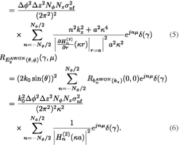
Before presenting the modal filtering, it is necessary to deter-mine the characteristics of the noise in each far-field component in order to obtain a reference with which to compare the results after the filtering process. These far-field components are ob-tained as described in [14] and the autocorrelation of the noise in each far-field component is

ñj BA W G N (9^ ) ( 7 , / i )

¿V¿/2

= (2k0sm(6))2 J ] i20AWGN(fe0(0,0)e^'í5(7)

Ac/>2Az2N^Nza2ní

( 2 T T2)2

x E

a „ ( 2 )

n=-Nt/2 \^g^{Kr)

n2k

*

+a2

«t e ^ (

7

) (5)

fiBAWGN(9W(7,/í)

r—a

¿V¿/2

(2fcosin(0))2 Y, ^AWGN(feí)(0,0)e^'í5(7) n = - i V0/ 2

fc02A«¿2Az2i\r^a2f

( 2 7 T2)2/ Í2

N+/2

x E i — —

n=-N^/2 \Hn '(na)

r e ^ ¿ ) (7) . ₍₆₎

As deduced from (5) and (6) and as was stated in [9], the autocorrelation of the far-field noise depends on 6 but not on <p. Therefore, the noise is nonstationary in elevation and stationary in azimuth. Moreover, the noise is white in 6 and colored in <fi because the autocorrelation is zero for 7 ^ 0 and nonzero for

\i ^ 0, respectively.

Up to now, a statistical study of the noise in the CNF to far-field transformation has been carried out. Although, this is not the main purpose of this work, the previous results provide useful information to achieve our objective, i.e., to be able to define a filtering to reduce the noise in the far-field pattern and to find the expression for the signal-to-noise ratio improvement. From (3) and (4), it was deduced that the noise is not sta-tionary but it is distributed over the whole n — kz domain. In

contrast, the desired information of the AUT is concentrated in the region specified in (1). Therefore, a filtering as defined in (7) can be applied to remove a portion of noise without cancelling the CMC which contain the AUT information:

F i n _ | l n2 + {kzaQ)2 < {kQa0)2 (visible)

n{ z) \ 0 n2 + {kza0)2 > (k0a0)2 (evanescent) '

(7)

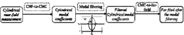
This filtering is depicted in Fig. 1 (a) and it is applied to the two sets of CMC. Once the evanescent modes has been filtered out, the noise in each far-field component is

E^r(o,4>)

N(e)

= 2fcosin(0) J2 .Ta£W G N(fcoCOS0)e^ (8)

n=-N(e)

N(6)

= -¿2fcosin(0) J2 Jnb^WGN(k0 cos e)e^ (9)

n=-N(e)

with

N(9) = ^(k0a0)2 - (kza0)2

= fcoao\/l — cos2(<?) = &oaosin(0). (10)

(a) Cb)

Fig. 1. Regions of interest used to define (a) the modal filtering and (b) the spatial filtering.

Therefore, the new autocorrelation of the far-field noise is

_ A4,2Az2NtNz*2ni X ? ( M ) ^ ' W - (2^2)2

N(e)

E

(2) n2kl + a2K4 -e^Si-t) (11)

N{8)

• E

n=-N{6)

k20A<j)2Az2Nt¡¡Nz(Tlt

( 2 7 T2)2K2

PJnf HÍ2\Ka)

5(7). (12)

The far-field noise obtained after the filtering process is also a Gaussian noise with zero mean, uncorrelated and nonstationary in 6, and correlated and stationary in <f>. When comparing (5) and (6) with (11) and (12) it is deduced that the only difference before and after applying the filtering is the number of terms in the summations. As deduced in (13), that number of terms is less or equal after the filtering stage.

Consequently, there is always a reduction of the noise power:

AT(0) = ^ a o s m ( 0 ) < ^

A0|r

2TT

(13)

Moreover, the modal filtering does not modify the AUT con-tribution. Therefore, the signal-to-noise ratio improvement can be calculated as the ratio between the noise power before and after applying the filtering:

ASNRE,(0)

fi£AWGN(9^(0,0)

# i ? A W G N( M )( 0 , 0 )

^ 2 n2k2 + a2^

E

n=-N</>/2

dHJ2) , s

- & i - ( «r)

N{9)

E

n2k2 +a2n4

(14)

\dH. (2)

ASNRBe (61)

n=-N(9) |i i^ - ( « x )

. R B A W G N ( 9 ^ ( 0 , 0 )

N+/2 i

^-^ (21 2

n=-N¿/2 H¿, '{na)

N{8)

E

n=-N(9)

(15)

Hi2\na)

Several conclusions can be extracted from (14) and (15). First, a different signal-to-noise ratio improvement is obtained for each far-field component. Second, the improvement is dependent on 0 but constant in <f>. Finally, the noise reduc-tion depends on the number of measurement points in <f>. i.e., depends on the azimuthal sampling spacing but not on the sampling spacing in z. As deduced from (5) and (6), a larger oversampling in z and <fi implies a smaller far-field noise variance, and consequently, a better signal-to-noise ratio. However, the signal-to-noise ratio improvement introduced by the modal filtering depends only on the oversampling in (p. In conclusion, an oversampling in both components introduces a signal-to-noise ratio improvement in the calculated far-field pattern, but when applying the modal filtering, a further noise reduction is achieved thanks to the oversampling in (p.

Next, simpler approximate expressions for the improvement achieved with this first filtering method are derived. Assuming that the argument values of the Hankel function and the derivate of the Hankel function are very large, the asymptotic expansion of these functions can be used instead:

\TTKaJ

1/2

dr (na)

•n+3/2K f_2_

\ 7 r / i a e

1/2

J «a ₍₁₆₎

(17)

The latter expressions constitute a good approximation when-ever na ^> 1. This condition is better fulfilled around 0 — 90° where K = fco- Moreover, the validity region of a CNF mea-surement is also around the horizontal direction. Therefore, the better approximation is given for the region of interest. Thus, it follows that (14) and (15) reduce to

ASNR£,(0) S

2 ^ 4

i2k2 + a~K 2nAa

Na

ASNR£ e (0)

N(9)

E

=-N(6)

N*/2

E

=-Nt/2

n2k2z + O2K4 2K4O

2N(6) (18)

TTKO,

~2~

NA N(9)

E

7TKO

~2~

2N{9) (19)

where the following approximation has been taken into account for the <j) component

, 2 7 . 2

fe, + a K = O K . ¿ i Z 4 r*j ¿ 4 (20)

Therefore, the improvement in both components is the same and is related to the sampling spacing in <f> as follows:

A ASNRfl,^) S NA

2N{0) 2A(j)a0 sin(0) Jav,(f)

A(/>sin(0) sin(ff) (21)

where it is deduced that the improvement is directly propor-tional to /ov,0, which is the oversampling factor in azimuth, and increases when we move away from the horizontal direction. Because the improvement is not a constant factor, the average signal-to-noise ratio improvement in the validity region can be considered as the figure of merit of this first filtering method:

7r/2+9„

ASNR.AV,modal

26v J sin(!

_ Jov,é 28,,

ir/2-0.

In

(*) dO

1 + sin(0„)

1 — sin(0„) (22)

where 8V is the maximum validity angle measured from the

hor-izontal direction.

Up to now, the signal-to-noise ratio improvement due to fil-tering has been evaluated with respect to the unfiltered case with the same sampling spacing. However, when comparing with the case without oversampling and without filtering, the improve-ment is as follows:

ASNIU-fiiW

Arh2 Az2 NJ. • N • NJ.

r m a x max T im m zim i n iV<p,min

/ov,

^2¿^z2N4,Nz

27r/A0max

2N{6)

2fcoOo sin(0)

/ o

JOV,0

:sin(0) ASNRov • ASNR

fii(0) (23)

where fOV}Z is m e oversampling factor in z and ASNRov

repre-sents the improvement due to the oversampling, which is only dependent on the oversampling in z, i.e., there is an improve-ment due to the oversampling whenever the oversampling is performed in z and there is an improvement due to the filtering whenever an oversampling in <j) is applied.

Finally, the main steps of this first filtering method are sum-marized. A schematic of the method is depicted in Fig. 2. As commented before, the CNF data are used to obtain the CMC. This data representation allows filtering out a portion of noise without canceling AUT information. Once the modal filtering has been applied, a far-field pattern with less noise power is obtained.

III. SPATIAL FILTERING METHOD

, ! CNF-loCMC

Cyiindncai *wdat

coefficient

-\ : Sfnji] filtering ; Filtered coefficients

.m.. Far-fiini ofia Ihtiwdol

Fig. 2. Schematic of the modal filtering method.

obtained from PNF measurements and consists of back-propa-gating the measured field from the scan surface to the plane of the AUT. In this new domain, the desired contribution is theo-retically concentrated in the antenna aperture, whereas the noise is spread over the whole reconstructed surface. Thanks to this fact, a spatial filtering may be applied, canceling the field lo-cated out of the AUT dimensions, which is only composed of noise.

As in the modal filtering method, a statistical analysis of the noise in this transformation is performed. Using acquired data containing only noise with the aforementioned statistical characteristics and applying a CNF-to-far-field transformation, the noise obtained in each far-field component is a complex Gaussian noise, with zero mean and autocorrelation given by (5) and (6). Once, the far-field components are known, an easy way to obtain the field distribution over the AUT plane is to calculate previously the plane wave spectrum (PWS), whose components are related to the extreme near-field of an antenna located in the xy-plane as indicated in (24):

^extreme^—y\X-> V) oo oo

= / f Px-y{kx,ky)e-ik'xe-ikyvdkxdky. (24) — oo —oc

Because in a CNF measurement the AUT is selected to be located in the yz-plane, the following change of coordinates is required before applying (24)

X — Vm j V — Zm) % — XTl (25)

where (xm,ym,zm) are the measurement coordinates and (x, y, z) represent the new coordinates used to calculate the

ex-treme near-field. Therefore, the x- and y-far-field components in the new coordinate system are

Finally, the PWS components needed in (24) can be calcu-lated as follows [1]:

*xy\Pmi *Pm)

_ *-Jx—y\"my *Pm)

jk0 cos(6) (28)

where 6 represents the elevation angle in the new coordinate system. Therefore, the autocorrelation of the noise in each PWS component is

flPAWGN(flmi¿m)(c,T)

= i 2£A W G N (9 m^m )( f , r ) cos

2(flTO)sin2(iftTO)

kl cos2(0)

J-R (r - \ C O s 2( ' /,r » )

+ % wG N ( 9 m > m )(i, T )f c o W w

flPAWGN(flmi¿m)(c,T)

= i ?£A W G N( 9 m^m )( ? , r ) sin

2(flm)

fc2cos2(0)'

(29)

(30)

From the two previous expressions, it is deduced that the noise in the PWS components is nonstationary both in 6m and (¡>m. Moreover, it is uncorrected in 9m and correlated in (¡>m.

However, that correlation in azimuth can be considered almost negligible. Thanks to this fact, the determination of the noise characteristics in the extreme near-field is simplified in a great way. The x- and y- components of the noise in the extreme near-field are calculated using the discrete versions of (24):

c1 iAWGN / s

extreme,x—y \ ' a )

Nk* N*y

= £ £ P ™ {^kyje-f-'e-**** (31)

a=l 6 = 1

where N^ and Nk are the number of samples of the PWS taken on a regular kx — ky grid. Because the PWS samples are known on a regular 8m — (f>m grid, and interpolation process is required. This interpolation introduces a correlation among samples, but as will be seen in Section IV, under certain con-ditions it is negligible and we can still assume that the noise is uncorrelated. Therefore, the autocorrelation of the noise in the extreme near-field can be easily calculated as shown (32):

Ex(8m,<pm) — Eym(6m,4>m)

= Egm(em,(j)m)cos(em)sm((j)m)

+ E^ cos(<£m) (26)

Ey(8m, 4>m) = EZm(8m, (f>m)

= -E9m{0m,<t>m)sm{6m) (27)

where (6m, (j>m) are the angular coordinates referenced to the

measurement coordinate system, in which the far-field pattern is known and EXm, EVm, Egm and E$m are the x-, y-, 6- and

^-far-field components in the measurement coordinate system, respectively.

fl^AWGN (X:y){X,£)

e x t r e m e , a : — y v l i f'

Nkjl Nky JV*„ Nky

= ££££*

a l = l 61 = 1 a 2 = l 6 2 = 1

x l / x - j / [kxal i kybl ) rx_y \kXa2 , Kyb2 ) \

. e-3k^al(X+X)e-3kybl{V+í)eJk^a2XeJkyb2y

Nkx Xky

=

££

ñ

P

Aw

„

GN

K,fcO(

0

'

0

)

a=l 6 = 1

From the previous expressions, it is deduced that the noise in the extreme near-field is correlated both in x and y. However, all the samples have the same noise power (autocorrelation for

X — £ — 0), i.e., the noise is stationary and is identically

dis-tributed over the whole reconstructed surface, whereas the de-sired field is theoretically concentrated in the aperture antenna. Therefore, a spatial filtering may be applied, canceling the field that is located out of the AUT dimensions and that is only com-posed of noise. This spatial filtering is defined in (33):

G{x,y) = 1 ÍÍAUT

o fi

R

-n

'AUT

(33)

where f i ^ and Í Í A U T represent the reconstructed plane and the AUT aperture depicted in Fig. 1(b).

Once the filtering has been described, an analysis to deter-mine the signal-to-noise ratio improvement is carried out. Be-cause the PWS and the extreme near-field are related by Fast Fourier Transforms, the Parseval's identity can be used to es-tablish a relationship between the noise powers in both domains. The relationship before applying the spatial filtering is given by (34):

N. Ny

a = l 6 = 1

NX Ny

Cylindrical HKWfiJÓ meosuremenl

Cilirtdricaí modal i'lffi-r.-f/nx

CMC-tcnfar-fieW :

Plane wave spectrin ofw \ht

sfjattaifitJenrjg

Filtered extrente

near-fiefd

; Spaliii ' I I ' V : in:.:

Extreme near-field

Far.fUtA pattern

F.'.T-IK-I^.ILV.

. i PWS

Plane novf

Fig. 3. Schematic of the spatial filtering method.

If now, (36) is divided by the total number of samples in both domains, the following result is obtained:

1 Nx Ny

~AT E E

R

p™

G

£

t

(*-. .*«) (°> °)

NxNy

* a=l 6 = 1

L-y,mt(k:ca'kyb>

N* Ny

*> x VI a=l 6 = 1

NxNy

(37)

where ÍAV.fiít a nd -PAV a r e the average noise power in the PWS

after and before applying the spatial filtering, respectively. Because the spatial filtering does not modify the desired in-formation (located within the AUT aperture), the last result can be employed to determine the average signal-to-noise ratio im-provement achieved with this second method:

•* * ' x y

^ E E ñ « ^ - > ^ ) ( 0 ' 0 ) (34) ASNRAV.spatiai

NxNy

* e t = l 6 = 1

PAV

DAV,fllt

NXNy

q

- ' Í Í A U T

(38)

where Nx and Ny are the number of samples in the

recon-structed plane, which are equal to the number of samples in the PWS, i.e., Nx = Nkx and Ny = Nky.

After applying the filtering, the relationship is as follows:

NX Ny

a = l 6 = 1

N. Ny

NXNy

" a=\ 6=1 N' N'

NxNy

" a=l 6 = 1

V V ñ£A W G N K , J / 6 ) (0'0)

* J * J extreme,a: — y \ a i !" '

(35)

where Í?PAWGN ik k \ is the autocorrelation of the noise in

^x-y,mt{K,ca.>Kyb)

the PWS after the noise filtering and Nx and N represent the

number of samples within the AUT aperture. As deduced in (32), all the samples in the extreme near-field have the same noise power. Therefore, the last equation can be simplified as (36) indicates:

NX Ny

a = l 6 = 1

NN, ' NX Ny

"EEv™^,y(°.

0

)' (

36

)

NxNy

" a = l 6 = 1

where SQR and SQAVT symbolize the area of the reconstructed

plane and AUT aperture, respectively. Although it seems we can obtained an infinite improvement by increasing the size of the reconstructed surface, there is a limitation that is related to the interpolation required in the process. A larger reconstructed sur-face implies a larger interpolation. Therefore, the PWS samples are more correlated and the previous samples in each measure-ment ring, i.e., the separation among analysis is no longer valid. This effect is analyzed in detail in Section IV.

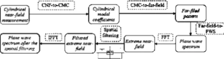
All the steps of this second filtering method are depicted in Fig. 3. The CNF data are used to obtain the far-field pattern by employing a modal expansion method. After that, the PWS components are calculated. Next, the extreme near-field is com-puted by means of a fast Fourier transform of the PWS. In this point, the spatial filtering defined in (33) is applied. Finally, a new PWS with less noise power is obtained by using an inverse fast Fourier transform.

IV N U M E R I C A L R E S U L T S

This section verifies the effectiveness of the proposed methods. The verification is carried out independently for each method by using both simulated and measured data.

A. Modal Filtering Method

(a) Maximum validity aaiiki^ raeir«s)

Fig. 5. Average signal-to-noise ratio improvement as a function of the max-imum validity angle and for different oversampling factors.

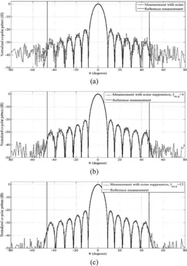
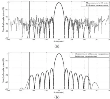
Fig. 4. Far-field comparison between (a) the reference pattern and the pattern with noise, (b) the reference pattern and the pattern after modal filtering with an oversampling factor equal to 4 and (c) the reference pattern and the pattern after modal filtering with an oversampling factor equal to 12 for the ¡j> = 0° cut.

acquisition. The AUT used in the simulation was a 8A x 8A aper-ture with a Gaussian-tapered field distribution. The frequency was 20 GHz, the samples were taken over a cylindrical sur-face of 3.38 m height (225 A), the radius of the cylinder was 1.5 m and the samples were spaced at 0.5A intervals in z. There-fore, two simulations with a different sampling spacing in <fi were performed. The first one took 288 samples was 1.25°. The second simulation recorded 900 samples per ring, i.e., the sam-pling spacing in azimuth was equal to 0.4°. Because the max-imum sampling spacing is 5.06°, the oversampling factor was approximately 4 and 12, respectively. Moreover, Gaussian noise with 38 dB less power than the maximum of the simulated data was added in both simulations. Next, the modal filtering method was applied. The far-field pattern without noise suppression as well as the far-field patterns obtained after the noise filtering are compared with the reference far-field pattern in Fig. 4. As de-duced in the theoretical analysis, the noise is more effectively reduced when the oversampling is greater. Fig. 5 shows the av-erage signal-to-noise ratio improvement defined in (22) as a function of the maximum validity angle and for different over-sampling factors. In our particular cases, where the maximum validity angle is 47.3°, the improvement is 6.58 dB for an over-sampling of 4 and 11.35 dB for an overover-sampling of 12. Fig. 6

Fig. 6. Exact and approximate signal-to-noise ratio improvement as a function of the elevation angle for an oversampling factor equal to 4 and 12.

depicts the exact improvement for both components calculated by using the expressions (14) and (15) and the improvement de-termined from the approximate expression given in (21) as a function of the elevation angle. Several conclusions can be ex-tracted from Fig. 6. First, the improvement is not constant in el-evation and increases when we move away from the horizontal plane. Second, the expression defined in (21) gives a better ap-proximation around the mentioned plane, which is the region of interest. Finally, the approximation is better for small values of the oversampling factor.

The second validation uses information from an actual mea-surement in the cylindrical near-field range of the Technical University of Madrid (UPM). For the experiment, the probe and the AUT consisted of a corrugated conical-horn antenna and a Ku-band reflector (14 GHz), with a 40 cm diameter, respec-tively. The data were acquired over a cylinder with a height of

1.8 m and a radius of 0.63 m and with a spatial sampling equal to 0.5A in the vertical direction and 0.375° in azimuth. Because the maximum sampling spacing in azimuth is 3.06°, the over-sampling factor was approximately 8. After measuring the AUT, Gaussian noise with 42 dB less power than the maximum of the acquired data was computationally added. The noise power was chosen to be large, so as to ensure a negligible measurement noise. The far-field obtained from the measured data without additive noise can thus be used as a reference to compare re-sults before and after noise filtering. The far-field rere-sults ob-tained before and after applying the filtering are compared with the reference pattern in Fig. 7. According to (22) and Fig. 5, the average improvement was 9.61 dB.

B. Spatial Filtering Method

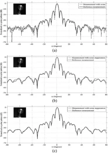
Fig. 8. Far-field comparison between (a) the reference pattern and the pattern Fig. 7. Far-field comparison between (a) the reference pattern and the pattern w i t h n°ise> (b)t h e reference pattern and the pattern after spatial filtering for the

with noise and (b) the reference pattern and the pattern after modal filtering with 9> = 0 cut. an oversampling factor equal to 8 in the horizontal plane.

second method, an oversampling in azimuth is not required, as deduced in the theoretical analysis. Therefore, the sampling spacing in azimuth used in the simulation is equal to the max-imum sampling spacing, i.e., 3°. Moreover, Gaussian noise with 30 dB less power than the maximum of the simulated data was added, instead of a noise with 38 dB less power. The objec-tive of increasing the noise power is to demonstrate that with this second method is possible to obtain a larger improvement using even a less number of acquired data. Once the new cylin-drical acquisition was simulated, the extreme near-field was de-termined over a square plane of 225A side, which was equal to the height of the measurement cylinder. After that, a spa-tial filtering was applied, canceling the field that was located out of the AUT dimensions and that was only composed of noise. Finally, the filtered field distribution was inverse Fourier transformed back to the spectral domain, obtaining a new far-field pattern where the noise power was greatly reduced, as ob-served in Fig. 8. The average signal-to-noise ratio improvement achieved in this case was, according to (38), 28.98 dB. Theoret-ically, with this method we can always increase the signal-to-noise ratio by using a larger reconstructed surface. However, this statement is not completely true because of the interpolation required in the spectral domain. A larger reconstructed surface implies a smaller sampling spacing in the PWS, i.e., more sam-ples have to be interpolated from the known samsam-ples. Therefore, the correlation among noise samples increases and the assump-tion employed in (32) is no longer valid. As a result, the noise in the extreme near-field is nonstationary, decreasing from the center to the edges of the reconstructed plane. Consequently, the noise reduction in the filtering process is not as effective as when the noise is stationary. This effect is depicted in Fig. 9, where the theoretical improvement defined in (38) is compared with the improvement observed in different examples with different

-Oh*orv«IASMnTAt-lDjuid 1^-ICO?. - UlWvvtl aSNK^at-1.5 • imd I.- LOU?. -OI»»TVíd.lSNR,í\4~.V 3diLl lv- 2 ; i ? . -Ob»mv»d¿SNRTA+-l.5'»nd L-235Í.

Fig. 9. Theoretical and observed average signal-to-noise ratio improvement for different acquisition parameters as a function of the size of the reconstructed surface.

acquisition parameters. As deduced from Fig. 9, when reducing the spatial sampling in <p or when increasing the height of the measurement cylinder, the improvement is larger for the same size of the reconstructed surface because, in both cases, we are reducing the spacing among known samples in the PWS, and a less number of samples have to be interpolated. Moreover, once the size of the reconstructed surface is larger than the height of the cylinder, the improvement remains constant. Due to this ef-fect, the improvement is not 28.99 dB but 20.20 dB, which is the maximum achievable with a spatial sampling in <j) equal to 3° and a height of the measurement cylinder equal to 225A.

(a)

(b)

Fig. 10. Far-field comparison between (a) the reference pattern and the pattern with noise, (b) the reference pattern and the pattern after spatial filtering on the AUT aperture, and (c) the reference pattern and the pattern after spatial filtering on a larger surface in the horizontal plane.

to be concentrated on the AUT region. Nevertheless, this as-sumption is not completely correct. A small field contribution always exists outside the AUT. Due to this fact, when using a filter with the same size as the AUT aperture, a portion of desired signal is canceled. This cancellation introduces an error in the side-lobes of the reconstructed far-field pattern around ±60°, as observed in Fig. 10(b). To avoid this negative effect, spatial fil-tering over a larger area must be employed to account for all of the desired data. However, this new filter integrates more noise power. Therefore, a compromise is required between the noise reduction and an accurate far-field representation. In this partic-ular case, a filtering window with a size one and a half times the size of the antenna aperture was also employed. The improve-ment achieved with this filtering is 10.06 dB, which is smaller than that one obtained with the filtering of minimum size. How-ever, because more information about field radiated by the AUT is not filtered out, the reference pattern is better retrieved, as it is possible to see in Fig. 10(c).

V CONCLUSION

Two simple and efficient methods to improve the signal-to-noise ratio in the far-field results obtained from cylindrical near-field measurements were presented. The first method applies a filtering in the modal domain and its main

drawback is the necessity of oversampling, increasing the measurement time. However, this is not a critical aspect when measuring in a multi-probe system. Moreover, it is possible to improve the signal-to-noise ratio in all directions. The second method employs a source reconstruction technique to filter out the noise in the extreme near-field. Unlike the modal filtering method, this second approach does not require an oversam-pling. In addition, a better improvement is obtained using less measured data because of the use of more a priori information about the AUT. Whereas in the modal filtering, only infor-mation about the size of the AUT is required to defined the visible region, in the spatial filtering method both the size and the exact position of the antenna need to be known. Moreover, the spatial filtering method only provides a noise reduction in the forward hemisphere and it was noted that works better for planar aperture antennas because the region, in which the fields are assumed to be concentrated, is well defined. In contrast, the modal filtering method is independent of the shape of the antenna and it can be applied to antennas with arbitrary geome-tries obtaining similar improvements. Approximate theoretical expressions were derived for the improvement achieved with both methods. Finally, these expressions as well as the effec-tiveness of the methods were verified through application to both simulated and measured near-field data.

REFERENCES

[i]

[2]

[3]

[4]

A. D. Yaghjian, "An overview of near-field antenna measurements,"

IEEE Trans. AntennasPropag., vol. AP-34, no. 1, pp. 30-44, Jan. 1986.

R. C. Johnson, H. A. Ecker, and J. S. Hollis, "Determination of far-field antenna patterns from near-field measurements," Proc. IEEE, vol. 61, no. 12, pp. 1668-1694, Dec. 1973.

P. Petre and T. K. Sarkar, "Planar near-field to far-field transformation using an equivalent magnetic current approach,"ZEEE Trans. Antennas

Propag., vol. 40, no. 11, pp. 1348-1356, Nov. 1992.

A. C. Newell, "Error analysis techniques for planar near-field measure-ments," IEEE Trans. Antennas Propag., vol. 36, no. 6, pp. 754-768, Jun. 1988.

[5] L. A. Muth, "Displacement errors in antenna near-field measurements and their effect on the far-field," IEEE Trans. Antennas Propag., vol. 36, no. 5, pp. 581-591, May 1988.

[6] J. E. Hansen, "Error analysis of spherical near-field measurements," in

Spherical Near-Field Antenna Measurements. London, U.K.: Peter

Peregrinus, 1988, ch. 6, pp. 216-254.

A. C. Newell and C. F. Stubenrauch, "Effect of random errors in planar near-field measurement," IEEE Trans. Antennas Propag., vol. 36, no. 6, pp. 769-773, Jun. 1988.

J. B. Hoffman and K. R. Grimm, "Far-field uncertainty due to random near-field measurement error," IEEE Trans. Antennas Propag., vol. 36, no. 6, pp. 774-780, Jun. 1988.

[9] J. Romeu, L. Jofre, and A. Cardama, "Far-field errors due to random noise in cylindrical near-field measurements," IEEE Trans. Antennas

Propag., vol. 40, no. 1, pp. 79-84, Jan. 1992.

[10] J. Romeu and L. Jofre, "Effect of random errors in cylindrical near-field measurements," in Proc. IEEE/APS Int. Symp., London, ON, Canada, Jun. 24-28, 1991, pp. 1450-1453.

P. Koivisto, "Reduction of errors in antenna radiation patterns using optimally truncated spherical wave expansion," Progress In

Electro-magn. Res., vol. PIER-47, pp. 313-333, 2004.

L. J. Foged and M. Faliero, "Random noise in spherical near-field sys-tems," inProc. AntennaMeas. Tech. Assoc, AMTA, Salt Lake City, UT, Nov. 1-6, 2009, pp. 135-138.

[13] F. J. Cano-Fácila, S. Burgos, and M. Sierra-Castafler, "Novel method to improve the signal-to-noise ratio in the far-field results obtained from planar near-field measurements," IEEE Antennas Propag. Mag., vol. 52, no. 2, pp. 215-220, Apr. 2011.

[14] O. M. Bucci and C. Gennarelli, "Use of sampling expansions in near-field-far-field transformations: The cylindrical case," IEEE Trans.

An-tennas Propag., vol. 36, no. 6, pp. 830-835, Jun. 1988.

[7]

m

in]

[15] A. D. Yaghjian, "Near-field antenna measurements on a cylinder sur-face: A source scattering matrix formulation," Nat. Bur. Stand. NBS Tech. Note 696, July 1977.

[16] S. Gregson, A. Newell, and G. Hindman, "Reflection suppression in cylindrical near-field antenna measurement systems-cylindrical MARS," in Proc. Antenna Meas. Tech. Assoc, AMTA, Salt Lake City, UT, Nov. 2009, pp. 119-125.

[17] G. E. Hindman and A. Newell, "Reflection suppression in a large spher-ical near-field range," in Proc. Antenna Meas. Tech. Assoc, AMTA, Newport, RI, Oct. 2005.

[18] D. W. Hess, "The IsoFilter™ technique: Extension to transverse off-sets," in Proc. Antenna Meas. Tech. Assoc, AMTA, Austin, TX, Oct. 2006.

[19] S. Gregson, A. Newell, G. E. Hindman, and M. J. Carey, "Extension of the mathematical absorber reflection suppression technique to the planar near-field geometry," in Proc. Antenna Meas. Tech. Assoc,

AMTA, Atlanta, GA, Oct. 2010.

[20] S. Gregson, B. M. Williams, G. F. Masters, A. Newell, and G. E. Hindman, "Application of mathematical absorber reflection suppres-sion to direct far-field antenna range measurements," in Proc. Antenna

Meas. Tech. Assoc, AMTA, Denver, CO, Oct. 2011.

[21] O. M. Bucci, G. D'Elia, and M. D. Migliore, "A general and effec-tive clutter filtering strategy in near-field antenna measurements," IEE

Proc. Microw., Antennas, Propag., vol. 151, no. 3, pp. 227-235, Jun.

2004.

[22] W. M. Leach and D. T. Paris, "Probe compensated near-field measure-ments on a cylinder," IEEE Trans. Antennas Propag., vol. AP-21, no. 4, pp. 435^145, Jul. 1973.

antenna measurement, focusing specifically on diagnostics techniques and near-field to far-near-field transformations.

Dr. Cano-Fácila was awarded the highest marks for the telecommunication engineering degree in 2007. He obtained his M.Sc. degree with special distinc-tion and was awarded a Ph.D. scholarship from the Spanish government. He also obtained the first place, AMTA student paper contest, for the paper titled "Novel method to improve the signal to noise ratio in the far-field results obtained from planar near-field measurements" presented in Atlanta in October 2010.

Manuel Sierra-Castañer (S'95-M'Ol) was born in

Zaragoza, Spain, in 1970. He received the degree in telecommunication engineering and the Ph.D. degree from the Technical University of Madrid (UPM), Madrid, Spain, in 1994 and 2000, respectively.

He worked for Airtel, a cellular company, from 1995 to 1997. Since 1997, he has worked in the Uni-versity "Alfonso X" as an Assistant Professor. Since 1998, he has worked at the Technical University of Madrid as a Research Assistant, Assistant Professor, and Associate Professor. His current research inter-ests involve planar antennas and antenna measurement systems.

Dr. Sierra-Castañer obtained the IEEE APS 2007 Schelkunoff Prize for his paper "Dual-Polarization Dual-Coverage Reflectarray for Space Applications" in 2007.

Francisco José Cano-Fácila was born in Don

Benito, Spain, in 1985. He received the M.Sc. degree in telecommunication engineering and the Ph.D. degree from the Technical University of Madrid, Madrid, Spain, in 2008 and 2012, respectively.