Technical efficiency of Spanish construction sector pre- and
post-housing bubble burst
Xosé Luís Fernández López,
Pablo Coto-Millán
Santander, September 2013
MÁSTER EN ECONOMÍA, INSTRUMENTOS DE ANÁLISIS
ECONÓMICO
Abstract: The main objectives of this paper are to measure the technical efficiency levels of Spanish construction sector before and during the current financial crisis and to investigate the degree to which various factors influence efficiency levels in this sector. Stocastic frontier analysis (SFA) methods are applied to firm-level data over the period 1996-2011. Despite its contribution to the Spanish economy the technical efficiency of the Spanish construction industry has neither been measured, nor the factors influencing the efficiency have been analyzed.
The results show that technical efficiency is significantly shorter at the beginning of the financial crisis than during the financial crisis. Results also show that firms that went bankrupt, on average have a lower technical efficiency level than firms that did not go bankrupt in the period before the Spanish housing bubble burst.
We also identify several important factors affecting technical efficiency levels. Our empirical results indicate that age, size, level of diversification, level of corporate transparency an level of debt have a significant influence on technical efficiency levels.
1. Introduction.
The concept of “construction” is unusually complex. It brings problems of quantifying output, of value-added, of relative prices, etc. Almost every project in construction is unique, and it is exceedingly difficult to find a uniform measure of the quality of construction projects.
The Construction Sector is both highly competitive and cyclically sensitive (Moscarini and Postel-Vinay 2009). The short term supply is inelastic in the sector thereupon increases in demand produce rapid increases in prices. This one of the main reasons why construction companies commonly operate with a high level of financial leverage leading to the exposure of financial stress and continuous liquidity problems as a result of financial markets movements.
Buildings, heavy civil and specialty trade are the construction main activities ( I. M. Horta et All,2012). The construction of buildings and civil engineering works is undertaken in a similar way worldwide: a general contractor, responsible for delivering the finished project to the owner, subcontracts much of the practical work to specialty trade companies. The building segment includes the general contractors, who build residential buildings, and nonresidential, such as industrial, commercial, and other buildings. Residential building companies are associated with household demand.
The real estate bubble formation is linked to three intrinsic characteristics of the construction and real estate activities: rigid supply in the short term, important role of expectations for supply and demand, and high leverage on production and home purchase.
During the decade of 1997-2006 Spain has been featured in the formation of a real estate bubble. The Spanish construction sector enjoyed a period of constant growth, reaching a 12.1% share of gross value added in 2006, which is twice the overall comparable figure for the EU, and employing 2.8 million persons (13% of the labor force in 2007). Until 2007, Spain was recording higher annual new home construction completions than France, Germany and Italy combined. However, we should note that the formation of a real estate bubble has not been just a Spanish issue and the United States, UK, Ireland, South Africa, China, and Argentina, among others, have attended the formation of this phenomenon. But Spain is highlighted as one of the countries most affected after the bursting of the bubble.
Unleashed in 2007 by the burst of the Spanish Housing Bubble the financial crisis unfolded at a speed and magnitude even the most die-hard pessimists could not have predicted. Because of the cyclical nature of the construction industry the situation had been more adverse
to construction firms than to other firms. A drastic decrease in demand for new housing added to the high external debt that the companies suffer from cause the wholesale collapse of its industry. As an example, the number of licenses authorized for the construction of buildings issued in 2011 only account for fourteen percent of those issued in 2006 (Spanish National Statistics Institute). A great number of bankruptcies among Spanish construction firms, that failed to adapt themselves to the changing environments, including some major construction firms such as, Astroc Mediterraneo, Martinsa-Fadesa, Habitat, and most recently Reyal Urbis, all characterized by a high external debt and extremely exposed to real estate business.
And yet here Spain has today the largest construction sector among the EU countries (Eurostat, GVA 2010). The Spanish construction sector supported in the internationalization reaches to the second place in the ranking of constructions companies elaborated by Deloitte (European Powers of Construction). The construction industry is no longer a local market, given globalization. The global construction industry makes up approximately 9% of the world’s GDP. This sector is the largest industrial employer in most countries, accounting to around 7% of the total employment worldwide (I. M. Horta et al, 2012). Construction companies are adopting strategies of internationalization that enable them to benefit from the global market. In particular, some Spanish construction companies have moved their entire operations to Latin America, Southeast Asia, and the Middle East, with lower running costs, more work and opportunities.
Despite its contribution to the Spanish economy the technical efficiency of the Spanish construction industry has neither been measured, nor the factors influencing the efficiency have been analyzed. Globally, country studies report a wide range of efficiency levels. These range from a low of around 50% for Canadian firms (Pilateris and McCabe, 2003), 57% for Vietnamese firms (Nguyen and Giang, 2005), approximately 60% for Portuguese firms (Horta et al., 2012), to higher estimates of 83% for Norwegian firms (Edvardsen, 2004) and 93% for Greek firms (Tsolas, 2011).
Interesting because of the resemblance to the Spanish case, is the study of You and Zi (2007), in which analyzed the case of Korea in the late 1990’s. The Korean construction sector was impacted by an economic crisis in November 1997. Using a data envelopment analysis (DEA) approach for the period 1996-2000, the author focus on leverage ratio, export weight, institutional ownership, asset size and receivables overdue turnover and find these factors impact all efficiency measures.
Other studies that should be emphasized on the construction field are Horta et al., 2010 and El-Mashaleh et al.,2011, where author’s use the DEA method to evaluate the safety efficiency of every contractor aiming to transform inefficient contractors into high efficiency contractors.
In this article we gauge and analyze the technical efficiency of the Spanish Building industry for the period 1996-2011.
2. Literature review
The technical efficiency of a production may be defined as the ability of a firm to produce as much output as possible given certain levels of inputs or factors of production, and certain technology.
Farrell (1957) suggested a method of measuring the technical efficiency of a firm in an industry by estimating the production function of firms which are “fully-efficient”.
We will take as given the existence of a well-defined production structure characterized by smooth, continuous, continuously differentiable, quasi-concave production or transformation function. Producers are assumed to be price takers in their input markets, so input prices are treated as exogenous. The empirical measurement of TE(y,x) requires definition of a transformation function
Let
( )
y f x (1.0)
denote the production function for the single output, y, using input vector x. Then, an output based Debreu-Farrell style measure of technical efficiency is
( ) = 1. ( ) y TE y, f x x (1.1)
Farrell suggested that one could usefully analyze technical efficiency in terms of realized deviations from an idealized frontier isoquant. This approach falls naturally into an econometric approach in which the inefficiency is identified with disturbances in a regression model.
Many subsequent papers have applied and reviewed Farrell’s ideas. This literature may be roughly divided into two groups according to the method chosen to estimate the frontier
production function, namely, Deterministic Frontier versus Stochastic Frontiers. Debate continues over which approach is the most appropriate method to use. The answer often depends upon the application considered.
4.a. Deterministic Frontiers
Fallowing (Ruggiero, 2007), we assume N producers that faces the same production technology represented by the conversion of a vector X of inputs into a single outputy. For simplicity, we assume that efficient production can be represented by a Cobb–Douglas production function with two inputs
y
= AX
11
X
22
(1.3)
This production function, showing the maximum output from given input usage, will serve as the basis for efficiency measurement. Allowing inefficiency, we can represent (1.3) with the empirical production function
y
= AX
11
X
22
u (1.4)
where u 1 represents inefficiency. Models that seek to estimate u based on (1.4) are considered deterministic because measurement error and other statistical noise are assumed away.
Taking Greene method (GM) (Greene, 1980), the production function can be estimated by taking logs and using OLS as
ln 1ln 1 2ln 2 lny a b x b x (1.5) Greene proved that OLS produces consistent estimates for the slope parameters. The largest positive residual is added to the intercept and subtracted from the residuals. Hence, the adjusted residual represents the shortfall in output from the efficient level. Given the resulting residuals i for observation i, efficiency is estimated as
j
j
i
ˆexp( max
Because of the needed of a priori specification of the production function in GM, the most widely used deterministic approach is not the GM but Data Envelopment Analysis (hereinafter DEA). DEA is a non-parametric approach -it does not require any assumption about the functional form of the production or cost frontier- introduced by Charnes et al.
(1978) to measure efficiency under the assumption of constant returns to scale, and extended by Banker et al. (1984) to allow variable returns to scale.
Advantages of the DEA approach are the nonparametric nature and the ability to handle multiple outputs and multiple inputs. As disadvantages, econometricians have argued that the approach produces biased estimates in presence of measurement error and other statistical noise.
The lack of allowance for statistical noise is widely regarded as the most serious limitation of DEA, because this puts a great deal of pressure on users of this technique to collect data on all relevant variables and to measure them accurately. The following two issues, however, have been frequently ignored despite their importance.
DEA is the solution to the fallowing mathematical problem
j j ko o N j kj j N j j j o o
k
x
x
y
y
T
S
Min
o
, 0 1 · 1 ·2
,
1
:
,
.
.
ˆ
(1.6)where subscript ‘o’ represents the firm under analysis. DEA requires solving program (1.6) for each of the N producing units. Solution for all decision-making units leads to a vector ˆCCR of
efficiency estimates. Adding the convexity constraint
N j 1j 1 to (1.6) results in the variable
returns to scale DEA model of Banker et al. (1984).
A potential problem in the comparison of DEA and other approaches is the excess slack that may exist in some but not all of the input constraints. As a result, the equi-proportional estimate ˆCCR may not capture all inefficiency. Therefore, we also consider the alternative
j j ko ko N j kj j N j j j o o rok
x
x
y
y
T
S
Min
o
, 0 1 · 1 · 2 12
,
1
:
,
.
.
*
5
.
0
ˆ
(1.7)The solution of (1.7) for a given decision-making unit results in a non-proportional efficiency estimate and reduces the problem of (1.6) with excess input slack. Solution for all decision-making units leads to a vector ˆRussell of efficiency estimates.
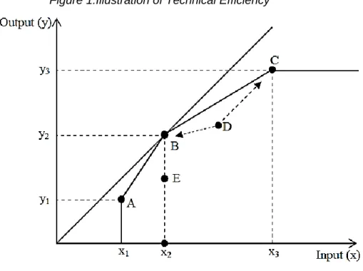
Figure 1 illustrates this definition. In the figure, there are five points (A–E) associated with different levels of input and output. The line ABC describes the frontier for the production process. Observations A, B, and C are on the frontier, while observations D and E lie below the frontier. There exists a ray from the origin tangent to the frontier at point B representing the constant returns to scale of the technology. In this example, observation B represents the relative technical efficiency, whereby this firm is technically and scale efficient because of its location on the frontier and the property of constant returns to scale.
As it can be seen in Figure 1 (observations A and C), in an overall sense, a firm could be technically efficient, while experiment inefficiency in scale. Namely A and C are purely technically efficient because they belong to the frontier, but they exhibit scale inefficiencies.
Instead, observation D is both scale and technically inefficient because it lies below the frontier. Theoretically, the same level of input could be used to achieve a higher level of output, which will allow this firm (at point D) to move forward to the frontier between points B and C.
Observation E is technically inefficient because it lies below the frontier, but it is scale efficient because it produces at input level of , the same level of output as observation B.
Figure 1:Illustration of Technical Efficiency
Deterministic approaches are based in cross-sectional models; however, they can be extended to panel data models by averaging the data across time. Ruggiero (2004)
Recently, data envelopment analysis has become the dominant approach to measure the performance of many economic sectors. One of the attractive characteristics of DEA is that it can deal with multiple outputs easily.
4.b. Stochastic Frontiers
The stochastic production frontier is motivated by the idea that deviations from the production ‘frontier’ might not be entirely under the control of the firm being studied. Under the interpretation of the deterministic frontier of the preceding section, for example, an unusually high number of random equipment failures, or even bad weather, might ultimately appear to the analyst as inefficiency.
Since Aigner, Lovell, and Schmidt proposed their pioneer work in 1977, both the theoretical development and empirical application of stochastic frontier models have prospered in the literature.
A more appealing formulation holds that any particular firm faces its own production frontier, and that frontier is randomly placed by the whole collection of stochastic elements which might enter the model outside the control of the firm.
( ) vi
i i i = f
y x TEe ,i=1,...,N, (1.8)
where TEi corresponds to , and vi is unrestricted. The latter term embodies measurement
errors, any other statistical noise, and random variation of the frontier across firms. The reformulated model, taking on log-linear (Cobb-Douglas) production function, is
ln yi =o +
k j 1 j xji+ (vi - ui) = o +
k j 1 j xji + ,i=1,...,N, (1.9)As before, ui > 0, but vi may take any value. A symmetric distribution, such as the normal
distribution, is usually assumed for vi. Thus, the stochastic frontier is o + j xji+ vi and, ui
represents the inefficiency.
Discussions about the distribution of the compound disturbance in the stochastic frontier model have been done. The literature begins with Aigner, Lovell and Schmidt’s (1977)
Normal-half normal model, where
ui = |Ui| where fU(Ui) = N[0,u2] = (1/u)(Ui/u), - < Ui < , (1.10)
Stevenson (1980) introduce the Truncated normal model arguing that the zero mean assumed in the Aigner, et al. (1977) model was an unnecessary restriction. He produced results for a truncated as opposed to half-normal distribution. That is, the one-sided error term, is obtained by truncating at zero the distribution of a variable with possibly nonzero mean.
The log-likelihood function for each of the two models, have been derived, and has been integrated into several commercial computer packages, starting with Frontier4 (Coelli (1996)), LIMDEP (Greene (2000)), and incorporated at the present time into free software including Gretl and R.
A variety of specifications of the model production and (in)efficiency have emerged during this time as alternatives to the production frontier. Among them:
Stochastic frontier cost functions. Introduce a distinct representation of the production technology, under a set of regularity conditions (Shephard (1953)). In the construction sector, a recent paper of Dzeng, R. et al. ( 2013) used the stochastic frontier analysis to model and measure the cost efficiency of construction firms in Taiwan.
Multiple outputs production/cost functions. As an example of multiple production
function see Fernandez et al. (2000). The authors use an output aggregator that links the
k
‘aggregate output’ to a familiar production function. See Orea and Kumbhakar (2003), as an example of cost function in the Spanish bank sector.
Another approach that has proved useful in numerous empirical studies is the Distance
and profit function, based in Shephard's input distance function.
Panel data applications have kept pace with other types of developments in the literature. A fundamental question concerns whether inefficiency is properly modeled as fixed over time. Intuition should suggest that the longer is the panel, the ‘better’ will be the estimator of time invariant inefficiency in the model, however computed. But, at the same time, the longer is the time period of the observation, the less tenable the assumption becomes (Greene, 2005). Treatments of firm and time variation in inefficiency are usefully distinguished in two dimensions. The first is whether we wish to assume that it is time varying or not. Second, we consider models which make only minimal distributional assumptions about inefficiency (‘fixed effects’ models) and models which make specific distributional assumptions such as those made earlier, half normal, exponential, etc.
Pitt and Lee (1981), Kumbhakar’s (1990), Lee and Schmidt (1993) Battese and Coelli’s (1992) suggested different Stochastic Panel Data Models.
The debate on whether to use one-step or two-step approach brought important developments in the investigation of how exogenous factors influence the one-sided inefficiency effect. This effort allows researchers to understand not only the production unit’s state of efficiency, but also the contributing factors of the efficiency. As an argument in favor of one-step approach it is easy to think that not accounting for the exogenous influences at the first step will induce a persistent bias in the estimates that are carried forward into the second. The extensive Monte Carlo results presented by Schmidt and Wang (2002) give evidence in favor of the one-step approach.
Perhaps the most well-known model of the one-step approach is the Battese and Coelli (1995) Model. These authors propose parameterizing the mean of the pre-truncated distribution as a way to study the exogenous influence on inefficiency.
Heterogeneity was another topic of discussion among researchers. Greene, 2004 categorize heterogeneity between observable and unobservable heterogeneity. The parameters of the underlying distribution of ui provide a mechanism for introducing heterogeneity into the
distribution of inefficiency. The mean of the distribution (or the variance or both) could depend on factors such as industry, location, capital vintage, and so on. In Orea et al. (2004)
and Greene (2005), a latent class specification is suggested to accommodate heterogeneity across firms in the sample.
Recent research works try to combine strengths of stochastic method into DEA Models. As an example Simar et al, 2011 integrate a stochastic SFA-style noise term to the nonparametric, axiomatic DEA-style cost frontier.
Ruggiero, 2007, using simulated data, compare DEA and SFM and show: Firstly, Additional time periods improve the performance of all measures. Secondly, as the variance of the measurement error term increases holding the number of periods fixed the performance of all estimators’ declines on average. Third, in almost all cases, the stochastic frontier model outperforms the other measures.
Badunenko, Henderson and Kumbhakar (2012) show that the reliability of efficiency scores hinges critically on the ratio of the variance of inefficiency to the variance of noise; with high ratio, both methods work well; with medium ratio, both methods underestimate efficiency but SFA does so by less; with low ratio, both methods perform poorly.
3. Teorical Model
To measure the efficiency for the of Spanish construction sector and identify explanatory variables of the (in)efficiency, we propose the Stochastic frontier production
function for unbalanced panel data developed by Battese and Coelli (1992), and the Technical inefficiency effects model Battese and Coelli (1995) . As we have seen in section 2, this type of
frontier and the computation method present advantages with respect other alternatives. For example the mathematical programing (DEA) are extremely sensitive to the existence of outliers. As well, the estimated coefficients of DEA method lack statistical properties (statistical inference, hypothesis contrasts,...).
In the other hand, the function that explains the inefficiency scores is estimated in a single stage with the production technology, which avoids the problem of inconsistency that the two stage approach suffers from, Wang (2002).
Following Battese and Coelli (1992), the stochastic frontier production function proposed, has firm effects that are assumed to be distributed as truncated normal random variables and, also, are permitted to vary systematically with time. The model may be expressed as:
Yit =o +
k
j 1
j Xjit+ (Vit - Uit) ,i=1,...,N, t=1,...,T, (3.1)
where Yit denotes (the logarithm of) the production of the i-th firm in the t-th time period; Xk
represents the k-th (transformations of the) input quantities; k stands for the output elasticity
with respect to the k-th input; the Vit is a random variable which is assumed to be iid N(0,V2),
and distributed independently of the Uit which has the specification:
Uit = Uiit = Uiexp(-(t-Ti)) (3.2)
where the Ui is a non-negative random variable which is assumed to account for technical
inefficiency in production and are assumed to be iid as truncations at zero of the N(,2)
distribution and is a parameter to be estimated.
The last period (t=Ti) for firm i contains the base level of inefficiency for that firm (Uit
= Ui). If > 0, then the level of inefficiency decays toward the base level. If < 0, then the
level of inefficiency increases to the base level, and if = 0, then the level of inefficiency
remain constant.
Using the parametrization of Battese and Corra (1977) who replace V2 and 2 with
2
=V2+2 and =2/(V2+2). The parameter , must lie between 0 and 1.
The imposition of one or more restrictions upon this model formulation can provide a number of special cases of this particular model, which have appeared in the literature. For example, setting to be zero provides the time-invariant model. One can also test whether any form of stochastic frontier production function is required at all by testing the significance of the parameter. If the null hypothesis, that equals zero, is accepted, this would indicate that
2 is zero and hence that the Uit term should be removed from the model, leaving a
specification with parameters that can be consistently estimated using ordinary least squares. The predictions of individual firm technical efficiencies from the estimated stochastic production frontiers are defined as:
EFit= exp(-Uit)= E[exp(-Uit)Ei] =
* 2 *2 * * * * * 2 1 exp / 1 ) / ( 1 i it i i i i i i it it (3.3)where Ei represents the (Ti x 1) vector of Eit ‘s associated with the time periods observed for the
2 2 2 2 i i V i i V i E ' ' * (3.4) 2 2 2 2 2 i i V V i ' * (3.5)
where i represents the (Ti x 1) vector of it ‘s associated with the time periods observed for the
i th firm, and (.) represents the distribution function for the standard normal random variable.
If the firm effects are time invariant, then the technical efficiency is obtained by replacing it =
1 and = 0.
The main objective of this study is to provide measures of technical efficiency ant to identify explanatory variables that may help explain some of the technical efficiency variations. It has been utilized a Technical inefficiency effects model (TIE), Battese and Coelli (1995). In this model the function that explains the inefficiency scores is estimated in a single stage with the production technology, which avoids the problem of inconsistency that the two stage approach suffers from.
Then, Ui is assumed to account for technical inefficiency effect in production and are
also assumed to be iid as truncations at zero of the N(,2).
Uit = zit δ +Wit (3.6)
zit, is a (1 x m) vector of explanatory variables associated with technical inefficiency of
production of firms over time. The explanatory variables may include some input variables in the stochastic frontier, provided the inefficiency effects are stochastic. If the first z-variable has value one and the coefficients of all other z-variables are zero, then this case represents the model specified in Stevenson (1980) and Battese and Coelli (1992).
δ is an (m x 1) vector of unknown coefficients. If all elements of the δ -vector are equal
to zero, then the technical inefficiency effects are not related to the z-variables and so the half-normal distribution originally specified in Aigner, Lovell and Schmidt (1977) is obtained.
Wit is random variable N(0,2), but not necessarily identically distributed.
Uit non-negative truncation of the N(zit δ,2) distribution. The mean zit δ of the normal
distribution, which is truncated at zero to obtain the distribution of Uit, is not required to be
positive for each observation.
The technical efficiency of production for the i-th firm at the t-th observation is defined by equation: TE it, = exp( -U it) = exp( - zit δ - Wt,). The method of maximum likelihood is
proposed for simultaneous estimation of the parameters of the stochastic frontier and the model for the technical inefficiency effects.
4. Data and Empirical specification.
The SABI (Sistema de Análisis de Balances Ibericos) database, managed by Bureau van Dijk, provides the necessary data to estimate an efficiency measure. The study sample includes the firms belonging to the category of firms in, Real estate development, Construction of residential buildings, Construction of non-residential buildings (NACE Rev. 2 codes 4110, 4121, 4122). The database is an unbalanced panel observed over the period 1996-2011. SABE also provides information about the major two-digit NACE codes to which the firms belong.
Table 1 reflects the sectorial division of the service sector analyzed in this paper, the number of firms and the number of observations of each subsample.
Table 1: Sector classification, number of firms and number of observations
CNAE Sector classification Num.of firms Num.of
observations
4110 Real estate development 472 3804
4121 Residential buildings construction 2126 19845
4122 Non-residential building construction 217 2040
Output is measured by the yearly value added (VA), defined as sales less cost of goods plus inventories, and is converted into real terms. Labor (L) is measured as the number of employees. In this type of study, the standard practice is to define labor in terms of hours worked but this information is not available. Capital quantities (K) are defined as the market value of assets owned by the firms, in constant prices. Intermediate Consumptions (IC) are defined as the values of the different intermediate consumption goods (raw materials and part-finished products and services).
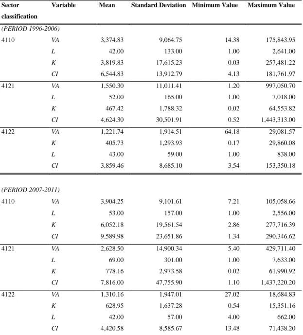
In order to control for the effect of the economic crisis, we estimate the model by dividing the sample period into two sub-periods: before the Housing Bubble Burst (1996-2006); and after the Housing Bubble Burst (2007-2011). Table 2 presents a summary statistics of the data in both periods.
Table 2: Summary statistics
Sector classification
Variable Mean Standard Deviation Minimum Value Maximum Value
(PERIOD 1996-2006) 4110 VA 3,374.83 9,064.75 14.38 175,843.95 L 42.00 133.00 1.00 2,641.00 K 3,819.83 17,615.23 0.03 257,481.22 CI 6,544.83 13,912.79 4.13 181,761.97 4121 VA 1,550.30 11,011.41 1.20 997,050.70 L 52.00 165.00 1.00 7,018.00 K 467.42 1,788.32 0.02 64,553.82 CI 4,624.30 30,501.91 0.52 1,443,313.00 4122 VA 1,221.74 1,914.51 64.18 29,081.57 K 405.73 1,293.93 0.17 29,860.08 L 43.00 59.00 1.00 838.00 CI 3,859.46 8,685.10 3.54 153,350.18 (PERIOD 2007-2011) 4110 VA 3,904.25 9,101.61 7.21 105,058.66 L 53.00 157.00 1.00 2,556.00 K 6,052.18 19,561.54 2.86 277,716.39 CI 9,589.98 23,651.86 1.34 290,346.62 4121 VA 2,628.50 14,900.34 5.40 429,711.40 L 69.00 301.00 1.00 7,633.00 K 778.16 2,973.58 0.02 61,990.92 CI 7,816.00 47,755.90 1.10 1,437,220.20 4122 VA 1,310.16 1,947.01 27.02 18,684.83 K 628.95 1,637.28 0.54 15,351.16 L 42.00 57.00 4.00 662.00 CI 4,420.58 8,585.67 13.48 71,438.20 Notes: Output (VA), capital (K) and Intermediate Comsumtions (IC) are in thousands of euros.
Variables VA, K and CI are deflated using the implicit deflator index of the construction GFCF. Prices used to deflate output and inputs are obtained from the Spanish Statistical Office (various years).
4.a. SFA Estimation
In order to estimate the production functions of each sector, from which obtain efficiency scores, we take as a starting point the translog specification (hereinafter translog).
The translog function is a more flexible extension of the Cobb-Douglas function therefore does not require a constant and unitary elasticity of substitution. Hence, the translog function can be seen as a combination of the Cobb-Douglas function and the quadratic function. To check whether the Cobb-Douglas production function is rejected in favor of the Translog production function, we will apply a likelihood ratio test.
The translog production function has following specification of the Stochastic frontier model (hereinafter SFA):
) ( ln ln ln ln ln ln ln 2 1 ln 2 1 ln 2 1 ln ln ln ln 2 2 1 3 2 23 3 1 13 2 1 12 2 3 33 2 2 22 2 1 11 3 3 2 2 1 1 0 it it it it it it it it it it it it it it it u v t t X X X X X X X X X X X X y (4.1) Where The subscript "i" denotes the ith sample firm i = 1, 2, ... N
The parameters k and kk with k = 1, 2, 3 are unknown parameters to be estimated.
The subscript "t" indicates the t-th year of the sample t = 1996,…2006 for period 1996-2006.
The variable lnyit denotes the output produced by each firm "i" and year "t".
Variables Xkit with k = 1,2,3 are the explanatory variables of the model per year
and per company.
v is a random error term assumed to be independently and identically distributed it
(iid) as N(0,V2).
u is a non-negative random variable which is assumed to account for technical it
inefficiency in production and are assumed to be iid as truncations at zero of the
N(,2)
There is also the variable t and t2which are a variables added here to measure the Hicks-neutral technical change.
In the estimation process, the estimation algorithm re-parameterizes the variance parameter of the noise term (V2) and the scale parameter of the inefficiency term (2) and
instead estimates the parameters 2=V2+2 and γ =2/(V2+2). The parameter γ lies
inefficiency term u is irrelevant and the results should be equal to OLS results. In contrast, if γ
is one, the noise term v is irrelevant and all deviations from the production frontier are
explained by technical inefficiency.
The coefficients 1, 2 and ₃ are the output elasticities of inputs, and the sum of them
gives us the elasticity of scale, which indicates the returns to scale.
For models are proposed as follows: Model 1.0 is the stochastic frontier production function in which the firm effects, u , have the time-varying structure defined in the last it
section; Model 1.1 is the case in which the u ’s have half-normal distribution, assumes that i = 0; Model 1.2 is the time-invariant model, assumes that = 0; Model 1.3 is the time-invariant
model in which the u ’s have half-normal distribution, assumes that i = = 0.
Table 3 displays the estimated coefficients for the period during the formation of the
Housing Bubble 1996-2006. Presented below the name of the sectors, in brackets, are the
names for the best model of each sector. To determine the most suitable model, we conducted various hypothesis test of restriction on the parameters of the production structure. the decision is made based on the generalized likelihood-ratio statistic (the t-test for the coefficient γ is not valid, because γ is bound to the interval [0, 1] and hence, cannot follow a t-distribution). These generalized likelihood ratio statistics along with the decision are reported in the Table 3.
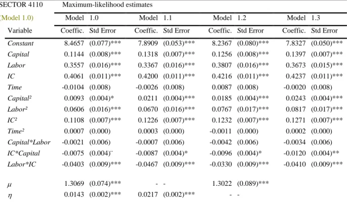
Table 3: Estimations and tests of hypothesis for three sectors (period 1996-2006 ) SECTOR 4110 Maximum-likelihood estimates
(Model 1.0) Model 1.0 Model 1.1 Model 1.2 Model 1.3
Variable Coeffic. Std Error Coeffic. Std Error Coeffic. Std Error Coeffic. Std Error Constant 8.4657 (0.077)*** 7.8909 (0.053)*** 8.2367 (0.080)*** 7.8327 (0.050)*** Capital 0.1144 (0.008)*** 0.1318 (0.007)*** 0.1256 (0.008)*** 0.1397 (0.007)*** Labor 0.3557 (0.016)*** 0.3367 (0.016)*** 0.3807 (0.016)*** 0.3673 (0.015)*** IC 0.4061 (0.011)*** 0.4200 (0.011)*** 0.4216 (0.011)*** 0.4237 (0.011)*** Time -0.0104 (0.008) -0.0026 (0.008) 0.0087 (0.008) -0.0020 (0.008) Capital² 0.0093 (0.004)* 0.0211 (0.004)*** 0.0185 (0.004)*** 0.0243 (0.004)*** Labor² 0.0606 (0.016)*** 0.0670 (0.016)*** 0.0767 (0.017)*** 0.0817 (0.017)*** IC² 0.1108 (0.007)*** 0.1226 (0.007)*** 0.1232 (0.007)*** 0.1271 (0.007)*** Time² 0.0007 (0.000) 0.0003 (0.000) -0.0011 (0.000) 0.0002 (0.000) Capital*Labor -0.0021 (0.006) -0.0007 (0.006) -0.0042 (0.006) -0.0034 (0.006) IC*Capital -0.0075 (0.004)¨ -0.0087 (0.004)* -0.0096 (0.004)* -0.0120 (0.004)** Labor*IC -0.0403 (0.009)*** -0.0467 (0.009)*** -0.0330 (0.009)*** -0.0410 (0.009)*** 1.3069 (0.074)*** - - 1.3022 (0.089)*** 0.0143 (0.002)*** 0.0217 (0.002)*** - -
2 =V 2 +2 0.6415 (0.027)*** 1.2891 (0.101)*** 0.6382 (0.039)*** 1.4440 (0.106)*** 0.6657 (0.011)*** 0.8224 (0.015)*** 0.6643 (0.014)*** 0.8370 (0.013)*** Log (likelihood) -3099.821 -3180.689 -3145.703 -3215.483
Test of hypothesis for parameters
Test Null hypothesis Assumptions 2
-statistics Decision TInv/SEff/Hnor m = = = 0 Model 1.0 3,981.5 *** Reject H0 T. Invar/H. normal = = 0 Model 1.0 449.9 *** Reject H0 Half Normal = 0 Model 1.0 411.8 *** Reject H0 Time Invariant = 0 Model 1.0 57.5 *** Reject H0 Stocastic Effect = 0 Model 1.0 1,824.0 *** Reject H0 Cobb Duglas β₆₋₁₂ = 0 Translog 268.9 *** Reject H0 Returns to
Scale
β₁₋₃ = 1 Decrising Returns to Scale 65.5 *** Reject H0
SECTOR 4121 Maximum-likelihood estimates
(Model 1.0) Model 1.0 Model 1.1 Model 1.2 Model 1.3
Variable Coeffic. Std Error Coeffic. Std Error Coeffic. Std Error Coeffic. Std Error Constant 7.2619 (0.013)*** 7.0298 (0.015)*** 7.2647 (0.013)*** 7.8327 (0.050)*** Capital 0.0824 (0.002)*** 0.0938 (0.002)*** 0.0818 (0.002)*** 0.1397 (0.007)*** Labor 0.4922 (0.006)*** 0.4951 (0.005)*** 0.4841 (0.006)*** 0.3673 (0.015)*** IC 0.2705 (0.003)*** 0.2702 (0.003)*** 0.2619 (0.003)*** 0.4237 (0.011)*** Time 0.0063 (0.002)** -0.0014 (0.002) 0.0070 (0.002)*** -0.0020 (0.008) Capital² 0.0316 (0.001)*** 0.0358 (0.001)*** 0.0330 (0.001)*** 0.0243 (0.004)*** Labor² 0.1877 (0.006)*** 0.2159 (0.005)*** 0.1789 (0.006)*** 0.0817 (0.017)*** IC² 0.1045 (0.003)*** 0.1050 (0.002)*** 0.0963 (0.002)*** 0.1271 (0.007)*** Time² -0.0007 (0.000)** 0.0002 (0.000) -0.0008 (0.000)*** 0.0002 (0.000) Capital*Labor -0.0074 (0.002)* -0.0116 (0.002)*** -0.0128 (0.002)*** -0.0034 (0.006) IC*Capital -0.0103 (0.001)*** -0.0094 (0.001)*** -0.0074 (0.001)*** -0.0120 (0.004)** Labor*IC -0.0878 (0.003)*** -0.0971 (0.003)*** -0.0779 (0.003)*** -0.0410 (0.009)*** 0.8556 (0.017)*** - - 0.8586 (0.018)*** - - -0.0033 (0.001)** -0.0040 (0.001)*** - - - - 2 =V 2 +2 0.2514 (0.006)*** 0.6520 (0.026)*** 0.2528 (0.007)*** 1.4440 (0.106)*** 0.7280 (0.004)*** 0.8843 (0.005)*** 0.7291 (0.004)*** 0.8370 (0.013)*** Log (likelihood) -5019.609 -5577.369 -5038.424 -5585.477
Test of hypothesis for parameters
Test Null hypothesis Assumptions 2
-statistics Decision TInv/SEff/Hnor m = = = 0 Model 1.0 13,598.0 *** Reject H0 T. Invar/H. normal = = 0 Model 1.0 1,131.7 *** Reject H0 Half Normal = 0 Model 1.0 1,115.5 *** Reject H0
Time Invariant = 0 Model 1.0 37.6 ** Reject H0 Stocastic
Effect
= 0 Model 1.0 9,852.6 *** Reject H0 Cobb Duglas β₆₋₁₂ = 0 Translog 3,170.4 *** Reject H0 Returns to
Scale
β₁₋₃ = 1 Decrising Returns to Scale 768.4 *** Reject H0
SECTOR 4122 Maximum-likelihood estimates
(Model 1.2) Model 1.0 Model 1.1 Model 1.2 Model 1.3
Variable Coeffic. Std Error Coeffic. Std Error Coeffic. Std Error Coeffic. Std Error Constant 7.0741 (0.047)*** 6.8925 (0.033)*** 7.0917 (0.062)*** 6.8868 (0.033)*** Capital 0.0906 (0.007)*** 0.1026 (0.007)*** 0.0900 (0.008)*** 0.1023 (0.007)*** Labor 0.4590 (0.016)*** 0.4640 (0.016)*** 0.4594 (0.015)*** 0.4687 (0.016)*** IC 0.2746 (0.010)*** 0.2701 (0.010)*** 0.2798 (0.010)*** 0.2732 (0.010)*** Time 0.0090 (0.006) 0.0035 (0.006) 0.0073 (0.006) 0.0037 (0.006) Capital² 0.0307 (0.004)*** 0.0339 (0.004)*** 0.0316 (0.005)*** 0.0341 (0.004)*** Labor² 0.2186 (0.020)*** 0.2351 (0.020)*** 0.2191 (0.020)*** 0.2374 (0.020)*** IC² 0.0884 (0.008)*** 0.0889 (0.008)*** 0.0907 (0.008)*** 0.0905 (0.008)*** Time² -0.0009 (0.000) -0.0004 (0.000) -0.0008 (0.000) -0.0004 (0.000) Capital*Labor -0.0543 (0.008)*** -0.0560 (0.008)*** -0.0536 (0.007)*** -0.0563 (0.007)*** IC*Capital 0.0054 (0.005) 0.0074 (0.005) 0.0026 (0.005) 0.0066 (0.005) Labor*IC -0.0431 (0.011)*** -0.0582 (0.011)*** -0.0422 (0.011)*** -0.0586 (0.011)*** 0.6135 (0.060)*** - - 0.6374 (0.076)*** - - 0.0034 (0.004) 0.0067 (0.004) - - - - 2 =V 2 +2 0.1547 (0.015)*** 0.3312 (0.034)*** 0.1637 (0.016)*** 0.3433 (0.034)*** 0.6084 (0.026)*** 0.8012 (0.022)*** 0.6204 (0.028)*** 0.8076 (0.021)*** Log (likelihood) -365.14 -387.01 -365.12 -388.27
Test of hypothesis for parameters
Test Null hypothesis Assumptions 2-statistics Decision
TInv/SEff/Hnor m = = = 0 Model 1.0 2,089.1 *** Reject H0 T. Invar/H. normal = = 0 Model 1.0 46.3 *** Reject H0 Half Normal = 0 Model 1.0 43.7 *** Reject H0
Time Invariant = 0 Model 1.0 0.04 Acept H0
Stocastic Effect
= 0 Model 1.2 () 847.8 *** Reject H0 Cobb Duglas β₆₋₁₂ = 0 Translog 330.5 *** Reject H0 Returns to
Scale
β₁₋₃ = 1 Decrising Returns to Scale 120.5 *** Reject H0
Signif. codes: 0 ‘***’, 0.01 ‘**’, 0.05 ‘*’, 0.10 ‘'’
The Cobb Douglas specification is rejected in all estimations in favor to the Translog specification. The null hypothesis, H0: = = = 0, is rejected in all the sectors. Therefore it
is evident that the average production function is not an adequate representation of the sample. Furthermore, the hypothesis that the half-normal distribution is an adequate representation for the distribution of the firm effects is also rejected (H0: = = 0 and H0: = 0). However, the
hypothesis that time-invariant model for firm effects is not rejected for the sectors 4122. Given that in this sector, the time-invariant is appropriated to define the firm effects.
Recapitulating, we select model 1.0 for the sectors 4110 and 4121, and the model 1.3 for the sector 4122.
The first order parameters in Table 3 can be identified as production elasticities evaluated at the sample means since all data were corrected by geometric mean before the estimation of SFA model. Looking in the elasticity of scale the results show that the sum of the parameters 1, 2 and ₃ are significantly different from one and, as a consequence, the sectors
present decreasing returns to scale with a parameter placed in the interval 0.88-0.83. Hence, if all firms increase all input quantities by one percent, the output quantity will usually increase by around 0.88-0.83 percent.
The coefficient of time (year of observation) is significant only for the sector 4121, and shows a slight technical progress in Hicks sense (average of 0.6 percent per year over the eleven-year period).
As the estimate of γ is 0.66 in sector 4110, 0.72 in sector 4121 and 0.62 in sector 4121, we conclude that both statistical noise and inefficiency are important for explaining deviations from the production function but that inefficiency is more important than noise. As 2 is not equal to the variance of the inefficiency termu, the estimated parameter γ cannot be interpreted as the proportion of the total variance that is due to inefficiency.
As neither the noise term v nor the inefficiency term it u but only the total error term it = vit uit is known, the technical efficiencies =
are generally unknown.
However, given that the parameter estimates (including the parameters 2 and γ or V2and 2)
and the total error term are known, it is possible to determine the expected value of the
technical efficiency (Coelli et al., 2005):
̂ [ ] (4.2)
We repeat the same estimation process for the sample of the period during de Financial Crisis 2007-2011. Table 4 provides the information about the Technical Efficiency before
(1996-2006) and after (2007-2011) the Housing Bubble Burst (Hereinafter HBB). Information about size sample and Returns to Scale are also shown.
Table 4: Technical Efficiency period 1996-2006 and 2007-2011 Period of
time
SECTOR 4110 SECTOR 4121 SECTOR 4122
N T.E. Returns to Scale N T.E. Returns to Scale N T.E. Returns to Scale 1996-2006 3,804 0.27 0.88 19,845 0.43 0.85 2,040 0.55 0.83 2007-2011 1,026 0.33 0.86 6,360 0.75 0.99 701 0.77 0.97
In the same way as show in Table 4, the graphs shows in Figure 2 presents the Kernel density estimates of Technical Efficiency for time-period before and after the beginning of the financial crisis (from 1996 to 2006, and from 2007 to 2011) for each sector.
Sector 4110 “Real estate development” shows the smallest mean efficiency in both periods, as well as a smaller difference between the two periods. Sector 4121” Residential buildings construction” in the in the opposite case is the sector with the greatest increase in TE contrasting the period before the financial crisis (0.43) to the period during the financial crisis (0.75). A possible first interpretation can be derived from this result: some technical inefficient firms might have been forced to disappear from the market due to the decrease in demand caused by the crisis. However, we can assure looking to the returns of scale that the increases in the average scale efficiency between periods as a result of the exit of scale inefficient firms. Figure 2. Kernel density estimates for Technical Efficiency pre- and post- Housing Bubble Burst
Sector 4121. Technical Efficiency (Kernel Density)
Further insights can be achieved by splitting the sample of efficiency estimates into construction firms that are active versus those that exit the sector due to bankruptcy. To compare the efficiency of Spanish construction firms operating in Housing Bubble formation period 1996-2006, we separate the sample into two subsamples: bankrupt companies in the period 2007-2011 and active companies in the period 2007-2011. Table 4 presents the figures and Figure 3 presents the Kernel density estimates of TE of these two categories of firms’ situation for the period from 1996 to 2006.
Table 4: Technical Efficiency period 1996-2006
Companies SECTOR 4110 SECTOR 4121 SECTOR 4122
N T.E. N T.E. N T.E.
Backrupt in period 2007-2011 937 0.34 4,143 0.40 605 0.49 Actives in period 2007-2011 2,867 0.27 15,702 0.45 1,435 0.57
Whit the exception of sector 4110 Figure 3 suggests that TE is slightly lower for construction firms that went bankrupt than for active firms. Thereby, we can confirm for sectors 4121 and 4122 that in average, some technical inefficient firms have been forced to disappear from the market in the period 2007-2011.
Figure 3. Kernel density estimates for Technical Efficiency period 1996-2006
Sector 4121. Technical Efficiency (Kernel Density)
4.b. Factors Affecting Efficiency
A number of hypothesis were investigated with the intention of assess the relative influence of these explanatory factors and others random effects. As explained above, we will use the Technical Inefficiency Effects model (TIE) Battese and Coelli (1995). With the assumptions developed in section 3 in place, the parametric mean of the density function, , can be defined as
(4.3)
We include the Year variable in the Technical Inefficiency Effects model to account for the changes in the technical inefficiency as time increases. We should clarify that this inclusion is compatible with Year variable include in the Stochastic Frontier Model, accounting for possible Hicks-Neutral technological change (Coelli and Battese, 1996). The technical inefficiency effects model discussed in section 3 is only useful when the inefficiency effects are stochastic and follow a specific distribution.
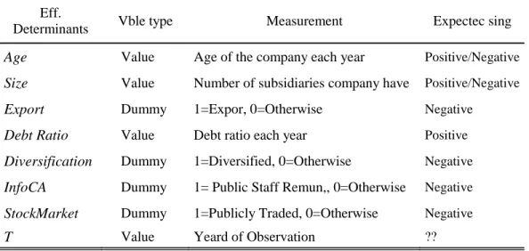
The definition and expected signs of the explanatory variables used in this study are presented in Table 5.
Table 5: List of explanatory variables
Eff.
Determinants Vble type Measurement Expectec sing
Age Value Age of the company each year Positive/Negative
Size Value Number of subsidiaries company have Positive/Negative
Export Dummy 1=Expor, 0=Otherwise Negative
Debt Ratio Value Debt ratio each year Positive
Diversification Dummy 1=Diversified, 0=Otherwise Negative
InfoCA Dummy 1= Public Staff Remun,, 0=Otherwise Negative
StockMarket Dummy 1=Publicly Traded, 0=Otherwise Negative
T Value Yeard of Observation ??
The expected sign of the δ-parameters in the inefficiency model are not clear in all cases. The Older firms could be expected to have more experience and hence have less inefficiency. However Older firms are also likely to be more accommodate and thereby perhaps more inefficient.
During the period post- HBB (2007-2011) the Spanish construction industry has undergone a hardship due to the excessive usage of debt. As You and Zi (2007) argued, there are some conflicting theories on the relationship between corporate leverage and efficiency. Spanish construction firms had been excessively levered and suffered from severe cash flow shortage. Therefore, we expect that the negative effect of leverage dominates the positive effect and high leverage ratio influences positively inefficiency.
Export and Diversification may be viewed as a market strategy. Economists suggest the
reinsurance effect hypothesis that a firm’s diversification reduces its profit variability through a business portfolio effect and thus increases its value (Lewellen, 1971).
InfoAC and StockMarket are variables related to corporate transparency. Listed
companies are required to make additional retirement of information. Shareholders will have a better understanding of the real situation of the company and will act accordingly. For this reason, we consider that to be a listed company should be associated with less technical inefficiency. We use the same argument of transparency for companies that report board of directors’ remuneration.
We estimate the Technical Inefficiency Effects Model with all sectors included for both periods, pre- HBB (1996-2006) and post-HBB (2007-2011). The results are shown in Table 6.
All coefficients in the TIE Model are significant (at 1% significance level), and null hypothesis about joint significance of the variables were both rejected at the one percent level of significance which proves that variables are jointly significant.
We look at the sense of the signs because the size of the coefficients of the TIE model (δ) cannot be reasonably interpreted1
. In the manner we expected Info AC and StockMarket are significantly negative, which means that corporate transparent firms are significantly more technical efficient. Age is significantly negative, which means that older firms are significantly more efficient and Year is significantly positive, which means that as time increases technical inefficiency increase.
Export and Debt Ratio behaves as the expected sense in the post HBB period
(2007-2011), but opposite as expected in the pre-crisis period. Intuitively we might think that, for the
Export variable, during the formation of the housing bubble, domestic market generate greater
returns to investment than foreign market and after housing bubble burst, foreign market becomes more attractive. Debt Ratio behaviors could be associated with the patterns on
1 Marginal effects of the variables that should explain the efficiency level on the efficiency estimates can be calculate following Olsen and Henningsen, (2011).
financial system and the lack of liquidity after the HBB. Spanish firms with high leverage ratio and involved in liquidity and credit problems are adversely affected in their technical efficiency level.
Table 6: Technical Efficiency Effects Frontier for period 1996-2006 and period 2007-2011
Pre- HBB (1996-2006) Post- HBB (2007-2011)
Variable Coefficient Std Error Expected Variable Coefficient Std Error Expected
Constant -1635.0687 255.9*** Constant -8977.6941 1862.***
Age -2.2019 0.317***
√
Age -1.0417 0.224***√
Size 337.8483 52.23***
√
Size 686.0974 143.0***√
Export 254.8382 39.39***
X
Export -100.2490 20.93***√
Debt Ratio -1.0622 0.157***
X
Debt Ratio 0.0585 0.021**√
Diversification 98.8224 15.37***
X
Diversification -58.6194 12.24***√
InfoAC -170.1813 27.07***√
InfoAC -115.5026 24.23***√
StockMarket -816.4395 126.2***√
StockMarket -11.6104 1.166***√
Year 14.8569 2.324*** Year 413.2766 85.65*** 2 =V 2 +2 218.4176 34.18*** 2=V 2 +2 696.1464 144.4*** 0.9992 0.000*** 0.9998 0.000***Test of hypothesis for parameters Test of hypothesis for parameters
Test Null hypothesis -statist. Decision Test Null hypothesis -statist. Decision Efficiency effects = δ₁₋₈ = 0 179.1*** Reject H0 Efficiency effects = δ₁₋₈ = 0 99.1*** Reject H0 Joint effects of
Ineff. Determinants
δ₁₋₈= 0 162.9*** Reject H0 Joint effects of Ineff. Determinants δ₁₋₈= 0 84.9*** Reject H0 Signif. codes: 0 ‘***’, 0.01 ‘**’, 0.05 ‘*’, 0.10 ‘'’ 5. Concluding comments.
The Spanish construction sector enjoyed a period of constant growth and played an important role in the development of the Spanish economy over the past several decades. However, the burst of the Spanish Housing Bubble in 2007 had made the construction sector undergo unprecedented hardships. A drastic decrease in demand for new housing added to the high external debt that the companies suffer from cause the wholesale collapse of its industry generating that from 2007 to 2013 one in two building companies has closed.
This is the first empirical study examines the technical efficiency of Spanish Construction sector using Stochastic Frontier Analysis Model. This study estimates technical
efficiency of the firms under the three sectors related to Spanish building activity before and after the Housing Bubble Burst and compares the firms that went bankrupt versus those that were not. The empirical application used accountancy data from 2,815 construction firms in the period 1996-2011. We also identify several important factors of the efficiency change.
In all sectors, Technical Efficiency is significantly larger after the beginning of the financial crisis than before the financial crisis. The improvement is mainly due to the disappearance of large number of companies on average, more Technical Inefficient. Increases in the average scale efficiency between periods were founds for two sectors as a result of the exit of scale inefficient firms during the financial crisis.
Meanwhile, the results from the SFA method shows that Age affects positively the technical efficiency and corporate transparency firms have high levels of Technical Efficiency.
Export and the leverage ratio variation are also significantly related with the TE level.
But, this variables sign varies with the period we consider, pre-crisis or during-crisis. This behavior confirms the hypothesis suggesting that construction industry is an activity cyclically sensitive. At this point politics suggestions may arise, counter-cyclical policies to preserve economic and financial stability should be expanded in the sector. Promoting financial assistance to the companies in times of economic crisis and promoting export and diversification of the companies in expansive economic cycle could be measures consistent with this study.
Finally, the SFA method was used in this study, however, alternative ways to estimate technical efficiency while incorporating explanatory variables do exist. For example, DEA estimation methods could be considered in future work, to investigate the influence of methodology choice upon our empirical results.
References
AIGNER, D., LOVELL, C.A.K. and SCHMIDT, P., 1977. Formulation and estimation of stochastic frontier production function models. Journal of Econometrics, 6(1), pp. 21-37.
BANKER, R.D., CHARNES, A. and COOPER, W.W., 1984. SOME MODELS FOR ESTIMATING TECHNICAL AND SCALE INEFFICIENCIES IN DATA ENVELOPMENT ANALYSIS.
Management Science, 30(9), pp. 1078-1092.
BATTESE, G.E. and COELLI, T.J., 1995. A model for technical inefficiency effects in a stochastic frontier production function for panel data. Empirical Economics, 20(2), pp. 325-332.
BATTESE, G.E. and COELLI, T.J., 1992. Frontier production functions, technical efficiency and panel data: With application to paddy farmers in India. Journal of Productivity Analysis, 3(1-2), pp. 153-169. BATTESE, G. and G. CORRA, 1977. Estimation of a Production Frontier Model: With Application to the Pastoral Zone of Eastern Australia. Australian Journal of Agricultural Economics, 21(1), pp. 167 179.
CHARNES, A., COOPER, W.W. and RHODES, E., 1978. Measuring the efficiency of decision making units. European Journal of Operational Research, 2(6), pp. 429-444.
COELLI, T. and BATTESE, G., 1996. Identification of factors which influence the technical
inefficiency of Indian farmers. Australian Journal of Agricultural and Resource Economics, 40(2), pp. 103-128.
COELLI, T., 2005. An introduction to efficiency and productivity analysis. Springer Science+Business Media, cop. 2005.
COTO-MILLÁN, P., BAÑOS-PINO, J. and RODRÍGUEZ-ÁLVAREZ, A., 2000. Economic efficiency in Spanish ports: Some empirical evidence. Maritime Policy and Management, 27(2), pp. 169-174. COTO-MILLAN, P., INGLADA, V. and REY, B., RODRÍGUEZ-ALVAREZ, A., 2006. Liberalisation and efficiency in international air transport. Transportation Research Part A: Policy and Practice, 40(2), pp. 95-105.
DZENG, R.-. and WU, J.-., 2013. Efficiency measurement of the construction industry in Taiwan: a stochastic frontier cost function approach. Construction Management and Economics, 31(4), pp. 335-344.
EL-MASHALEH, M.S., RABABEH, S.M. and HYARI, K.H., 2010. Utilizing data envelopment analysis to benchmark safety performance of construction contractors. International Journal of Project
Management, 28(1), pp. 61-67.
FARRELL, M.J., 1957. The Measurement of Productive Efficiency. Journal of the Royal Statistical
Society.Series A (General), 120(3), pp. 253-290.
FERNÁNDEZ, C., KOOP, G. and STEEL, M., 2000. A Bayesian analysis of multiple-output production frontiers. Journal of Econometrics, 98(1), pp. 47-79.
GREENE, W., 2005. Fixed and random effects in stochastic frontier models. Journal of Productivity
Analysis, 23(1), pp. 7-32.
GREENE, W., 2005. Reconsidering heterogeneity in panel data estimators of the stochastic frontier model. Journal of Econometrics, 126(2), pp. 269-303.
GREENE, W., 2000. LIMDEP computer program: Econometric Software, Plainview, New York. GREENE, W.H., 1980. Maximum likelihood estimation of econometric frontier functions. Journal of
Econometrics, 13(1), pp. 27-56.
HORTA, I.M. and CAMANHO, A.S., 2013. Company failure prediction in the construction industry.
Expert Systems with Applications, 40(16), pp. 6253-6257.
HORTA, I.M., CAMANHO, A.S., JOHNES, J. and JOHNES, G., 2013. Performance trends in the construction industry worldwide: An overview of the turn of the century. Journal of Productivity
Analysis, 39(1), pp. 89-99.
KUOSMANEN, T., 2012. Stochastic semi-nonparametric frontier estimation of electricity distribution networks: Application of the StoNED method in the Finnish regulatory model. Energy Economics, 34(6), pp. 2189-2199.
LEE, L., 1993. Asymptotic Distribution of the Maximum Likelihood Estimator for a Stochastic Frontier Function Model with a Singular Information Matrix. Econometric Theory, 9(3), pp. 413-430.
LEE, Y., and SCHMIDT, P., 1993. A Production Frontier Model with Flexible Temporal Variation in Technical Efficiency. in H. Fried, K. Lovell and S. Schmidt. The Measurement of Productive
Efficiency, Oxford University Press, Oxford.
LEWELLEN, W.,1971. A Pure Financial Rationale for the Conglomerate Merger. Journal of Finance.
American Finance Association, 26(2), pp. 521-37.
MOSCARINI, G. and POSTEL-VINAY, F., 2008. The timing of labor market expansions: New facts
and a new hypothesis.
OLSEN, J.V., and HENNINGSEN, A., 2011. Investment Utilization and Farm Efficiency in Danish Agriculture. Institute of Food and Resource Economics, FOI Working Paper No. 2011/13.
OREA, L. and KUMBHAKAR, S.C., 2004. Efficiency measurement using a latent class stochastic frontier model. Empirical Economics, 29(1), pp. 169-183.
PILATERIS, P. and MCCABE, B., 2003. Contractor financial evaluation model (CFEM). Canadian
Journal of Civil Engineering, 30(3), pp. 487-499.
PITT, M.M. and LEE, L.-., 1981. The measurement and sources of technical inefficiency in the Indonesian weaving industry. Journal of Development Economics, 9(1), pp. 43-64.
RUGGIERO, J., 2004. Performance evaluation when non-discretionary factors correlate with technical efficiency. European Journal of Operational Research, 159(1), pp. 250-257.
RUGGIERO, J., 2007. A comparison of DEA and the stochastic frontier model using panel data.
International Transactions in Operational Research, 14(3), pp. 259-266.
SEE, K.F. and COELLI, T., 2012. An analysis of factors that influence the technical efficiency of Malaysian thermal power plants. Energy Economics, 34(3), pp. 677-685.
SHEPHARD, R., 1953, Cost and Production Functions. Princeton University Press, Princeton. SIMAR, L. and ZELENYUK, V., 2011. Stochastic FDH/DEA estimators for frontier analysis. Journal
of Productivity Analysis, 36(1), pp. 1-20.
STEVENSON, R.E., 1980. Likelihood functions for generalized stochastic frontier estimation. Journal
of Econometrics, 13(1), pp. 57-66.
TAEWOO YOU and HONGMIN ZI, 2007. The economic crisis and efficiency change: evidence from the Korean construction industry. Applied Economics, 39(14), pp. 1833-1842.
TSOLAS, I.E., 2011. Modelling profitability and effectiveness of Greek-listed construction firms: An integrated DEA and ratio analysis. Construction Management and Economics, 29(8), pp. 795-807. WANG, H.-. and SCHMIDT, P., 2002. One-step and two-step estimation of the effects of exogenous variables on technical efficiency levels. Journal of Productivity Analysis, 18(2), pp. 129-144. YOU, T. and ZI, H., 2007. The economic crisis and efficiency change: Evidence from the Korean construction industry. Applied Economics, 39(14), pp. 1833-1842.