Grading latin american presidents : a view from the stock markets

Texto completo

(1)Cruces, Juan José ; García-Cicco, Javier. Grading latin american presidents : a view from the stock markets. Documento de Trabajo Nº 37 Facultad de Ciencias Económicas Escuela de Economía “Francisco Valsecchi”. Este documento está disponible en la Biblioteca Digital de la Universidad Católica Argentina, repositorio institucional desarrollado por la Biblioteca Central “San Benito Abad”. Su objetivo es difundir y preservar la producción intelectual de la Institución. La Biblioteca posee la autorización del autor para su divulgación en línea.. Cómo citar el documento: Cruces, J.J., García-Cicco, J. (2012, junio). Grading latin american presidents : a view from the stock markets [en línea]. Documento de trabajo No. 37. Escuela de Economía “Francisco Valsecchi”. Facultad de Economía de la Universidad Católica Argentina. Disponible en: http://bibliotecadigital.uca.edu.ar/repositorio/investigacion/gradinglatin-american-presidents.pdf (Se recomienda indicar fecha de consulta al final de la cita. Ej: [Fecha de consulta: 19 de agosto de 2010])..

(2) DOCUMENTOS DE TRABAJO. Pontificia Universidad Católica Argentina “Santa María de los Buenos Aires”. Grading Latin American Presidents: A View from the Stock Markets. Por Juan José Cruces y Javier García-Cicco. Facultad de Ciencias Económicas Escuela de Economía “Francisco Valsecchi” Documento de Trabajo Nº 37 Junio de 2012.

(3) Los autores del presente artículo ceden sus derechos, en forma no exclusiva, para que se incorpore la versión digital del mismo al Repositorio Institucional de la Universidad Católica Argentina y a otras bases de datos que la Universidad considere de relevancia académica..

(4) Preliminary, comments welcome. Grading Latin American Presidents: A View from the Stock Markets* Juan José Cruces. †. Universidad Torcuato Di Tella. ‡. Javier García-Cicco. Universidad Católica Argentina Central Bank of Chile June 2012 Abstract. We use stock returns to grade presidential economic performance. In efficient markets, asset prices are unique in that they impound the long term effects of changes in the environment, including government policy. To purge national returns of state-of-the-world conditions that do not result from local events, we introduce a global twin portfolio and a regional return. The twin portfolio for a country reports the return of a combination of world stocks that each month has the same industrial composition as that one country’s stock index. These benchmark external conditions are most volatile: they vary between a 295% appreciation (or tailwind under some interpretations) and a 30% reduction (or headwind) in asset prices over extreme four-year presidencies in our sample. We interpret the gap of national performance over these counterfactual returns as a proxy for the quality of domestic policies during a given presidency, as seen from the standpoint of equity investors. We apply this approach to seven Latin American countries from 1980 until 2011. From this perspective, Colombia, Peru and Chile stand out as the countries that have implemented the best long run policies over the sample. In addition, we provide a grading of relative presidential performance. JEL Codes: G15, G14, H11, E44 Keywords: Benchmarking presidential performance, Measuring global tailwind, Latin America. *. We would like to thank José Luis Machinea, Paul Malatesta, Juan Pablo Nicolini, Guido Sandleris and Gustavo Reist for comments, Alejandro Izquierdo for providing quarterly terms of trade data and Urbi Garay for providing Venezuelan market exchange rate data. Special thanks go to Roby Muntoni and Michael Orzano from S&P Index Services. Isaac Fainstein, Pablo González Ginestet and Matías Vieyra provided excellent research assistance. The views and conclusions presented in this paper are exclusively those of the authors and do not necessarily reflect the position of the Central Bank of Chile or its Board members. † Business School, Sáenz Valiente 1010, C1428BIJ – Buenos Aires, Argentina. Ph.: +54-11-5169-7301, Fax: +54-11-5169-7347. Email: [email protected]. ‡ Economics Department, A. M. de Justo 1300, C1107AAZ – Buenos Aires, Argentina. Ph.: +54-11-43490200. Email: [email protected], [email protected]..

(5) “I hold it to be true that Fortune is the arbiter of one-half of our actions, but that she still leaves us to direct the other half, or perhaps a little less.” Niccoló Machiavelli, The Prince (1515). 1. Introduction The last decade has been particularly prosperous throughout Latin America, especially when compared to the previous 20 years. The average annual real GDP growth and the average annual real stock price increase for the seven largest countries were much larger from 2001 until 2010 than from 1981 until 2000.1 It is noteworthy that this remarkable improvement has been accompanied by starkly contrasting economic policy approaches in the cross section: some countries have sought trade openness while others have curtailed both imports and exports; some countries have had inflation below 5% and others above 20%; some countries have courted foreign investors while others have shunned them away2; some have built-up assets (oil and gas reserves, heads of livestock, social security and sovereign wealth funds, etc.) while others have depleted them. While each government claims that the contemporaneous success speaks to the suitability of their own policies, it cannot be the case that all of them are right unless country conditions are so specific that they require policies that are almost opposite to one another. An alternative hypothesis is that the recent wellbeing may result from a favorable aggregate shock that affects the region as a whole, making the effects of local policies of second order importance. The purpose of this paper is to present a methodology to establish a fair benchmark against which economic outcomes during a given presidential term can be compared. This requires overcoming two hurdles: choosing a measure of performance and building a counterfactual. Our methodology is based on publicly listed stock prices. Presidents in office often blame their predecessors for current misfortunes and claim to be making the right decisions for the long run. In efficient markets, both of these circumstances would be reflected in asset prices, giving current presidents an amount of credit for their actions that is not systematically biased and that takes into account the perceived long-run effects of their policies. Other variables that are relatively more backward looking (notably GDP) may underestimate the intertemporal effects often inherent in economic policy. In other words, our approach will be gauging the quality of policy by the perceived value generated to equity owners at the time that the market learns of them. The methodology consists of decomposing the monthly return of the national stock market index in a global, a regional, and a national differential component. The counterfactual return is the sum of the global plus the regional component. 1. The average annual figures were, respectively, 3.7% and 16.9% during 2001-2010 compared to 2.5% and 8.7% during 1981-2000. The sample includes Argentina, Brazil, Colombia, Chile, Mexico, Peru and Venezuela. Stock figures are from the S&P/IFC national indices and GDP figures are from the World Bank and expressed in PPP dollars. 2 “Mr. President: You have insulted us all,” said the president of the Spanish Confederation of Employers' Organizations, the major representative institution of the Spanish business community to Argentina’s Néstor Kirchner in 2003, (http://www.elmundo.es/elmundo/2003/07/17/espana/1058450089.html). Spain was the major source of foreign direct investment in Argentina during the 1990s.. 1.

(6) Correctly identifying a global benchmark return is most important. For example, during 2011, the S&P500 stock market index fell 3%, while the S&P/IFC Mexican index fell 9% and the Peruvian index fell 30%, all in local inflation-adjusted units. A naïve interpretation of these figures would indicate substantial underperformance of the two latter countries. However, the industrial structures of the three indices are very different because the latter countries have much less diversified economies. Our key methodological innovation is to construct a global twin index for each country which uses industry portfolio returns from the whole world but that, each month, has the same industrial composition as the country in question. The global twin index for Mexico fell 13% during 2011 while that for Peru fell 38%. So holding industrial composition constant, the two countries actually did much better than their world counterparts, contrary to what seems at first. Furthermore, it is possible that Latin America performed better on average than the twin indices due to a regional shock (such as a change in investor risk appetite, capital flow swings, climate shocks like the El Niño, or shocks to regional terms of trade) and a fair benchmarking of presidential performance over time should also account for this factor. In fact, our results indicate that high returns and low volatility of this factor are the hallmarks that distinguish the last decade from the previous 20 years. The data show that it is critical to account for the worldwide bonanza of different time periods. The summary external conditions reflected in the counterfactual returns varied between a 295% appreciation and a 30% reduction in asset prices over extreme four-year presidencies in our sample. So some presidents faced a period of significant global windfall while others were met by dire straits. We interpret the national differential return over this benchmark during a large sample as reflecting a host of country-specific conditions that include the quality of economic policy announced during this time from the viewpoint of equity investors. We use the mean national differential return during its tenure in office as the grade that each president obtains on our scale. We apply our approach to Argentina, Brazil, Chile, Colombia, Mexico, Peru, and Venezuela from 1980 until 2011. We document three key empirical findings. First, the regional factor which contributed an average annual return of 1.9% during 1980-2001 contributed an annual return of 8.8% during 2002-2011. Moreover, this component has been remarkably stable over the recent period compared to the earlier one: it explained about one-third of the total volatility of returns during 1980-2001 while it only explained about one-twentieth of that volatility during 2002-2011.3 There is no doubt that the region experienced an unusually long period of stable bonanza during the last decade. Second, Colombia, Peru and Chile have been the countries in the sample with the largest gains relative to the benchmark. The gaps in differential performance are very significant: the control portfolio for Colombia during its 27 years in the sample rose from 1 to 41 3. The standard deviation of annual returns also fell over time: it was 49% in the early period while it was 33% in the more recent one.. 2.

(7) consumption units, while the Colombian stock index rose from 1 to 120 consumption units, almost tripling the benchmark returns. Peru’s control portfolio rose from 1 to 8.5 consumption units but the Peruvian index rose from 1 to 18.5 during its 19 years in the sample. Chile was in the sample during 32 years, which included the early 1980s debt crisis, so it had lower own and benchmark performance. Overall, its benchmark world portfolio appreciated from 1 to 24 consumption units, while Chile rose from 1 to 38. At the other end, during its 19 years in the sample, the control portfolio for Venezuela rose from 1 to 4.2 consumption units, but the Venezuelan index rose from 1 to 1.3 consumption units. Last, the best performing presidents in the sample were Franco and Figueiredo (Brazil), Barco, Gaviria and Uribe’s first term (Colombia) whose national differential returns exceeded 15% per year. The worst performers were López Portillo (Mexico), Bentacur and Samper (Colombia), Sarney (Brazil), De la Rúa, Alfonsín and Cristina Fernández de Kirchner (Argentina) during whose tenure the national differential contributions were below -14% per year.. 1.1.. Related Literature. Our work is related to two different strands of the literature. On the one hand, a number of papers analyze the impact of particular policy announcements on the stock market. For instance, Henry (2000) looks at the impact of stock market liberalization policies, Andritzky et al. (2007) study the impact of macroeconomic news on bond prices in emerging countries, while Arslanalp and Henry (2005) analyze the stock market impact of debt relief agreements under the Brady plan. More recently, Raddatz (2011) studies the impact of multilateral debt relief announcements on the stock prices of South African companies with subsidiaries in countries benefited by these initiatives, while Moser and Rose (2011) analyze the impact of regional-trade-agreements announcements on stock market indices. All of these studies share a methodological approach, namely the estimation of abnormal returns associated with specific policy measures. By contrast, we characterize not the effect of a narrowly defined policy announcement but the overall effect of policies and economic management during a given presidential period. We do this by comparing the performance of the national index during such a period to that of a counterfactual portfolio. The counterfactual attempts to capture the return of a portfolio of stocks that satisfy two conditions: a) they represent the same industries as those listed in the country’s market but they are immune from local policies, and b) they are similarly exposed to the average Latin American regional shocks. On the other hand, this paper is also related to the literature assessing the relative role of local policies and external shocks in determining the economic performance. One of the seminal papers in this literature is the work by Easterly et al. (1993) which documents that fluctuations in terms of trade are more important in explaining the variance of GDP growth than changes in institutions. According to the authors’ interpretation, good policy (i.e. institutional change) cannot be the main source of long-run growth, while good luck appears as a better explanation. Many studies have followed this work, trying to disentangle the relative role of good luck in explaining GDP fluctuations. Some examples are Easterly et al. (1997), della Paolera et al. (2003), and Cecchetti et al. (2011). Another prolific 3.

(8) literature analyzes the role of external factors in explaining macroeconomic fluctuations in emerging countries. Some of these papers use vector auto-regression models, like Hoffmaister and Roldos (1997), Izquierdo et al. (2008), Österholm and Zettelmeyer (2008), Boschi and Girardi (2011) and Aiolfi et al. (2011). Another group of papers uses dynamic stochastic general equilibrium (DSGE) models. For instance, Neumeyer and Perri (2005) and Uribe and Yue (2006) analyze the importance of world interest rate shocks and country premium for emerging countries; while Mendoza (1995) focuses on the importance of terms of trade shocks. A somewhat different but related paper is Levy-Yeyati and Cohan (2011) which reports a global wind index that synthesizes the role of external factors in explaining GDP growth in the seven largest Latin American countries. Our global plus regional contribution can also be interpreted (with some caveats discussed below) as a global wind index and we compare the results of both approaches below. Although there are many methodological differences among these studies, and between them and our paper, the main conceptual difference is our focus on asset prices instead of macroeconomic aggregates which, as we argue, allow to better capture the intertemporal effects of domestic policies. Nonetheless, it is worth emphasizing that although our paper has some links to these previous studies, to the best of our knowledge we are the first to propose a methodology to grade the economic performance during different presidential periods using information from the stock market. The rest of the paper is organized as follows. Section 2 discusses the benefits and limitations of relying on stock market prices to assess the quality of policies and lays down a simple conceptual framework to understand how different factors may affect the national stock index. Section 3 describes the data and defines the variables of interest. Section 4 presents the econometric methodology and discusses the results, including several robustness exercises. Section 5 concludes.. 2. Conceptual framework In this section we first discuss the benefits and drawbacks of using stock prices to assess the quality of economic policy. We then present a simple conceptual framework to understand how stock prices are affected by national, regional and global conditions.. 2.1.. The pros and cons of stock prices to assess the quality of policy. In assessing the impact of government policies, the ideal object of study would be the contribution of each administration to the present value of the stream of income to the owners of human and physical capital. The general choice in the literature is some macroeconomic aggregate, generally the growth rate of real GDP, which is the current value of income. If there were no business cycles and if the short run effects of policies were equal to their long run effects, this would be just fine as the present value is a simple monotonic function of this rate. But unfortunately this is not the case. Given that the present value of future labor income is not priced in a market, we focus on the price of the future value of corporate profits for which there is a market. We analyze the broadest observable measure which is the value of a diversified (capitalization-weighted) basket of 4.

(9) publicly listed local equities, acknowledging upfront that not all equity claims in an economy trade in publicly listed markets. Specifically, we assess the change in the value of this basket, measured in local units of consumption, over the whole sample or over the term of a given presidency. Thus, we will be grading presidential administrations from the standpoint of a local buy-and-hold investor. We next analyze the advantages and disadvantages of our metric relative to the common practice in related literatures. Using GDP growth to assess the impact of economic policy has several drawbacks. First, economic policy typically involves important intertemporal effects as policies that are implemented by one president may have their full effects during the tenure of her successors. For instance, one administration may implement policies that spur growth immediately, but which are detrimental to long term growth (e.g. by depleting the stock of a non-renewable resource, like minerals, or a renewable one, like international reputation). The reverse often takes place as well, as the discovery or entering into operation of new capital stock may raise GDP today although it is the result of long-held policies of predecessors (e.g. the natural gas pipeline from Camisea to Lima in Peru, or the discovery of new oil fields in Brazil’s Atlantic shore). Another example is countercyclical policy; for instance, fiscal rules to save the proceedings from temporary increases in commodity exports. While such policies are generally considered desirable from a long run perspective, a country that runs a countercyclical policy in a booming period will likely experience, ceteris paribus, a smaller increase in GDP than another one that does not.4 These examples highlight the fact that GDP is to a large extent a backward-looking variable, and therefore can give a wrong measure of the quality of policy during a given presidency. By contrast, in efficient markets, the price of assets will rapidly reflect the perceived short- and the long-term effects of policy at the time that the market learns of it. Moreover, using stock prices simplifies controlling for changes in external conditions and for business cycle effects in order to identify idiosyncratic shocks. However, the proposed measure has some drawbacks as well. First, to the extent that there may be distributional effects between providers of labor and owners of capital within a country, it should be emphasized that when we refer to the effects of policy, we mean from the point of view of equity investors. Moreover, there could be distributional effects between equity- and debt-holders. For example, when Argentina amended the law to avoid generalized bankruptcies in the 2002 crisis, it transferred wealth from debt holders to equity holders and this will increase the grade of the president in office on our metric. Last, there could be distributional effects within the corporate sector, either in favor or against the listed corporations. For example, a government that has a pro-small business approach will 4. Using GDP growth has other problems that can be partly overcome using econometric techniques (this is the case, for instance, in most of the VAR based literature): a) business cycles fluctuations: governments taking office at the trough of the cycle are likely to witness a GDP increase regardless of the policy that they implement, b) interdependence: sorting out a country’s idiosyncratic growth from that induced by world or regional growth, c) terms of trade effects: positive shocks to terms of trade can induce several effects in real growth through different channels (e.g. import of production factors) unrelated to government policy.. 5.

(10) be creating more shareholder value than our measure might acknowledge, given that it is large firms that are publicly listed. Second, financial markets are not as deep in Latin America as in developed economies, a fact that has two consequences. First, publicly-listed firms generally represent a small percentage of the total value of the capital stock in the economy. However, it is noteworthy that private equity transactions often take valuation multiples from publicly listed equities in the local market. Hence, while this is a limitation, it is not obvious that it should bias the results. Second, with the possible exception of Brazil and Mexico, these markets are often illiquid by international standards, which could cause informationally inefficient pricing. This would be problematic if we were doing intraday analysis, but seems less important for an exercise like ours that is based on month-end prices over 32 years.5 Third, Latin American governments have many times imposed restrictions on international capital movements. On the one hand, such restrictions will decrease the value of stocks because the foreign demand for domestic stocks is restricted. But on the other hand, during some episodes of severe capital controls, the stock market has served as a device to take money out of the country (see, e.g. Auguste et al., 2006, among others), actually rising stock prices. Therefore, it is not obvious how this would affect the proposed measure. Finally, there could be important unanticipated shocks unrelated to policy whose effects persist for a number of years (e.g. droughts, earthquakes, etc.). Another variant of this problem is the case of a corporation that outperforms the market for a number of consecutive years. Due to the overall small size of some of these markets, this will often imply that such corporation ends up representing a large share of the local market and its performance thereafter being largely confused with that of the government. While the same possibility is present in the twin portfolio, the latter is composed of a much larger number of companies and it is much more unlikely to end up dominated by one company. 6 One last caveat is in order if one is to interpret our grading as a measure of the welfare created by presidential administrations. If households are liquidity-constrained, as is often the case for low and middle income families, a high GDP growth may give families the resources to carry out positive net present value investments in human capital which would otherwise not be undertaken. In this case, a GDP-based measure would better capture long term wellbeing induced by policy than a measure based on stock prices. In summary, to the extent that publicly listed stock markets are informationally efficient at monthly frequencies, our grading measures the amount of publicly-listed equity market value created during a given presidency internalizing the long run effects of policy and controlling for exogenous shocks. 5. Another problem that may arise from the illiquidity in some Latin American markets is the potential existence of a liquidity premium. Such a premium may hamper our measure if it changes over time (in which case it may affect the presidents’ comparison) or if it changes across countries (which could bias the country comparison). If the liquidity premia are either small or the same over time and across countries, they would not bias either measure. 6 The same possibility could arise in the other countries in the sample, so it is not obvious that this will bias the proposed measure.. 6.

(11) 2.2.. The determinants of corporate value. It is instructive to lay down a simple conceptual framework to highlight the determinants of the proposed measure and how government policy can affect it. Our object of interest is the value of the stock market index in a given country, i. Given the open economy nature of these economies, it is convenient to first break down the real value of the domestic index in a generic initial period 0 ( P0i ) into the value of firms in the tradable sector ( P0i ,T ) and in the non-tradable sector ( P0i , NT ). The domestic index will be a weighted average of these two components, i.e.. P0i   0 P0i ,T  1   0 P0i , NT .. (1). Consider a representative firm in sector j (j=T, NT). The value of that firm expressed in US dollars will be given by the discounted sum of expected future profits conditional on the information available at time 0, this is. P0i , j . .  t 1. . . . E0 ptj qtj  C j ti , j , qtj , ptT , ptNT (1   t ) , 1  r0f  r0World  r0Regional  r0i t. . . (2). j where C . is the cost function in sector j and the numerators are the expected after-tax. profits per period conditional on time 0 information. In this expression, ptT and ptNT denote the prices of traded and non-traded goods respectively, both expressed in dollars. The price of traded goods clearly has a positive impact on the income side of firm profits in the tradable sector, and can potentially increase costs in either sector if firms use some traded goods as intermediate inputs. In a similar way, an increase in the price of non-tradables will raise profits in the non-tradable sector and can potentially increase costs if these goods are used as inputs. The cost function is also increasing in the quantity produced ( qtj ), while the variable ti , j denotes productivity in sector j, which tends to reduce costs. We think of it having both a global and a domestic component, ti , j  tWorld, j  ti , j . Finally,  t denotes the tax rate on corporate profits, so that 1   t  is the fraction of corporate profits that the owner gets to keep.. The denominator in (2) represents the rate at which future profits are discounted. 7 In particular, the relevant discount rate for domestic cash flows to equity has several 7. To ease the notation, equation (2) assumes the rates in the denominator are long term rates, though a more detailed notation should allow for them to vary over the forecasting horizon. Our goal here is to lay down a simple conceptual framework.. 7.

(12) components: a) the risk free rate ( r0f ); b) the world market risk premium ( r0World ) representing the compensation required by investors for perceived global risk; c) the Latin American risk premium differential ( r0Regional); and d) the local risk premium differential (. r0i ) for country i. We can use this basic framework to understand the different ways in which foreign shocks and government policy affect the value of firms. We start with the international setting. First, factors that tend to lower r0f , r0World and. r0Regionalwill tend to spur the domestic stock market. The first two can be generated, for instance, by an expansionary monetary stance in developed countries, while an example of the latter can be a wave of capital inflows to emerging countries and/or an increase in investor risk appetite for these markets. Second, the global and regional real GDP growth will be an important determinant of qtT (and indirectly of qtNT ) and so affect the value of local corporations. Another channel is through the price of tradables, or terms of trade in general as in their generalized rise during the 2000s. Clearly, an increase in these world prices will likely increase the value of firms that produce tradable goods. Moreover, if this change is perceived as persistent, the increase in tradable prices might generate a real appreciation through its wealth effect; in which case firms in the non-traded sector should benefit as well.8 Third, a key determinant of stock prices is the improvement in global total factor productivity ( tWorld ) as technological improvements in the rest of the world that can be reproduced domestically will also affect the domestic index. In terms of domestic policy, some measures affect the value of firms directly, and others indirectly through general equilibrium channels. On direct measures, a first possibility is for the government to favor productivity increases which reduce costs. This can be done in various ways as e.g. when the government subsidizes research and development activities in the private sector or through government agencies dedicated to this end. Another, albeit less direct, possibility to increase productivity is for the government to invest in infrastructure as e.g. more and better roads will likely increase the productivity of transportation companies, etc. Needless to say, the government can also limit international trade in capital goods or intermediate inputs, which are ways of reducing efficiency, so in. 8. Notice that it might be the case that an increase in the price of some tradables and not in others may generate a detrimental effect on some tradable goods firms. Consider the case in which the economy has two types of tradable sectors: commodity exporters and manufacturing. An increase in the price of a commodity relative to that of manufactures (i.e. a rise in terms of trade) will benefit firms in this sector. But the general equilibrium effect (the real appreciation) can generate Dutch disease-style effects that can be detrimental to the other exportable sector (e.g. manufacturing). Therefore the final change in the national index will depend on the weight of each type of firm in the aggregate index.. 8.

(13) this case a ti , j  0 offsets a tWorld, j  0 . 9 Of course, productivity can also be interpreted more broadly as the set of norms that regulate trade of goods and services in the different markets. Another obvious possibility is to change profit taxes 1   t  , or more broadly the enforcement of private property rights in an economy. This will include the quality of the corporate governance environment which affects how minority investors (who are the ones pricing equity in the public market) are treated by controlling shareholders. Some policies may have a direct impact on one sector j but not on the other. For instance, international trade protection will likely increase the domestic value of industrial firms in the tradable sector. Alternatively, a plan to renew the infrastructure (e.g. build new roads) using private firms as contractors may increase the value of firms in the non-traded sector. Government policies may also affect the value of domestic firms through less direct channels. For instance, reducing fiscal deficits and government debt may have a positive impact on the stock market if they are able to reduce r0i . In addition, some policy actions can have general equilibrium effects on the exchange rate, favoring one sector over the other, in which case the final effect on the aggregate stock market index will depend on the sectorial composition of the index  0  . For instance, it is likely that an increase in government expenditure will lead to a real exchange rate appreciation (especially if the change is perceived as persistent). Such an appreciation will be a reflection of the increase in the relative price of non-tradables in terms of tradables ( ptNT / ptT ), which will raise the value of firms in the former sector and reduce it in the latter. It follows naturally from taking first differences of equation (2) that the observed return in each month t in country i can be decomposed in a portion related to world factors, a portion related to regional factors, and a national differential component, RTotal,i t   R Global,i t   R Regionalt   R NationalDifferential,i t  .. 2.3.. (3). Are we measuring tailwind or benchmark returns?. As noted before, RGlobal,i t  in (3) could reflect tailwind that immediately spills over to each country in Latin America but it could also reflect the policies of other countries whose beneficial effects are limited to their home markets. For example, a rise in world stock prices could result from an exogenous shock such as a fall in global real interest rates, the entry of China in the world economy or an improvement in the weather that makes the whole planet more fertile. We would expect all of these factors to permeate to small open 9. Some polices can also have general equilibrium effects: for instance, a policy that raises aggregate productivity might generate a real appreciation, due to the income effect that such a technological improvement will generate.. 9.

(14) economies in Latin America just like other countries in the world. In this case, the return of the twin index would be a measure of the luck or tailwind that the country had during a given presidency. However, a rise in world stock prices could also result from policies implemented in other countries that do not automatically transmit pari passu to the small countries in the sample. For example an increase in protectionism in the largest countries could raise stock market prices in those countries at the expense of overseas suppliers such as those located in Latin America. In this case a rise in the twin portfolio would imply a reduction in the value of the local portfolio.10 So rather than tailwind, this extra return could mean higher competition from other countries to attract investment capital. A similar reasoning can be applied to the regional return. Unfortunately, our methodology is unable to sort out among these two alternative causes behind a rise in R Global,i t   R Regionalt  . Whichever the cause might be, the global and regional factors provide a measure of the amount of equity market value created in the rest of the world during the span of a given presidency, so we take it as the benchmark return against which the performance of a given presidential administration will be measured. We interpret the national differential return over this benchmark during a large sample as reflecting a host of country-specific conditions that include the quality of economic policy announced during this time.. 3. Data Description and Definitions The national indices of each country are the Standard and Poor’s/IFC Global and Investable indices, which are market capitalization-weighted. We use the Global indices until they became discontinued in October 2008 and the Investable indices from then until December 2011. The Global indices are available since 1975 while the Investable indices start in 1993. The investable indices include fewer stocks than the Global indices, since they exclude from the latter those shares that can’t be purchased by foreigners due to constraints on foreign investment. Hence, the Global indices seem the appropriate object of interest since we are measuring value creation in terms of local consumption goods, which is tantamount to assuming that the marginal investor is a local one. Moreover, they provide a much longer time series.11 We use real log returns from the end of month t-1 until the end of month t, R i t  ,12 expressed in consumption units of each country. 13 Appendix Figures. 10. Of course, there is an indirect channel whereby more growth in other countries feeds to the local economy via more exports to those economies. 11 In September 2009 Argentina’s index was reclassified from Emerging to Frontier market, and its Investable index discontinued so we used the S&P Frontier BMI (formerly called S&P IFC Frontier) index since then. The same happens for Colombia from November 2008 until September 2011 when it became Emerging again –and we go back to its Investable index at that point. 12 In the OLS estimation of equation (6) below, the coefficients on dummy variables will be the arithmetic averages of the residual during a specific part of the sample. The residual in turn, will be measured in the same units as the dependent variable. Arithmetic averages of returns are well known to overestimate the actual cumulative returns obtained by stock holders in the past. By contrast, if the return series is expressed in logarithmic units, its arithmetic average turns out to be the geometric average of the original returns series. So in our case, the OLS coefficient of a dummy variable will correctly report the average cumulative return obtained by equity holders during a given part of the sample and controlling for other determinants of returns.. 10.

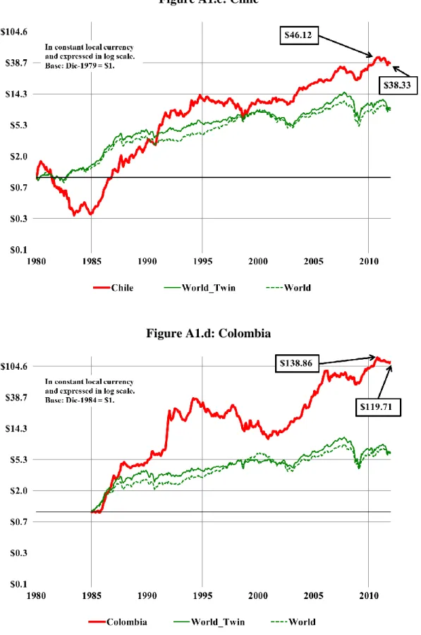
(15) A1.a-A1.g show the cumulative real returns of each country index starting from a value of 1 unit of domestic currency when the country enters the sample. S&P/IFC also provides the names of the stocks and the fraction of each national index capitalization at the end of each month that each one represents together with its industrial code at eight digits from the Global Industry Classification Standard (GICS). In some cases in the early years, only a handful of stocks made up the national index. To seek a minimum level of diversification, we incorporate each country in the sample in the month after 1979 in which it first appears with more than 10 stocks in the Global index. This starting date is a compromise between maximizing comparability of the results across countries and including a key regional event such as the start of the debt crisis in 1981. The first month in the sample is January 1980 for Chile and Mexico, November 1981 for Brazil, January 1985 for Argentina, Colombia and Venezuela, and January 1993 for Peru. The last observation for all countries is December 2011, with the exception of Venezuela which ends in March 2003.14 [Figure 1 about here] As it is standard in finance, we need to control for global conditions as reflected in the global market portfolio. In performing such a comparison, it is important to bear in mind that the industrial structure represented in emerging stock markets is much less diversified than that of the world index and it is substantially volatile both across countries and within countries over time. This is vividly shown by Figure 1 which reports the fraction of each index’s capitalization that is accounted for by stocks from each of the 10 industry groups that make up the first level of the Global Industrial Classification Standard. The graphs shows these data for the countries in the sample and for the whole world as measured by the S&P Global Broad Market Index (BMI) in 1990, 2000, and 2010. The numbers at the top of each bar report the weighted average sector participation (or Herfindahl index) for that country-year. The average Herfindahl index is 26% in Latin America while it is 13% in the world, so the Latin indices are on average about twice as industrially concentrated as the world index. The composition of the Latin indices is also more volatile. For example, the telecommunications sector went from being 2% of the Brazilian market in 1990, to 23% in 2000, and back to 3% in 2010, while in Mexico this sector went from 15, to 27 and to 34% over the same time period. By contrast, in the S&P Global BMI the weight of this industry group has oscillated between 2 and 5% over the same years. Moreover, sectors that are important in the world are underrepresented –or simply missing– in the Latin indices. For example the health care sector, which in the world represents between 8 and 12% of the market portfolio almost never appears among the Latin indices, while something similar happens with information technology.. 13. Because the price indices often take some time to reflect underlying inflation we used the average CPI inflation of months t, t+1 and t+2 in order to convert nominal returns of month t to real returns. For robustness we also ran the estimation using only the inflation of month t to deflate the month-t returns, but results are not significantly altered. 14 For Venezuela the available data actually go up to March 2007, but the prices after March 2003 seem unreliable so we dropped those observations.. 11.

(16) It is obvious from this discussion that the world index is not an appropriate comparison benchmark for the countries in the sample. We therefore build a twin index for each country, which is an index of global securities that match the industrial composition of each i country in each month. More specifically, if x t  1 is the vector of industry capitalization weights in the national index of country i at the end of month t-1, and R t  is the vector of world returns by industrial sector during month t, then the return on the twin index for country i during month t is, w. R w t   x t  11x 38 R t 38x1 i. i. '. w. (4). As noted in the introduction with the examples of Mexico and Peru in 2011, this turns out to matter substantially to interpret the source of stock market movements in the countries in the sample. Global returns of each industry are taken from the U.S. dollar-denominated Datastream Global Equity Indices which are grouped according to the Industry Classification Benchmark (ICB) at four digits –i.e. a slightly coarser partition than that provided by S&P/IFC for the national indices. We matched GICS and ICB codes using the description of each industry in the respective definitions. There are a total of 118 sectors that appear at least once in the Latin indices according to the GICS classification at eight digits, and they belong to 38 ICB sectors at four digits for which we obtain Datastream Global Equity indices. We used the US consumer price index to compute real returns for these global sectors. Besides including each country’s index, Appendix Figures A1.a-A1.g also show the S&P Global BMI index in real terms, a measure of an unconditional world market index, and the twin index for each country. The figures make clear why the twin indices provide a better benchmark than the standard world index. Take the case of Peru (Figure A1.f). From 1993 until 2000, Peru’s index rose from $1 to $2.17 while the world index rose from $1 to $2.54, so it would seem that Peru underperformed. However, during the same interval, Peru’s global twin index rose from $1 to $1.84, so Peru actually did much better than the world, holding industrial structure constant. By contrast, by October 2007, Peru’s twin index had risen to $7.28 while the world index had risen to only $3.56. Therefore, when judging the corporate value created during the Peruvian presidencies of the 1990s and the 2000s, it is critical to take into account how local conditions affect corporate valuations relative to the world, holding industrial risk constant. Otherwise, we would be underestimating the true relative performance during the 1990s and overestimating it during the 2000s. The figures for the other countries suggest a similar pattern: in general the global twin portfolios did worse than the world market portfolio in the 1990s and much better than it in the 2000s. The terms of trade (TOT) data are taken from national statistical offices and from Izquierdo et al. (2008), see the data section of the Appendix for details. For some countries these data are only available on a quarterly basis so we impute to each month in the quarter, the corresponding quarterly rate of change,. . . . . ~ ~ ~ TOT i t   ln TOT i t   ln TOT i t  1 ,. 12. (5).

(17) ~. where t denotes time as measured in quarters.15 The data section of the Appendix lists the presidents in the sample with each one’s election and inauguration dates and the specific sources used. When there is a two-round system, we used the month in which the election was defined (this could be the first or the second round) as the start of the presidency. In one of the robustness checks, the new president’s dummy begins three months before the date in the benchmark specification. The number of months in the sample for the presidents’ comparison varies between a minimum of 15 months and a maximum of six years with two exceptions.16 The Unit of Measurement Issue It is worth highlighting that in our benchmark specification the local return is measured in local consumption units while the return on the twin index is measured in US consumption units. We choose to do this mainly because we want to avoid declaring that a given administration generated much shareholder value during a certain period just because it allowed the value of the local currency to appreciate. However, in principle, it is not clear which route one has to take. To see this, notice that the return of a given country i measured in terms of consumption units of country i, which in logs we can call Rti ,i , differs from the return in that same country measured in consumption units of the US, Rti ,US , by the bilateral real depreciation rate, rerti ,US ; this is, Rti ,i  Rti ,US  rerti ,US .17 Suppose then a period in which the rate of return in US consumption units of the twin portfolio of country i equals i the return in country i’s consumption units of the local portfolio, i.e. Rti ,i  Rtw . In this case, our measure of excess return will equal zero. If, instead, we were to measure the domestic portfolio in US dollars, the excess return will equal the real appreciation, i.e.. 15. When we do have monthly data we just take its value at the end of each quarter and proceed as above. The exception to the maximum duration is Pinochet whose first presidency ended in February 1981 and whose second term ended with the election of President Aylwin in December 1989. Given that our data only start in 1980, we bundle both presidencies under a single Pinochet period from 1980 until November 1989 for simplicity. Similarly, Cristina Kirchner’s dummy remains on after her reelection in October 2011 and until the end of that year. The exception to the minimum duration is President Humala of Peru who enters the sample in May 2011 and for whom we report the return decomposition during his seven months in the sample only for illustrative purposes. When a president was followed by the next in line of succession without a general election, the new president’s sample period begins on the month that he or she took office. A few months in the sample are dropped in the presidents’ comparison. For Argentina, December 2001 is dropped since President de la Rúa resigned on December 20 and there was a sequence of presidents from the line of succession until the situation stabilized in early 2002 when President Duhalde was appointed by Congress. For Peru, President Paniagua, who was in office from November 2000 until May 2001, is also dropped. For Venezuela, Presidents Lepage and Velázquez, who were in office from May until November 1993, are dropped. 17 Notice that if relative PPP were to hold, measuring returns in local or foreign consumption goods will be the same. While it is probably not reasonable to assume that PPP will hold in the short run, given that we are interested in the average return during a presidential mandate of around four years, relative PPP might not be a bad approximation. 16. 13.

(18) Rti ,US  Rtw  Rti ,US  Rti ,i  rerti ,US . Thus, in this case a real appreciation of the domestic currency would be taken to be a positive national contribution. i. Alternatively, imagine a period in which the rate of return in US consumption units of country i’s twin portfolio equals the rate of return in US consumption units of the local portfolio, i.e. Rti ,US  Rtw . If we were measuring country i’s return in US consumption units, there would be no local contribution, but if we were measuring the country i’s returns in local consumption units (as in our benchmark case) we will be declaring a positive local contribution when there is a real devaluation. Given these possible measurement differences, we report the results using local consumption units in the baseline specification and then include the results using US consumption units in the robustness section. As it turns out, the results are quite similar with the exception of a few presidencies during which large real exchange rate depreciations took place. i. 4. Empirical Model and Results We present the methodology and the results in four subsections. In the first one, we describe how we compute the global and regional factors and characterize how they have evolved over time. In the second one, we compare the performance of the different countries over the whole sample. In the third subsection we compare presidential periods in each country. Finally, we present several robustness exercises in the last subsection.. 4.1. The global and the regional factors We first identify the global and regional effects throughout the whole sample. The dependent variable is the monthly difference between the local and the twin index return, Ri t   R w t  . We identify the regional factor by allowing for a yearly time dummy. We i. also control for the change in each country’s terms of trade, TOT i . As noted by LevyYeyati and Cohan (2011), variations in Latin American terms of trade display important commonalities across countries. Such common movements will be reflected through the coefficient on the time dummy. Therefore, the coefficient on TOT i will only pick up the country specific variation in terms of trade. The empirical model is,. R t   R i. wi. 2011. t     TIME t   . TOT i t    i t .  1980. (6). t  Jan  1980,..., Dec  2011, i  1,..., 7. 14.

(19)  where TIME t  is a dummy variable equal to one if month t belongs to year.  .18 We first. assume that the incidence of TOT i is the same for all countries, but we relax this assumption in the robustness section. The model is estimated by OLS with White-robust standard errors, which yields consistent estimates under the small-open economy i i assumption (i.e. that R w t  and TOT t  are strictly exogenous). This type of model has been frequently used in the finance literature to identify industry effects in major equity markets as well as country and regional effects by e.g. Heston and Rouwenhorst (1994), Baca, Garbe, and Weiss (2000), and Brooks and Del Negro (2004). Our regression is equivalent to including the twin portfolio on the right hand side with a coefficient equal to one. This specification is justified by the goal of our paper, which is to assess how domestic conditions affect corporate value relative to average conditions in the rest of the world, holding industrial risk constant. That is exactly what the difference. R i t   R w t  reports. This contrasts with the traditional finance literature that attempts to gauge the ability of the domestic portfolio to diversify the risk embedded in the world market portfolio. In other words, our approach is like comparing the choice of living (and producing) in a given country to living in the “twin” country, and in this choice the ability to diversify risks is irrelevant (either one lives in a country or not). We think that this is the appropriate choice given the goal of the paper, although it is not characterizing diversification opportunities. i. Following this estimation, the global contribution for country i during month t is, i Rˆ Global,i t   R w t   ˆ TOT i t  ,. (7). the regional contribution is the same for all countries,. Rˆ Regionalt   ˆ | t. (8). and the national differential contribution is simply the residual, Rˆ National Differential,i t   ˆ i t  .. (9). Table 1 summarizes the results. For completeness we report in straight case the results from i the model that does not control for TOT and in italics those that do, but for the sake of 18. The model without TOTs uses monthly observations, while we use quarterly observations in the one that does control for TOTs.. 15.

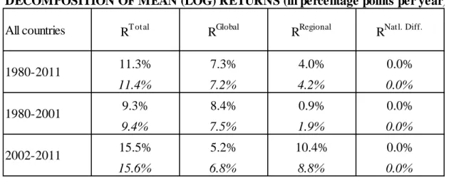
(20) space here we discuss only the results that do include them.19 The top panel reports mean returns and the bottom one focuses on the volatility of returns. Over the whole sample period, Latin American stocks grew at an average 11.4% per annum compared to 7.2% for the twin portfolio, so they surpassed their benchmark by 4.2% per year.20 However, this over performance is concentrated in the latter period: Latin American stocks surpassed their benchmark by about 1.9% per annum during 1980-2001, while they over performed by almost 9% during 2002-2011.21 So the notable Latin American performance is a relatively recent phenomenon, and is not due to higher returns of the twin portfolio, which were even smaller during the latter period.22 [Table 1 about here] The bottom panel deals with volatility. The left column shows that the standard deviation of total annual returns has fallen from 49% during 1980-2001 to 33% since 2002, a substantial reduction. The three columns to the right show the decomposition of total return variance in the fractions associated with its three components from equation (3). 23 Over the whole sample period 0.54 of the variance of returns stems from purely national sources. Until 2001, 0.92 of volatility resulted from the regional plus the purely national factors, while since 2002 these factors amount to only 0.3 of total volatility.24 We attribute the corresponding rise in comovement with the world to greater commercial and financial integration since 2000. The key figure in this table however is the huge reduction in the fraction of volatility associated with the regional shocks which fell from 0.31 to 0.05. The two panels taken together suggest that the main driver of differential results between 1980-2001 and 2002-2011 was the regional contribution, which increased almost six fold from the early to the latter part. Moreover, it was also much more stable: it went from about one-third of the total return volatility to about one-twentieth. The ratio of mean annual. 19. In the rest of the paper we focus on the model that does control for TOTs. The results from the other model are similar and are available from the authors on request. 20 All figures are in percentage points per annum. 21 This (arbitrary) cutoff date is chosen to highlight the extraordinary performance of the last decade as noted in the introduction. 22 Given that we are allowing for yearly effects, the sum of the residuals across countries within a year has to be zero and that is what the right column shows. The mean residual for the different countries and presidential terms periods is the subject of the next sections. 23 Given that the regional factor is only available at annual frequencies, in order to compute variances and covariances, we first add up the monthly components of equation (3) within each calendar year. In order to express returns on a common scale, we next discard all country-years which lack a full 12-month record of returns –otherwise, we would be underestimating the variance of the regional component. The statistics shown in the bottom panel of Table 1 are computed off the resulting dataset. For the computation of the variance ratios, we assume that the order of causation goes from the global to the regional and from there to the idiosyncratic shock. Hence, the covariance between these variables involving the global shock is attributed to it, and the covariance between the regional and the idiosyncratic shock is attributed to the former. 24 The rise in importance of global volatility was true even before the Lehman crisis: 0.37 of the total variance was associated with that of the twin portfolios from 2001 until 2007, while it was 0.04 during the previous 21 years.. 16.

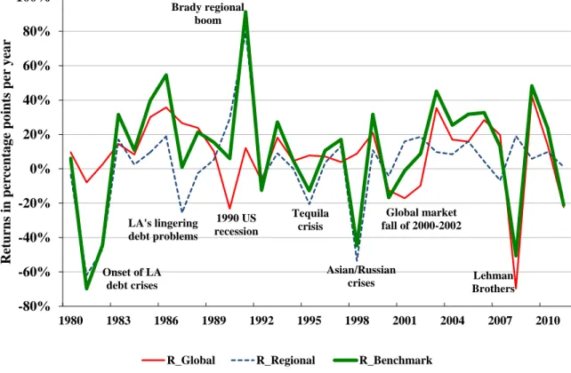
(21) return over standard deviation of annual return for the regional contribution went from near 0.07 in 1980-2001 to almost 1.2 in the last decade, a huge improvement.25 It is useful to compare these results with the literature that seeks to gauge the effect of external factors on the macroeconomic performance of emerging countries, focusing on variables such as GDP, consumption and inflation, as reviewed above. The general message of these studies is that external shocks are key sources of fluctuations in emerging countries, explaining between 25 and 50 percent of the volatility of output. Using a different approach González-Rozada and Levy-Yeyati (2008) study the influence of external factors on emerging market spreads and find that they account for between 20 and 40% of their total variance. Along similar lines, for the whole sample we find that 49% of the variance of local returns is explained by global and regional factors. Moreover, we also document how the role of these factors has evolved over time. In particular, the global factor has become much more influential while the regional factor has become less so in explaining domestic volatility. This is exactly what one would expect as economies become more integrated into the world. [Figure 2 about here] Figure 2 plots the evolution over time of the cross country average of the yearly Global contribution, the Regional contribution, and the sum of both.26 As expected, this very simple decomposition pinpoints critical times for the region such as the onset of the debt crisis in 1981-82, the emergence of it through the Brady plan (1991) and the contemporaneous spike of capital inflows discussed by Calvo et al. (1993), the Mexican (Tequila) crisis in 1994, the Asian and Russian crisis of 1998, the Lehman Brothers crisis in 2008, and the more recent global events driven by the European sovereign debt crisis, among others. Although the regional contribution was the most volatile component of the two in the early period –with extremes of -69% in 1981 and 78% in 1991–, it has hovered in a relatively smooth range –bounded by -6% in 2007 and 22% in 2002– since 2001. As noted in Table 1, the most volatile contribution of the last decade has been the global contribution. It is also instructive to compare the sum of our global and regional factors to the Brookings Global Wind Index (GWI)27 constructed by Levy-Yeyati and Cohan (2011). While the overall evolution of both indices is quite similar, some differences arise. For instance, according to their measure the world continued to be favorable to Latin America during 2011, while our figures display a marked decrease. This highlights the conceptual difference between relying on asset prices and on GDP. Since our measure is forward 25. This is known in finance as the Sharpe ratio and it is a widely used measure of risk-adjusted performance in finance. 26 These are estimated from the monthly regression that includes TOTs, but results are very similar without them. Appendix Table A1 reports the estimated coefficients and their standard errors for both specifications. The global contribution that we estimate in (7) is a monthly series, but for simplicity we base this figure on the yearly sum thereof. 27 This is a synthetic index characterizing the evolution of external conditions based on information from local GDP growth, a risk index, commodity prices and global growth. Their sample consists of the same countries as ours, minus Venezuela plus Uruguay.. 17.

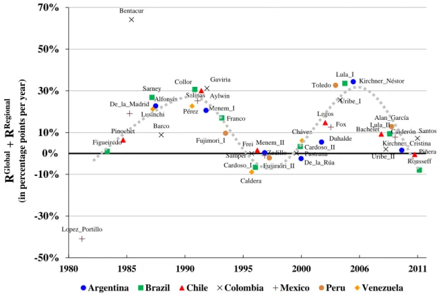
(22) looking, it anticipates the problems that the world might face in the near future (e.g. as the European sovereign debt crisis and the risks to global growth evolve). The GWI on the other hand is relatively more backward looking and captures that GDP growth was still high in most Latin American countries throughout 2011. In spite of these differences, both indices explain roughly similar fractions of total variance. The GWI explains almost 90% of Latin American growth variance since the year 2000. As noted in the last line of Table 1, our global plus regional factor (our analog of the GWI) explains about 75% of observed return variance over a similar period. [Figure 3 about here] The vertical axis in Figure 3 depicts the average global plus regional shock that each T. Rˆ Global,i t   Rˆ Regionalt . t 1. T. president faced, expressed in annual units of log returns, 12. ,. while the horizontal axis shows the midpoint of his or her term in office. Three points are worth noting in this figure. First, while there are important differences in industrial composition of the twin portfolios across countries, benchmark conditions for presidents in office in similar times are actually quite similar. Second, there is a markedly recurring cyclical pattern of benchmark conditions over time. Third, the gap in benchmark conditions between good and bad times is substantial: Presidents that faced benign international environments experienced benchmark returns of up to 34.4% per year, which amount to a 295% stock market appreciation over a hypothetical four-year presidency.28 At the other end, presidents that faced difficult international environments experienced benchmark falls in asset prices of about 9% per year which amount to a cumulative reduction of about 30% in stock prices.29 Furthermore, as noted in the introduction, the countries in the sample have applied very different policies in the cross section over the last 10 years, but all of them have achieved much more impressive national results than in the previous 20 years. Figure 3 suggests that such presidencies as Néstor Kirchner’s in Argentina, Lula da Silva’s (I) in Brazil and Alejandro Toledo’s in Peru experienced a period of very favorable benchmark conditions. In the polar case in which the benchmark return is interpreted as external windfall, the abundance of the presidencies centered around 2006 might be more related to the bonanza of this global environment than to the domestic policies themselves.. 4.2. Comparing Countries We next assess which countries in the region faced higher benchmark conditions and which have had a greater differential performance during sample. Table 2 reports the results. [Table 2 about here] 28. That benchmark return corresponded to Nestor Kirchner’s presidency which lasted 54 months so the cumulative benchmark return was actually 369% as reported in Table 3.a. 29 We are excluding the two outliers Betancur and López Portillo since our time series only cover a fraction of their presidencies. Benchmark returns would be much more extreme if we were to include them.. 18.

(23) The left panel reports the average annual total return, and its decomposition in benchmark and national differential returns by country. The benchmark return is the sum of the global and regional returns from equations (7) and (8). From equation (3), the total return in the left panel is the sum of the different components of returns. Overall, the sum of global plus regional average shocks explains an average stock market appreciation of between 8.4 and 14% per year depending on the country. Argentina, Colombia and Brazil were the countries that had the best benchmark returns during the sample, while Venezuela, Mexico and Chile faced the worst external conditions. Much of this difference in external conditions is attributable to the time of entry into and exit from the sample. For example, Chile and Mexico display low values of benchmark conditions in part because they were the only countries in the sample during 1981, a year in which the regional shock had a -71% performance. Venezuela entered the sample in 1986 so it avoided the very bad 1981-82 years, but it exited the sample in 2003 and so it also avoided the very good years of regional contributions thereafter. Other differences may result from industrial composition of the national index and from idiosyncratic shocks to terms of trade. It is evident then that benchmark conditions were not uniform across countries and this is important in assessing the overall performance of measured returns. The benefit of our methodology is precisely that it can purge whatever are the measured total returns of this world or regional components and focus on each country’s differential contribution. In other words, the measured global and regional returns only make sense as a benchmark against which to compare actual country returns. The table suggests that the best national differential return performers were Peru (4.1% p.a.), Colombia (4% p.a.) and Chile (1.5% p.a.) and that the worst performers were Argentina (-4.9% p.a.) and Venezuela (-6.8% p.a.). It is instructive to look at the accumulated returns from each source during each country’s presence in the sample, which is done in the right panel of Table 2. The first column in the right panel reports the cumulative wealth from having invested 1 unit of consumption goods in each country when it entered the sample and holding it until the end.30 Since we use continuously compounded average annual returns in the left panel, numbers in the corresponding column of the right panel are e ( R*T / 12) , where T is the number of months that each country is in the sample. They show the cumulative returns from each source: the global returns, the regional returns and the national differential returns. Therefore, negative numbers in the left panel are coupled with a number lower than 1 in the right panel. The total wealth in the right panel is the product of the different source of returns times the hypothetically invested $1. The results from this exercise are impressive. The benchmark portfolio for Colombia during its 27 years in the sample rose from 1 to 41 consumption units, while the Colombian stock index rose from 1 to 120 consumption units, almost tripling the benchmark returns. Peru’s control portfolio rose from 1 to 8.45 consumption units but the Peruvian index rose from 1 to 18.5 during its 19 years in the 30. As discussed in the data section we use local consumer price indices for the Latin American returns and US CPI for the twin indices. Hence the monetary units of the right panels of tables 2 and 3 are purged of inflation.. 19.

(24) sample; hence it more than doubled the benchmark returns. Chile was in the sample during 32 years, which included the early 1980s debt crisis, so it had lower own and benchmark performance. Overall, its benchmark world portfolio appreciated from 1 to 24 consumption units, while its national index rose from 1 to 38, 1.6 times the benchmark. By contrast, Argentina’s benchmark portfolio appreciated from 1 to 37.2 consumption units, while the national index rose from 1 to only 10.6 consumption units, hence the national differential performance cumulated to multiplying the benchmark return by a factor of 0.28. In a similar pack, during its 19 years in the sample Venezuela’s control portfolio rose from 1 to 4.1 consumption units, but the Venezuelan index national rose from 1 to 1.32 consumption units, hence multiplying the benchmark return by 0.32. These accumulated national differential returns are sizable figures. In financial terms, they mean that the stock markets of those countries have returned much more (less) compared to a world benchmark that has the same industrial composition, equally affected by each country’s change in terms of trade and equally exposed to regional factors. If we interpret the national differential over these long periods as capturing the long term effects of the quality of domestic policy from the viewpoint of equity investors, our model suggests that there have been significant differences in policy quality across countries.. 4.3. Comparing Presidents We next use the model to analyze the performance of different presidential administrations. In this case, for every president, we compute the average of each contribution (j) to total returns in his or her country (i) from the month in which that president became elected until the month before the new president became elected, and express it in annual units,.  . T. Average R j ,i  12  t 1. R j ,i t  , T. (10). where j = global, regional and national differential returns. Since the model has a yearly time effect, the sum of all the country residuals (i.e. the national differential contributions) in equation (6) has to be zero each year. Hence, the model essentially runs a contest among the presidents in office in each year, using the estimated residuals from (6) as a proxy for their (demeaned) contributions, since the mean contribution goes to the regional factor. It then sums these residuals and computes the annual average which is reported as the national differential contribution. As mentioned before, it is important to bear in mind that the chance that our measure of presidential performance is affected by events unrelated to policy (e.g. natural disasters, unusual weather, local bubbles, etc.) is larger the smaller the sample size, hence our cap of a minimum of 15 months in the sample for the presidents’ comparison. A similar sampling error problem occurs with many other tests –be it in a university course or in a clinical setting. Our goal is to provide a not systematically biased benchmark against which. 20.

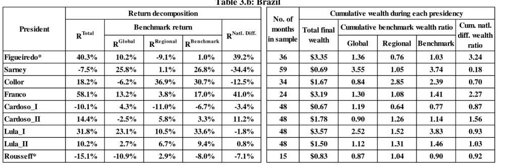
(25) economic outcomes during a presidency can be compared. We next review each country in turn. Tables 3.a-3.g report the results by country, following the same structure as Table 2.31 [Tables 3.a – 3.g about here] Argentina: Table 3.a shows that Néstor Kirchner faced a global plus regional return of 34.4% p.a., the greatest benchmark bonanza per year among all the presidents in the sample.32 As shown in the right panel of Table 3.a, when cumulated over his 54 months in office, this gives a total benchmark appreciation from $1 to $4.69. The national differential return during his mandate was -4.7% p.a. which gave a cumulative national differential wealth ratio of 0.81. This means than investors in Argentina during his presidency increased their wealth from $1 to $3.79 (= $1 x 4.69 x 0.81), so in total Argentina yielded 29% less than the benchmark. Contrary to the claims of many analysts, Cristina Kirchner did not face a period of worldwide prosperity: her benchmark return was a meager 1.5% p.a. which gave a cumulative wealth ratio of 1.07 during her first 51 months in office; still larger than Menem’s second term (cumulative benchmark wealth ratio of 1.01). The president with the largest national differential contribution was Duhalde with 19.1% p.a. followed by Menem’s second term at about 12% p.a. De la Rúa and Alfonsín had very negative national differential contributions of about -38% and -15% p.a. respectively, which gave cumulative national differential wealth ratios of 0.63 and 0.44 respectively.33 Menem’s first term, Néstor Kirchner and Cristina Kirchner all displayed negative national differential returns.34 Brazil: Table 3.b shows that Collor de Melo and Lula’s first term faced the highest benchmark conditions, with regional plus global shocks greater than 31% p.a. At the other extreme, Dilma Rousseff faced a negative benchmark return of -8% during her first 15 months in office while Cardoso’s first term faced the Tequila crisis, the Russian and the East Asian crises in 1998, for an overall average negative benchmark return of -6.7% p.a. The president with the largest national differential was Itamar Franco (41% p.a. during the 24 months of his term in the sample) under whose presidency then Minister Cardoso implemented the Real plan that ended hyperinflation. The other successful presidents 31. Presidents for whom our sample does not cover their full tenure in office are marked with an *. Since a few months are dropped from the sample in the presidents’ comparison, the vertical multiplication of cumulative wealth in Tables 3.a-3.g has minor discrepancies with that same variable reported for the full country time series in Table 2 in the cases of Argentina, Peru and Venezuela. See data section for details. 32 Here we are excluding Colombia’s Betancur (an outlier) since our sample covers only a fraction of his presidency. We use this return to construct the hypothetical good-state of the world return during a typical four-year presidency reported in the abstract and in the introduction: e 0.344 x 4-1= 295%. Nestor Kirchner is actually in the sample for 54 months, but we standardize those extreme benchmark conditions for typical fouryear long presidencies. 33 Argentina’s bankruptcy law was amended at the beginning of Duhalde’s presidency in a way that favored equity holders at the expense of bondholders. As noted in section 2.1 this is one case in which our measure can be affected by the presence of distributional effects. Furthermore, Duhalde is one of the few cases in which the results change significantly if we measure returns in real US dollars. See the robustness section for details. It is important to keep in mind that our Argentina sample starts in January 1985, so this computation is missing the first part of Alfonsín’s presidency. 34 Some months are not assigned to any president (e.g. Dec-2001 in Argentina, Nov-2000 until May-2001 in Peru, and from May until Nov-1993 in Venezuela), hence the vertical multiplication of cumulative wealth in Tables 3.a-3.g has minor discrepancies with that variable reported for the full country time series in Table 2.. 21.