Prediction of single salt rejection in nanofiltration membranes by independent measurements

1 2 3 4 5 6 7 8 9 10 11 12 13 14 15 16 17 18 19 20 21 22 23 24 25 26 27 28 29 30 31 32 33 34 35 36 37 38 39 40 41 42 43 44 45 46 47 48 49 50 51 52 53 54 55 56 57 58 59 60 61

Prediction of single salt rejection in nanofiltration

membranes by independent measurements.

Verónica SILVA1, Miguel MONTALVILLO1, Francisco Javier CARMONA2, Laura PALACIO1, Antonio HERNÁNDEZ1 and Pedro PRÁDANOS1*

1

Grupo de Superficies y Materiales Porosos, Dpto. Física Aplicada, Facultad de Ciencias, Universidad de Valladolid, 47071Valladolid, Spain

2

Dpto. de Física Aplicada. Escuela Politécnica, Universidad de Extremadura, 10004 Cáceres, Spain

*E-mail: [email protected]

Abstract

In this work a method is proposed to predict salt rejection by nanofiltration. The procedure starts from the steric, electric and dielectric exclusion model with charge (and permitivity) depending on the concentration along the pore, SEDE-VCh, for membrane characterization, and substitutes all fitting parameters by values obtained by independent methods. These parameters are the relative permittivity inside the pores and the two constants of the Freundlich isotherm for the volumetric charge density, which can be obtained by impedance spectroscopy techniques. Moreover, the pore size and shape and the active layer thickness are required to complement the model. The pore size was obtained by using a neutral solute rejection test and the active layer thickness was estimated by SEM. Therefore, the model also requires pore shape as input. AFM measurements suggest the assumption of a slit shape for the pores.

A Desal-HL membrane has been structurally, electrically and functionally characterized. These data allowed the testing of the predictive model that was subsequently demonstrated; as far as results are good enough considering the complexity of the mechanisms involved. Consequently, it seems clear that once the model parameters have been obtained by independent methods, it can be used as a predictive tool.

Keywords: Impedance Spectroscopy, Nanofiltration, Membrane Potential, Transport numbers, Dielectric properties

*Manuscript

1 2 3 4 5 6 7 8 9 10 11 12 13 14 15 16 17 18 19 20 21 22 23 24 25 26 27 28 29 30 31 32 33 34 35 36 37 38 39 40 41 42 43 44 45 46 47 48 49 50 51 52 53 54 55 56 57 58

1. Introduction

Nanofiltration (NF) membranes possess some special characteristics that distinguish

them from ultrafiltration (UF) and reverse osmosis (RO) ones. Firstly, they keep relatively

high permeate flux at low pressure operation compared with conventional RO [1], and

secondly, most of them are electrically charged with the subsequent effect on the solute

separation mechanism.

Due to the clear interest of NF, it is desirable to have a way to estimate the

performance of NF membranes for different solutes and/or combinations of solutes in order

to have a predictive understanding of their behavior. As a consequence, there have been many

efforts, with this aim in mind, focusing on the development and optimization of mathematical

models to predict the separation properties of NF membranes. Firstly based on irreversible

thermodynamics (Kedem, Katchalsky and Spiegler works) [2, 3], continuing with the

hydrodynamic model or pore model introduced by Ferry [4], and the development of

hydrodynamic approach models based on the extended Nernst-Planck equation such as the

steric hindrance pore, SHP, [5], Teorell-Meyer Sievers, TMS, [6, 7], the space charge model,

SCPM, by Wang et al.[8] and more recently the Donnan steric partitioning model, DSPM,

which combines the steric and Donnan exclusion effects [9].

Nowadays the most complete models include dielectric exclusion effect [10],

including steric, Donnan and dielectric partitioning effects in the interfaces and convective,

diffusive and electromigrative transport effects in the inner part of the membrane. The mass

transfer through the membrane is described using the extended Nernst-Planck equation

modified by hydrodynamic coefficients to reflect the influence of the pore constriction on

1 2 3 4 5 6 7 8 9 10 11 12 13 14 15 16 17 18 19 20 21 22 23 24 25 26 27 28 29 30 31 32 33 34 35 36 37 38 39 40 41 42 43 44 45 46 47 48 49 50 51 52 53 54 55 56 57 58 59 60 61

[1]. These effects are the Donnan exclusion and the dielectric exclusion, being the later

composed by two terms, the Born effect and the image forces one. The Born effect is

connected with the low values of the relative permittivity of a liquid inside a pore of

nanometer dimensions. The image forces effect correspond to the interaction between the

ions and the polarization charges induced by them at the pore wall.

Bandini in 2001-2002 firstly presented the Donnan steric partitioning model with

Dielectric exclusion model, DSPM&DE, [11]. It is a model in which the ionic partitioning at

the interfaces between the membrane and the external phase takes into account the three

separation mechanisms: steric, Donnan equilibrium and dielectric exclusion. Bandini’s model

introduced the idea of the dielectric exclusion as an additional cause of partitioning to those

of bare Donnan steric pore model (DSPM) initially proposed by Bowen [9, 12, 13]. We refer

to the reading of the work of Bandini for a more extensive explanation of the model [14].

In 2005, Szymczyk and Fievet proposed another model, the steric, electric and

dielectric exclusion, SEDE, model [15]. The volume charge density of a NF membrane was

determined from tangential streaming potential measurements (TSP) and the model was used

to assess the rejection rate of the membrane with a single adjustable parameter: the relative

permittivity of the solution filling the pores. In a later work [1] Lanteri et al. proved that the

SEDE model is able to reproduce both experimental rejection rates and membrane potentials

by using several fitting parameters: effective pore size, effective thickness-to-porosity ratio,

a ka

x A , effective volume charge density, X, and relative permittivity inside the pores, _p,

all them being considered constant through the membrane. Unfortunately, it was observed

that there are different couples of values (X , _p) that lead to the same membrane potential

value, between all of them, true values of X and _p are difficult to obtain by any fitting

1 2 3 4 5 6 7 8 9 10 11 12 13 14 15 16 17 18 19 20 21 22 23 24 25 26 27 28 29 30 31 32 33 34 35 36 37 38 39 40 41 42 43 44 45 46 47 48 49 50 51 52 53 54 55 56 57 58

[16], Déon et al. assumed the model proposed by Silva et al. [17] that considered that the

charge density within the pore varies with concentration. Déon et al. did not included the

image force term into the dielectric effect. However they assumed that this effect would be

indirectly included in the "effective" estimated value for _p that can be obtained by fitting but

that sometimes lead to weird values.

This article presents a novel method to predict the salt rejection developed by a NF

membrane. The model includes three parameters: the relative permittivity inside the pores,

p

 , and the  and Γ parameters of a Freundlich charge isotherm of the volumetric charge

density, X c . Unlike the papers presented so far, in the present work these three

parameters are obtained by independent methods or experimental techniques.

In this case, an estimation of the thickness of the active membrane layer, x_a, is

obtained from scanning electron microscopy, SEM, allowing the evaluation of membrane

porosity, A_k, from water permeability measurements. The membrane porosity of the active

layer is necessary to link the relative permittivity of the wet membrane with the

corresponding value for the solution inside the pores and the dry membrane material, as it

will be explained later. Transport numbers are obtained from membrane potential

measurements. The viscosity inside the pore is calculated by using only the pore radius and

the bulk value. In the present work, as it was done previously [17], the volumetric charge

density and the relative permittivity inside the pores were considered as variable along the

pores and depending on concentration, _p  f c( ) X f c ( ). These two magnitudes are

obtained from Impedance Spectroscopy (IS) measurements using a similar method to that

described previously [10]. The model can be called SEDE-VCh model because it uses steric,

1 2 3 4 5 6 7 8 9 10 11 12 13 14 15 16 17 18 19 20 21 22 23 24 25 26 27 28 29 30 31 32 33 34 35 36 37 38 39 40 41 42 43 44 45 46 47 48 49 50 51 52 53 54 55 56 57 58 59 60 61

consequently on distance along the pore). The changes of charge along the pore, within this

model, can be as large as to span over an order of magnitude, depending on the operation

conditions and leads better fitting to the experimental results [17].

The main objective of the present work is to evaluate the predictive capacity of the

model to foretell NF performances. The predictive character of the model consists in its

ability to obtain retention from independently known morphological and electrical properties

of the membrane. This permits securing the proposed model as to get membrane retention by

easier and faster procedures tan the simple measurement of observed retention followed by a

careful concentration-polarization through mass transfer models. With this aim, the

experimental volume flux and intrinsic retention of aqueous NaCl solutions through a flat

sheet Desal HL, a polyamide NF membrane made by GE-Osmonics, will be compared with

the corresponding predictions obtained from independently measured _pand X. It will be

shown that fair accordance is found for the concentrations range studied.

Desal HL is a typical composite membrane, it consists of three layers: a thin top

selective polyamide layer of a few hundred nanometers in thickness

(poly(piperazine-amide)), an asymmetric microporous polysulfone support layer, and a polyester non-woven

fabric layer for mechanical strength [18, 19]. This membrane has been studied in our previous

work [10, 20-22] and others authors [18, 19, 23, 24] so there is a good reservoir of knowledge

on its characteristics and functionality that can help to assess the models and its predictive

capacity.

2. THEORY

2.1. Dielectric Analysis

Impedance spectroscopy measurements determine the electrical impedance of a

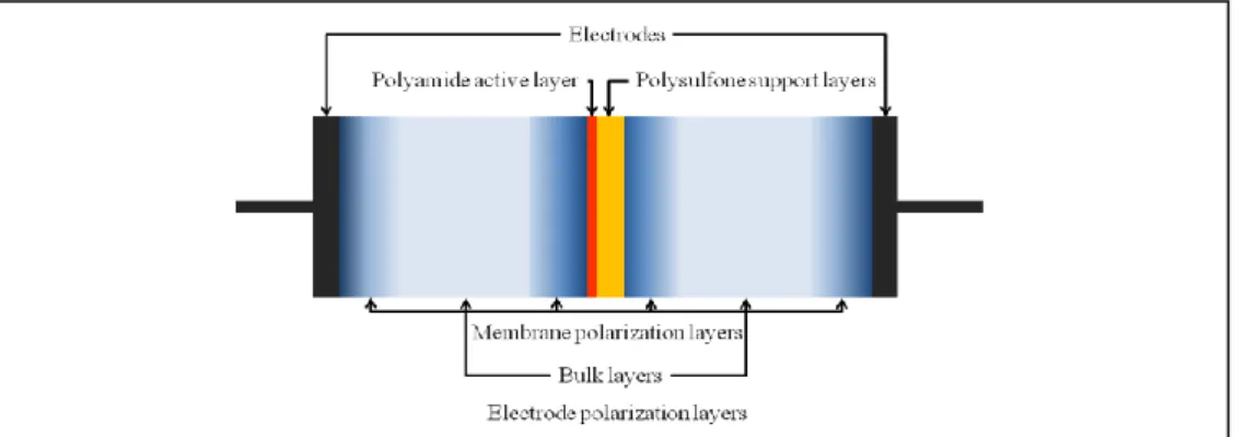
1 2 3 4 5 6 7 8 9 10 11 12 13 14 15 16 17 18 19 20 21 22 23 24 25 26 27 28 29 30 31 32 33 34 35 36 37 38 39 40 41 42 43 44 45 46 47 48 49 50 51 52 53 54 55 56 57 58

membrane, the system is formed by five elements or layers: electrode + electrolyte +

membrane + electrolyte + electrode. The system corresponds to three phases: electrode,

membrane and electrolyte. In such a system it is possible to recognize a scheme of series

resistance as shown in Figure 1. Evidently similar layers can be characterized by a unique set

of electrical parameters or elements.

For the dielectric analysis, we follow the same procedure than in our previous work,

in order to analyse the Impedance Spectroscopy results [10, 21]. A summary of the procedure

followed can be found in the Appendix A.

2.2. Relative permittivity and conductivity inside NF pores

The relative permittivity of the wet membrane,_memb(as obtained from Equation

(A.8) in Table A.1) can be split as a linear combination of two terms, the permittivity inside

the pores, p, and the membrane dry material permittivity, d, as,





memb pAk a d 1 Ak a

    (1)

The same relation is applicable for the overall or wet conductivity, _memb:





memb pAka d 1 Aka

    (2)

1

Where Akais the porosity of the membrane active layer. Aka can be estimated from

a ka

x A

 if the mean membrane thickness is known. This ratio can be obtained from the

Hagen-Poiseuille equation assuming slit pores and viscosity correction [25] as,

2

effect has been calculated for slit-shaped pores as proposed by Wesolowska [25]:





experimentally confirmed as discussed by Bowen and Welfoot[26, 27].

2.3. Thermodynamic equilibrium at the interfaces

Due to the nature of the impedance spectroscopy measurements, there is neither any

applied pressure nor any concentration gradient between both sides of the membrane. The

corresponding profiles in both impedance spectroscopy and permeation experiments are

1

Consequently the only mechanisms causing separation of the electrolyte are those

related to the thermodynamic equilibrium in both interfaces which are can be calculated as

account the steric effect,  represents the normalized Donnan potential, and the dielectric

effects are considered thorough the Born term, W'i,Born [28], and the image forces effects

Changes in conductivity from inside to outside the membrane can be correlated with

the equilibrium conditions as done in a previous work [10] through the following relation:

Figure 2: Scheme of concentration profile in the pores of the active layer of the membrane, a) on the experiences of Impedance Spectroscopy, b) on the experiences of

1

Where _i is a coefficient grouping the influence of steric and dielectric effects and

can be written as:

numbers inside and outside the membrane, respectively. Transport numbers are known to

represent the fraction of the total current carried by the positive and negative ions.

It is well-known that the adsorption process of ions in NF membranes can be

successfully described by a Freundlich isotherm [31, 32].

X_c

(8)

Substituting this isotherm into Equation (6), we get:



 

1 2 3 4 5 6 7 8 9 10 11 12 13 14 15 16 17 18 19 20 21 22 23 24 25 26 27 28 29 30 31 32 33 34 35 36 37 38 39 40 41 42 43 44 45 46 47 48 49 50 51 52 53 54 55 56 57 58

2.4. SEDE-VCh model for NF experiments

The SEDE-VCh model is the most complete approach based on the Nernst-Planck

extended equation [12, 33-35] and is our aim here, as mentioned, to test its predictive

features. In previous works, we demonstrated that the SEDE-VCh model can be used for the

electrical characterization





and also for multi-component mixtures with a common ion [22].

One of the major uncertainties in the characterization of a NF membrane is the

geometry of the cross section of the active layer pores. In most papers, authors assume two

ideal situations: pores with cylindrical section or pores with slit shape [22, 36]. In other cases,

authors go for only one of the two geometries based on preceding knowledge from several

characterization techniques [37, 38] or by fittings when mass transfer models are used [15,

39]. The model can be applied for cylindrical and slit pore geometries however, when

cylindrical geometry was assumed, some unusual values of p were found in the literature

(bigger than _w= 78.5) [17, 40] (both effects, Born and “images forces”, were taken into

account). When slit pore geometry is assumed, most of the results found in literature are in

better agreement with what could be expected giving, in particular, dielectric constants inside

pores below the water bulk value





been found when the charge density is evaluated from other techniques [41]. In the present

work, the use of slit geometry is supported also by the AFM results in the membrane Surface,

as will be explained in section 4.1.

To summarize the SEDE-VCh, we listed below the basis of the model together with

the list of equations involved presented in appendix B (Table B.1).

i. Slit-shapes pores

1 2 3 4 5 6 7 8 9 10 11 12 13 14 15 16 17 18 19 20 21 22 23 24 25 26 27 28 29 30 31 32 33 34 35 36 37 38 39 40 41 42 43 44 45 46 47 48 49 50 51 52 53 54 55 56 57 58 59 60 61

iii. Variable volumetric charge density along the pores.

iv. Image charges forces effects and Born effects are considered.

v. No dielectric effects are considered due to dispersion interaction occurring between

ions within pores and the membrane material [42], following most of the authors

who use these models [43].

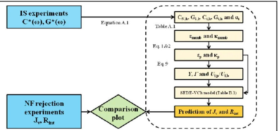
In Figure 3, a scheme of the procedure of evaluating the predictive power of the

model is shown.

3. EXPERIMENTAL

3.1. Membrane.

A flat sheet commercial NF membrane Desal HL has been used. This is a polyamide

membrane manufactured by GE-Osmonics (Minnetonka, MN, USA). According to the

manufacturers, it has a MWCO between 150 and 300 g/mol, and it can be used in a pH range

of 3-9 and up to a maximum temperature of 50ºC.

3.2. Atomic Force Microscopy (AFM).

Atomic Force Microscopy has been performed with a Nanoscope Multimode IIIa

scanning probe microscope from Digital Instruments (Veeco Metrology Inc., Santa Barbara,

CA, USA). As phase images show surface features with greater clarity than the height image

1 2 3 4 5 6 7 8 9 10 11 12 13 14 15 16 17 18 19 20 21 22 23 24 25 26 27 28 29 30 31 32 33 34 35 36 37 38 39 40 41 42 43 44 45 46 47 48 49 50 51 52 53 54 55 56 57 58

alone, tapping mode was used [44, 45]. This technique allows the mapping of different

components in polymeric materials.

For the tapping mode (intermittent contact), an electron beam deposited and

sharpened tip was used; made by Nanotools (Nanotools, Munich, Germany) with a length of

1000 nm, a point angle less than 10º and sharpened with a radius of curvature always less

than 5 nm, according to the manufacturer specifications. Images have been obtained in

ambient air with dry samples (as supplied by the manufacturer), and with samples previously

wetted with water or ethanol.

3.3. Water Permeability, Permeate Flux and Solute Retention

Membrane permeability has been determined from experimental measures by the

slope of the linear fit of the volumetric flux versus pressure data for the range from 1 to 5

MPa. The HP4750 stirred cell from Sterlitech (Sterlitech co, Kent, WA, USA) was used.

Previously, the membrane was stabilized being immersed in water at 5 MPa for one hour.

The neutral solutes retention measurements were performed with a 1g/L solution of

tetraethylene glycol in water using the dead-end method. The same Sterlitech cell, used to

determine the hydraulic permeability of the membrane, has been used for the retention

experiments. The detailed procedure was previously described [20].

Retention measurements for charged solutes were performed using sodium chloride

solutions. These experiments of retention and permeate flux were carried out in a flat sheet

cross flow cell, Sepa CF from GE-Osmonics; fed with concentrations between 5 and 500

mol/m3 and applied pressure difference from 10-50 bars. Retention results for the NaCl

solutions have been published in a previous work [22], and those data are here used as

1 2 3 4 5 6 7 8 9 10 11 12 13 14 15 16 17 18 19 20 21 22 23 24 25 26 27 28 29 30 31 32 33 34 35 36 37 38 39 40 41 42 43 44 45 46 47 48 49 50 51 52 53 54 55 56 57 58 59 60 61

3.4. Impedance Spectroscopy

Electrical characterization of the membrane was carried out by impedance

spectroscopy technique. A circular membrane sample was placed between two flat and

circular Ag/AgCl electrodes of 32 mm of diameter. The holder cell has two identical

methacrylate hemi-cells of 10.18 cm2 of active area. These two hemi-cells allow the

continuous flow of identical solutions at both sides of the membrane, assuring the complete

equilibrium between their faces. All components are located inside a stainless steel vessel that

behaves like a Faraday shield and isolates the system from any external electromagnetic field.

The cell and the whole arrangement were designed and built by us; and a more detailed

description can be found in already published works [10, 21].

The non-woven support of the membrane has been removed from the membrane by

mechanical peeling. Before the measurements, the membrane was conditioned during 24

hours inside the cell with Milli-Q (Millipore, Subsidiary of Merck KGaA, Billerica,

MA, USA) deionized water, in order to remove air and impurities. With the membrane placed

in the holder system, the solution has been kept flowing on each side of the membrane at the

same flux (0.6 L/min) and pressure, during a few minutes, to stabilize the system.

During the measurements, the solution was continuously flowing tangentially on

both sides of the membrane, at the same rate of 0.6 L/min and thermostated at 298 ± 1 K by

using a thermostatic bath.

Impedance measurements were taken using a Solartron 1260 (Ametek, Berwyn, PA,

United States) in a frequency range from 10 MHz to 10 mHz and 10 mV of applied AC

voltage. The equipment is controlled by the commercial acquisition and control software

from Solartron Analytical. Sampling was fixed at 7 points per decade, which gives 64 points

per sample. This number of points is enough to appreciate all relaxation times and each

1 2 3 4 5 6 7 8 9 10 11 12 13 14 15 16 17 18 19 20 21 22 23 24 25 26 27 28 29 30 31 32 33 34 35 36 37 38 39 40 41 42 43 44 45 46 47 48 49 50 51 52 53 54 55 56 57 58

repeated using increasing concentrations of salt solutions, for a wide range between 0.01 and

10 mol/m3 prepared from Milli-Q deionized water.

3.5. Membrane potential.

The Membrane Potential was determined by using the same membrane holder used

for the impedance spectroscopy technique. Both sides were properly stirred by the

recirculation of the solution with a water flux of 0.6 L/min in order to reduce the

concentration polarization effect. A Cl- selective membrane electrode, ISE 9652 from Crison

(Hach-Lange, Danaher Corporation, Washington, D.C., United States) has been placed at

each side of the cell and connected to a high impedance voltmeter. The hydrostatic pressure

has been kept equal in both sides of the cell by placing the solution reservoirs at the same

height. The temperature has been kept at 2981 K by using a thermostatic bath.

In a previous work it was experimentally demonstrated that the transport number for

KCl solutions is practically constant in the concentration range under analysis [10].

Moreover, it was found that the transport number, for the same membrane used here, Desal

HL, was not influenced by the membrane support. In order to test this assumption,

membrane potential experiments were carried out with the active layer of the membrane

facing the lowest concentration solution after immersion in the higher concentration solution

and compared with measurements performed with the active layer facing the highest

concentration solution after immersion in the lower concentration solution [10].

Assuming that for NaCl, these two factors are also accomplished, a process for

membrane potential measurements was designed, keeping constant the concentration in

contact with the active layer of the membrane (c_high 10 mol/m3) and varying the

1 2 3 4 5 6 7 8 9 10 11 12 13 14 15 16 17 18 19 20 21 22 23 24 25 26 27 28 29 30 31 32 33 34 35 36 37 38 39 40 41 42 43 44 45 46 47 48 49 50 51 52 53 54 55 56 57 58 59 60 61

The electric potential difference measured by the electrodes through the membrane

system is called cell potential, E_cell. This potential is related to the membrane potential as

memb  cell Nernst

E E E [46]. The E_Nernst term is the potential difference between the solution of

high concentration, chigh, and that of low concentration, clow; and it corresponds to the

Nernstian contribution due to the concentration differences in both the electrode-solution

interfaces. This potential drop, E_Nernst, has been previously determined by measuring against

a commercial Ag/AgCl reference electrode (Ref. 5044 of Crison). Each electrode has been

placed alternatively in the high and low concentration compartments united by a saline bridge

to the other compartment containing the reference electrode. An average of both readings has

been used in order to avoid effects of asymmetry.

4. RESULTS AND DISCUSSION

4.1. Membrane Parameters.

As mentioned, AFM can enlighten on the average pore section geometry and on the

question on should be assumed circular or slit-shaped. As said in section 3, AFM in tapping

mode was carried on membrane samples surrounded by air, first on absolutely dry surfaces,

as supplied by the manufacturer, and afterwards on wet. They have been dipped in water and

alcohol. Although ethanol is not involved in filtration experimental, it has been used in AFM

characterization because its low surface tension facilitates the AFM measurements. Ethanol

surface tension is 22.51 mN·m-1 (at 25°C), much lower that water’s, 72.01 mN·m-1 [47].

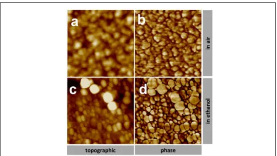
Figure 4 is an example of the so obtained AFM images. The two in the top row have

been taken with the membrane as supplied by the manufacturer in air. The left image (Figure

4.a) displays the topography and the right picture (Figure 4.b) corresponds to the phase

image. The two images in the bottom row were taken after the membrane was drenched in

1 2 3 4 5 6 7 8 9 10 11 12 13 14 15 16 17 18 19 20 21 22 23 24 25 26 27 28 29 30 31 32 33 34 35 36 37 38 39 40 41 42 43 44 45 46 47 48 49 50 51 52 53 54 55 56 57 58

lower quality; for that reason they are not shown here. Images of Figure 4.a and c compare

the topography in both samples. The two images show a granular structure of the polymeric

surface, which is a usual structure for this kind of membranes [48, 49].

In Figure 4.a it is seen that the dried membrane shows less defined granules. This

can be attributed to the presence of preservatives in the membrane and other residues of the

manufacture process. In Figure 4.c, these possible manufacturing conditioning should

probably have been removed and the granules should be enhanced by a swelling effect of

ethanol absorption. A computerized image analysis of the wetted samples shows a granule

size distribution with an average size of 32  12 nm. The granules must correspond to areas

with higher density of polymer. In this sense, it could be presumed that the pores could be

associated to zones of lower polymer density between the granules, or equivalently to the

larger inter granular interstices.

1 2 3 4 5 6 7 8 9 10 11 12 13 14 15 16 17 18 19 20 21 22 23 24 25 26 27 28 29 30 31 32 33 34 35 36 37 38 39 40 41 42 43 44 45 46 47 48 49 50 51 52 53 54 55 56 57 58 59 60 61

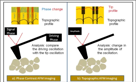
Figure 5.a shows a scheme of the phase change process when the tip moves from

hard to soft areas. Images b and d of Figure 4 show the phase change (in tapping mode)

associated to the change in viscoelastic properties of the surface, providing additional

information to the topographical projections [49].

In the phase contrast images, especially for the wet sample, the polymer granules

and the resulting interstices can be seen with higher definition. This may be associated

(ignoring the possible topographic effect) to lower polymer densities (higher free volume) of

these interstices in support of the probable presence of slit-like pores within these gaps. AFM,

at least directly, is not able to determine pore sizes in membranes having this structure.

From the analysis of our images, we could get slit pore sizes of 6.7  1.8 nm in

thickness and lengths of 42  12 nm. These sizes are bigger than those that would be

expected in a NF membrane. This could be explained because these sizes correspond to the

entrance of the pore formed by the granules that would be narrowed inside the membrane,

and because they were actually observed with a tip larger than the pore. Really, the size

Figure 5: Scheme of AFM analysis of the membrane Surface a) Phase change between hard and soft zones on the Surface b) Topography measure (difference

1 2 3 4 5 6 7 8 9 10 11 12 13 14 15 16 17 18 19 20 21 22 23 24 25 26 27 28 29 30 31 32 33 34 35 36 37 38 39 40 41 42 43 44 45 46 47 48 49 50 51 52 53 54 55 56 57 58

visualized in the image depends on the curvature and the size of the granules and on the tip

geometry. The size observed is always larger than the real size of the pores. Figure 5.b

schematizes the difference between the real profile of the surface and that provided by the tip,

with the consequent increase of the estimated pore size. However, AFM analysis clearly

confirms that the pores of our membrane should have a more slit-like section.

Some more accurate morphological characteristics including the mean pore

radius,r_p, and the active layer thickness,x_a, must be known to be used as inputs for the

model resolution presented above. A mean pore radius of 0.46  0.08nm was obtained

supposing slit pores in retention measurement. In the experimental measurements,

tetraethylene glycol was used, taking concentration polarization into account and following a

procedure exposed elsewhere by us [20] in order to obtain the true retention coefficient and

the corresponding pore-size distribution. This result is close to the 0.48 nm obtained for this

membrane by Hussain et al. [23] using uncharged solute rejection measurements and has

been used in previous works [10, 20, 21]. The validity of the neutral solute retention method

to get information on pore size has been previously tested by us [38]. The thickness of the

active layer, x_a, was measured in our previous work [10] by Environmental Scanning

Electron Microscopy images of transversal sections ( x_a 90 30 nm ).

The transport number of ions inside the membrane was determined from

measurements of membrane potential. Figure 6 shows membrane potential versus the

logarithm of the concentrations ratio. The transport number of the Na+ cation inside the pores

of the active layer, t_1,p, can be determined from the slope of the straight fitted according to

[50]:





memb 1,

low

1 2 _p RTln c

E t

F c

 

  _{ }

1

approximately equal to the concentrations ratio. Calculating the transport number from the

slope of the line implies that it is independent of concentration. This behavior has already

been previously studied for the same membrane and KCl solutions [10].

The value obtained for the cation transport number was t_1,p 0.72 0.03 , which is

bigger than the free solution one: t1,b 0.39 0.01 [51]. This means that there is a clear

increase in the portion of transport carried by cations through the pores. The isoelectric point

for this membrane is less than 3.3, as found in literature [52]. This means that the membrane

is negatively charged when working with these ionic solutions.

The value obtained for water permeability was: 11

w (2.78 0.05)·10 m/s·Pa



 

L .

From Equation (4) and taking b 8.9·10 Pa·s4



 for the bulk viscosity [53], the pore viscosity

p slit

 obtained is (5.4 0.6)·10 Pa·s 3 . And with Equation (3) we can obtain the value of the

porosity- thickness ratio: (4.7 0.8)·10 m 7 . All the membrane properties are summarized in

Table 1.

1

Table1: Modeling fixed parameters.

MEMBRANE PARAMETERS

w

4.2. Impedance Spectroscopy results and modeling

Results obtained with impedance spectroscopy for NaCl solutions for this membrane

were shown previously [21]. The Nyquist’s plot has a very similar behavior to the results

obtained for KCl solutions with the same concentration values [10]. An example of a Nyquist

plot for the studied concentrations is shown in Figure 7. The first lobe, corresponding to high

frequency (low real impedance) represents the solution outside the membrane flowing

through the cell and inside the membrane support where there are no restrictions. The second

lobe (lower frequency) is attributable to the really restrictive part of the membrane; i.e. to the

Z'()

0 500 1000 1500 2000

Z

Figure 7: Nyquist plot for NaCl solution 1mol/m3_{. The best fitting according}

1 2 3 4 5 6 7 8 9 10 11 12 13 14 15 16 17 18 19 20 21 22 23 24 25 26 27 28 29 30 31 32 33 34 35 36 37 38 39 40 41 42 43 44 45 46 47 48 49 50 51 52 53 54 55 56 57 58 59 60 61

pores of the active layer of the membrane. The last lobe, for the lowest frequencies (high real

impedances) corresponds to the relaxation of the polarization layer in contact with the

electrodes and membrane (see Figure 1). The second lobe only appears when the membrane

is present [10], (see supplementary Figure, S-1). It can be seen that the central lobe is where

experimental data best fit the model described by Equation (A.1).

Following the procedure outlined in section 2.1, dielectric parameters of our system

are obtained. In Table 2 the conductance and capacitance of the active layer of the membrane

are shown, for NaCl concentrations studied.

Table 2: Capacities and conductances of the active layer of the membrane.

Concentration (mol/m3)

0.01 0.02 0.1 0.2 1 2 10

 

memb nF

C 990±30 990±30 790±20 700±20 600±18 610±18 610±18

 

memb μS

G 345±10 374±11 513±15 840±30 4590±160 9600±300 49700±1500

4.3. Permittivity and conductivity inside NF pores

The permittivity inside the pores, _p, can be obtained from capacities (table 2) and

Equation (1). In this equation, a value of 3.0 has been assumed for the relative permittivity of

the dry polymer (polyamide), d,[54-55]. In Figure 8.a, the permittivity inside the pores, p,

is plotted against the concentration for slit geometries and also the wet membrane

permittivity is presented, _memb(according Equation (A.8)). The membrane permittivity is

obviously lower than that of the pores. Solid lines in Figure 8.a correspond to the fittings to a

three parameter exponential decay approximation, which was later used for the extrapolation

of_pvalues at higher concentrations.

The dependence of permittivity with membrane thickness is shown by including two

dashed curves representing the variations in _p due to the variations in the estimation of

a

x

1 2 3 4 5 6 7 8 9 10 11 12 13 14 15 16 17 18 19 20 21 22 23 24 25 26 27 28 29 30 31 32 33 34 35 36 37 38 39 40 41 42 43 44 45 46 47 48 49 50 51 52 53 54 55 56 57 58

The results for permittivity inside the pores obtained from the flow and retention

data for NaCl solutions, fitted to the SEDE-VCh model in a previous work [22] is also

included in Figure 8.a versus the concentration, as a dotted line. In this case, the free

parameters in the fit were the permittivity inside the pore and the two Freundlich isotherm

constants. The discrepancy in the permittivity values inside the pores obtained by impedance

spectroscopy and from retention data confirms the possibility that different pairs of values





The p values obtained here for NaCl solutions are very similar to those obtained for

KCl and the same membrane in a previous work [10]. The differences between the two salts

are well within the experimental error. This has also been recently confirmed by other authors

[56] for other membrane and salts. It seems that the changes in _p are due to the confinement

effects and to the concentration more than to the type of salt, at least for simple salts of a 1:1

type.

Figure 8: a) Permittivity inside membrane pores along with the global one for the wet membrane as a function of concentration. The dependence of permittivity on the membrane thickness is also included by showing the ± 30 nm dashed lines. For the wetmembrane, the corresponding lines have

not been drawn to avoid unnecessary complications in the figure. The results for p inside the pores

1 2 3 4 5 6 7 8 9 10 11 12 13 14 15 16 17 18 19 20 21 22 23 24 25 26 27 28 29 30 31 32 33 34 35 36 37 38 39 40 41 42 43 44 45 46 47 48 49 50 51 52 53 54 55 56 57 58 59 60 61

The conductivity inside the pores is calculated with conductance values (table 2) and

Equation (2). We assume that the polymer conductivity is much lower than inside the

solution filled pores [57]. Thus, the second term on the right of Equation (2) can be

neglected. Taking into account Equation (A.10), the conductivity inside the pores is:

a

p memb

ka

x G

A S

  _  _

  (11)

Note, that in this case it is not necessary to know the thickness of the active layer because the

thickness to porosity ratio is obtained directly from the measurements of water permeability

by using Equation (3).

Figure 8.b compares the conductivity into the pores with that of the active layer of

the membrane, which is almost an order of magnitude higher. This value is reasonable taking

into account that the porosity of the active layer, for slit pores, is only 19%. The conductivity

inside the pores is more than three orders of magnitude lower than in free solution (not

presented in Figure 8.b but in the 2.2·10-4 S/m to 1.2·10-1 range. This fact corresponds to an

entirely predictable effect of confinement into the pores reducing ionic mobility.

4.4. Volumetric charge density and ionic mobility inside NF pores

However, in Figure 9 it can be seen, that the ratio of pore to bulk conductivity

varies only slightly, and fits fairly well to Equation (9), for bulk concentrations between 0.01

and 10 mol/m3. Here  x_a 90 nm has been assumed.

For the fitting of Equation (9), the transport number obtained from the membrane

potential measurement has been used. Because the transport numbers are essentially

independent of concentration the ratio of mobilities, _1,p

1,b

U U , should also be almost

1 2 3 4 5 6 7 8 9 10 11 12 13 14 15 16 17 18 19 20 21 22 23 24 25 26 27 28 29 30 31 32 33 34 35 36 37 38 39 40 41 42 43 44 45 46 47 48 49 50 51 52 53 54 55 56 57 58

slit like pores can be fitted to get _1,p

1,b

U U and the parameters of the charge isotherm:  ,  .

Table 3 summarizes the values of the Freundlich isotherm constants (Equation (8)) with the

values of the ratio of mobilities. We note a substantial reduction in ionic mobilities inside the

pore, as reasonable, because the cation confinement inside the pores leads to a considerable

reduction of its mobility.

Table 3: Mobilities ratio and Freundlich isotherm parameters as a function of active layer thickness.

 

a nm

x





1,p 1,b ·10

U U 3





·10 mol m

 

120 10.3 ± 0.2 9.10 ± 0.05 1.02 ± 0.06 90 2.43 ± 0.08 29.3 ± 0.1 0.870 ± 0.009 60 1.48 ± 0.06 30.9 ± 0.1 0.738 ± 0.008

c_b (mol/m3)

10-2 ₁₀-1 ₁₀0 ₁₀1

p b

10-4 10-3

Fitting to eq (9) Experimental data

1

Figure 10 shows the absorbed charge inside the pores of the membrane as a function

of NaCl concentration. The results obtained by using the model proposed by Li and Zhao,

where dielectric effects were not considered [58] are also shown. It is seen that, if these

effects are not taken into account, the model overestimates the membrane charge, because it

has to give the barrier effects on ionic mobilities otherwise contributed by the dielectric

effects.

4.5. SEDE-VCh model predictions

In order to obtain predictions on NaCl rejection, the isotherm presented in Figure 10

and the p correlation in Figure 8.a were used as input of SEDE-VCh model (see appendix B

(Table B.1)). As already mentioned in section 3.3, the rejection experimental values and the

intrinsic rejectionwere taken from a previous work [22]. Both, theoretical and experimental

results, are shown in Figure 11 as a function of the flux of permeate.

In this figure is can be seen that the goodness of the prediction decreases when

concentration increases. There are several reasons for this behavior; firstly, the SEDE-VCh

model should be applied to solutions relatively well diluted, where this assumption is still

Li &Zhao [58] xa=60 nm

xa=90 nm

xa=120 nm

1

heterogeneous adsorption, very commonly used to explain the equilibrium of ionic solutions

with polymer surfaces, although high concentrations could introduce adsorbate-adsorbate

interactions that would be not included within the Freundlich adsorption mechanism [31].

Moreover, _p is extrapolated according to the phenomenological curve (three parameter

exponential decay) fitted to the experimental data (Figure 8.a) that can lose accuracy out of

the range where it was evaluated.

In order to compare the accuracy of the prediction, Figure 12 shows the deviation in

percentage between intrinsic retention values predicted by the model and experimental ones,

as a function of feed concentration, defined as:

int, int,

1

Here R_int,j(exp)is the intrinsic rejection evaluated from the experimental observed retention

for eachJ_{V j,} (exp). R_int,j(cal) is the intrinsic retention predicted by the model and n is the

number of values evaluated for each concentration. It can be seen that the concentration range

where there is not any data extrapolation (concentrations lower than 10 mol/m3, dark shaded

area in Figure 12) the deviations are less than 3%. For extrapolated concentrations, until 50

mol/m3 (light shaded area in Figure 12), deviations are less than 5%, whereas for higher

concentrations, the model underestimates the retention values with higher deviations. As we

have already mentioned, the main cause of this deviation should be the phenomenological

extrapolation of permittivity, conductivity and transport numbers, however other factors such

as the concept of dilute solutions in the model must also influence this discrepancy.

The method used in this study has some difficulty to determine accurately the

permittivity, for concentrations above 10 mol/m3, since the second lobe of the Nyquist plot

(see Figure 7) is too small leading to the necessity of extrapolating over this concentration.

However, recently Efligenir and co-workers [56] designed an experimental method to

determine the permittivity by impedance spectroscopy, isolating the active layer of the

cb(mol/m

Figure 12: Left axis: Deviation in percentage between experimental retention values and intrinsic ones predicted by the model versus the concentration. The line is only an eye guide. Right axis: Product of the inverse Debye length and the

1 2 3 4 5 6 7 8 9 10 11 12 13 14 15 16 17 18 19 20 21 22 23 24 25 26 27 28 29 30 31 32 33 34 35 36 37 38 39 40 41 42 43 44 45 46 47 48 49 50 51 52 53 54 55 56 57 58

membrane. Possibly, this technique could provide values of permittivity at higher

concentrations for NF membranes.

In any case, to predict retention with high and moderately high concentrations, not

only the activity coefficients in Equation (5), should be considered but also the influence of

shielding, which increases with concentration, as pointed out by Dukhin et al. [29].

According to these authors, for membranes with moderately high charge, the simultaneous

dielectric and charge mechanisms produce not simple multiplication of the Donnan and

dielectric factor but a quadratic increase in the intensity of dielectric exclusion. It seems

instructive to plot ratio of the pore radius to the Debye`s lengths, r_p _D, that represent

somehow the charge density. On the right axis of Figure 12 the evolution of r_p _D as a

function of concentration is shown. It can be seen that the region where the deviation between

retentions is higher than 5%, correspond to rp D0.3. If for high values of concentration,

Equation (5) were changed by introducing this quadratic dependence of dielectric exclusion

energy, the retention values calculated would be higher, and probably would approach to the

experimental data.

Of course some aspects of the model itself could be improved. For instance the

parallel pore approximation, used to calculate the dielectric constant inside the pore, that

assumes that the pores are an array of homogeneous equally sized slits, could be improved by

an adequate, but difficult to assess, distribution of pore sizes on the surface and along the

pores themselves. Nevertheless as a consequence of the dielectric behavior of porous walls,

the overall dielectric permeability and conductivity are more trustable than the actual pore

size and thickness values. Other possible source of errors could be due to the assumption of a

independence and separability of the effects of active and support layers that although tested

1 2 3 4 5 6 7 8 9 10 11 12 13 14 15 16 17 18 19 20 21 22 23 24 25 26 27 28 29 30 31 32 33 34 35 36 37 38 39 40 41 42 43 44 45 46 47 48 49 50 51 52 53 54 55 56 57 58 59 60 61

Another quite important expansion of the work presented here could be in the

direction of including multi-ionic salts. Actually, the knowledge of competitive adsorption

isotherms in systems containing several anions remains the main challenge for assessing the

predictive abilities of the methodology proposed, although the transport modeling is

relatively easy to generalize [22]. Of course in such cases impedance spectroscopy and

membrane potential contributions to the methodology studied here have to be modified, and

are being improved, too."

5. Conclusions

From measurements of impedance spectroscopy and applying the model of

interfacial equilibrium we can conclude that: The Impedance Spectroscopy method allows a

separation of the different relaxation processes appearing in a complex membrane system;

although certainly, it is worth taking into account that some aspects of the model could be

still improved as mentioned. Experimental results can be fitted to obtain the conductivity and

permittivity inside the membrane pores, and by modeling, the charge inside the pores. The

confinement of the ions inside the pores reduces both the ionic mobility and the relative

permittivity. The increase in concentration only slightly reduces the value of the permittivity

inside the pores, whereas the ion mobility varies similarly to that of the ions in the free

solution.

Regarding the application of SEDE-VCh model, we can say that, obtaining the

model parameters by independent methods, the model can be used in a predictive way for NF

process. The results are good enough considering the complexity of the mechanisms

involved. The best prediction was found for the diluted concentration according with the

1

method similar to that used by Kita [59] and Asami [60] according to our adaptation [10] and

as

each relaxation time, at low and high frequencies respectively, and G1,lis the conductance of

the system at low frequency. The _i parameters are distribution factors characterizing the

spread of relaxation times [60]. _iis 0, or very near to 0, when the process has a single

relaxation time (Debye type) and the corresponding curve in the Nyquist plot is a perfect

semicircle with its center over the real axis. When the curve presents deviations from a

semicircle, the value of _i is nonzero.

For multilayer systems some constraints in Eq. (A.1) must be fulfilled. These are:

1

parameters and those of the layers was presented by Li and Zhao [58] and confirmed by us

[10]. This description is similar to assuming an equivalent circuit of a number of elements

formed by the combination of a capacitance and a conductance in parallel. In the frequency

range corresponding to the time relaxation of the solution inside the membrane, the phase

parameters can be obtained according to the equations presented in Table A.1. In particular,

permittivity and conductivity in the active layer of the membrane are given by Equations

(A.8) and (A.10) in Table A.1 respectively.

Table A-1. Relation between phase and dielectric parameters [58].

h l

1

In Table B.1 the relationships used within the SEDE-VCh model are shown. These

equations include: transport equations inside the slit shaper pores, partitions at interfaces,

dielectric energies and intrinsic retention, are shown.

Table B.1: SEDE-VCh equations for slit shaped pores.

TRANSPORT EQUATIONS INSIDE PORES





Boundary conditions

a

1 ln 1.19358 0.4285 0.3192 0.08428 1

1 3.02 5.776 12.3675 18.9975 15.2185 4.8525 1

PARTITIONING EQUATIONS







(B.9)

THE DIELECTRIC BORN ENERGY

1

Where a_s is the cavity radius defined by [61] as the distance from the center of the ion to the

point where the relative permittivity becomes different than the vacuum one, ₀.

THE DIELECTRIC IMAGE FORCE ENERGY





and inside the pores respectively.

THE INTRINSIC RETENTION

,perm

8. Acknowledgements

1 2 3 4 5 6 7 8 9 10 11 12 13 14 15 16 17 18 19 20 21 22 23 24 25 26 27 28 29 30 31 32 33 34 35 36 37 38 39 40 41 42 43 44 45 46 47 48 49 50 51 52 53 54 55 56 57 58

References

[1] Y. Lanteri, P. Fievet, A. Szymczyk, Evaluation of the steric, electric, and dielectric

exclusion model on the basis of salt rejection rate and membrane potential

measurements, J. Colloid Interf. Sci., 331 (2009) 148-155.

[2] O. Kedem, A. Katchalsky, Thermodynamic analysis of the permeability of biological

membranes to non-electrolytes, Biochim. Biophys. Acta, 27 (1958) 229-246.

[3] K.S. Spiegler, O. Kedem, Thermodynamics of hyperfiltration (reverse osmosis):

criteria for efficient membranes, Desalination, 1 (1966) 311-326.

[4] J.D. Ferry, Statistical evaluation of sieve constants in ultratiltration, J. Gen. Physiol.,

20 (1936) 95-104.

[5] S.-I. Nakao, S. Kimura, Models of Membrane-Transport Phenomena and Their

Applications for Ultrafiltration Data, J. Chem. Eng. Jpn., 15 (1982) 200-205.

[6] K.H. Meyer, J.F. Sievers, La perméabilité des membranes I. Théorie de la

perméabilité ionique, Helv. Chim. Acta, 19 (1936) 649-664.

[7] T. Teorell, Transport processes and electrical phenomena in ionic membranes, Prog.

Biophys. Biophysical Chem., 3 (1953) 305-369.

[8] X.-L. Wang, T. Tsuru, S.-i. Nakao, S. Kimura, Electrolyte transport through

nanofiltration membranes by the space-charge model and the comparison with

Teorell-Meyer-Sievers model, J. Membr. Sci., 103 (1995) 117-133.

[9] W.R. Bowen, A.W. Mohammad, N. Hilal, Characterisation of nanofiltration

membranes for predictive purposes — use of salts, uncharged solutes and atomic force

microscopy, J. Membr. Sci., 126 (1997) 91-105.

[10] M. Montalvillo, V. Silva, L. Palacio, J.I. Calvo, F.J. Carmona, A. Hernández, P.

Prádanos, Charge and dielectric characterization of nanofiltration membranes by

1 2 3 4 5 6 7 8 9 10 11 12 13 14 15 16 17 18 19 20 21 22 23 24 25 26 27 28 29 30 31 32 33 34 35 36 37 38 39 40 41 42 43 44 45 46 47 48 49 50 51 52 53 54 55 56 57 58 59 60 61

[11] D. Vezzani, S. Bandini, Donnan equilibrium and dielectric exclusion for

characterization of nanofiltration membranes, Desalination, 149 (2002) 477-483.

[12] W.R. Bowen, H. Mukhtar, Characterisation and prediction of separation

performance of nanofiltration membranes, J. Membr. Sci., 112 (1996) 263-274.

[13] W.R. Bowen, A.W. Mohammad, Characterization and Prediction of Nanofiltration

Membrane Performance—A General Assessment, Chem. Eng. Res. Des., 76 (1998)

885-893.

[14] S. Bandini, D. Vezzani, Nanofiltration modeling: the role of dielectric exclusion in

membrane characterization, Chem. Eng. Sci., 58 (2003) 3303-3326.

[15] A. Szymczyk, P. Fievet, Investigating transport properties of nanofiltration

membranes by means of a steric, electric and dielectric exclusion model, J. Membr. Sci.,

252 (2005) 77-88.

[16] S. Déon, A. Escoda, P. Fievet, R. Salut, Prediction of single salt rejection by NF

membranes: An experimental methodology to assess physical parameters from

membrane and streaming potentials, Desalination, 315 (2013) 37-45.

[17] V. Silva, Á. Martín, F. Martínez, J. Malfeito, P. Prádanos, L. Palacio, A.

Hernández, Electrical characterization of NF membranes. A modified model with

charge variation along the pores, Chem. Eng. Sci., 66 (2011) 2898-2911.

[18] C.Y. Tang, Y.-N. Kwon, J.O. Leckie, Effect of membrane chemistry and coating

layer on physiochemical properties of thin film composite polyamide RO and NF

membranes: I. FTIR and XPS characterization of polyamide and coating layer

chemistry, Desalination, 242 (2009) 149-167.

[19] C.Y. Tang, Y.-N. Kwon, J.O. Leckie, Effect of membrane chemistry and coating

1 2 3 4 5 6 7 8 9 10 11 12 13 14 15 16 17 18 19 20 21 22 23 24 25 26 27 28 29 30 31 32 33 34 35 36 37 38 39 40 41 42 43 44 45 46 47 48 49 50 51 52 53 54 55 56 57 58

membranes: II. Membrane physiochemical properties and their dependence on

polyamide and coating layers, Desalination, 242 (2009) 168-182.

[20] N. García-Martín, V. Silva, F.J. Carmona, L. Palacio, A. Hernández, P. Prádanos,

Pore size analysis from retention of neutral solutes through nanofiltration membranes.

The contribution of concentration–polarization, Desalination, 344 (2014) 1-11.

[21] M. Montalvillo, V. Silva, L. Palacio, A. Hernandez, P. Pradanos, Dielectric

properties of electrolyte solutions in polymeric nanofiltration membranes, Desalin.

Water Treat., 27 (2011) 25-30.

[22] V. Silva, V. Geraldes, A.M. Brites Alves, L. Palacio, P. Prádanos, A. Hernández,

Multi-ionic nanofiltration of highly concentrated salt mixtures in the seawater range,

Desalination, 277 (2011) 29-39.

[23] A.A. Hussain, S.K. Nataraj, M.E.E. Abashar, I.S. Al-Mutaz, T.M. Aminabhavi,

Prediction of physical properties of nanofiltration membranes using experiment and

theoretical models, J. Membr. Sci., 310 (2008) 321-336.

[24] S. Van Geluwe, C. Vinckier, L. Braeken, B. Van der Bruggen, Ozone oxidation of

nanofiltration concentrates alleviates membrane fouling in drinking water industry, J.

Membr. Sci., 378 (2011) 128-137.

[25] K. Wesolowska, S. Koter, M. Bodzek, Modelling of nanofiltration in softening

water, Desalination, 163 (2004) 137-151.

[26] W.R. Bowen, J.S. Welfoot, Modelling the performance of membrane

nanofiltration--critical assessment and model development, Chem. Eng. Sci., 57 (2002) 1121-1137.

[27] A.E. Yaroshchuk, Non-steric mechanisms of nanofiltration: superposition of

Donnan and dielectric exclusion, Sep. Purif. Technol., 22-23 (2001) 143-158.

[28] J.N. Israelachvili, Intermolecular and surface forces / Jacob N. Israelachvili,

1 2 3 4 5 6 7 8 9 10 11 12 13 14 15 16 17 18 19 20 21 22 23 24 25 26 27 28 29 30 31 32 33 34 35 36 37 38 39 40 41 42 43 44 45 46 47 48 49 50 51 52 53 54 55 56 57 58 59 60 61

[29] S.S. Dukhin, N.V. Churaev, V.N. Shilov, V.M. Starov, Modelling Reverse Osmosis,

Russ. Chem. Rev., 57 (1988) 572.

[30] A.E. Yaroshchuk, Dielectric exclusion of ions from membranes, Adv. Colloid

Interfac. Sci., 85 (2000) 193-230.

[31] A.W. Adamson, Physical Chemistry of Surfaces, Wiley, New York, 1982.

[32] J.I. Calvo, A. Hernández, P. Prádanos, F. Tejerina, Charge Adsorption and Zeta

Potential in Cyclopore Membranes, J. Colloid Interf. Sci., 181 (1996) 399-412.

[33] L. Dresner, Some remarks on the integration of the extended Nernst-Planck

equations in the hyperfiltration of multicomponent solutions, Desalination, 10 (1972)

27-46.

[34] R. Schlögl, Membrane permeation in systems far from equilibrium, Ber. Bunsen.

Phys. Chem., 70 (1966) 400-414.

[35] T. Tsuru, S.-i. Nakao, S. Kimura, Calculation of Ion Rejection by Extended

Nernst-Planck Equation with Charged Reverse Osmosis Membranes for Single and Mixed

Electrolyte Solutions, J. Chem. Eng. Jpn., 24 (1991) 511-517.

[36] F. Fadaei, V. Hoshyargar, S. Shirazian, S.N. Ashrafizadeh, Mass transfer

simulation of ion separation by nanofiltration considering electrical and dielectrical

effects, Desalination, 284 (2012) 316-323.

[37] Y. Cai, X. Chen, Y. Wang, M. Qiu, Y. Fan, Fabrication of palladium–titania

nanofiltration membranes via a colloidal sol–gel process, Micropor. Mesopor. Mat., 201

(2015) 202-209.

[38] J.A. Otero, O. Mazarrasa, J. Villasante, V. Silva, P. Prádanos, J.I. Calvo, A.

Hernández, Three independent ways to obtain information on pore size distributions of

1 2 3 4 5 6 7 8 9 10 11 12 13 14 15 16 17 18 19 20 21 22 23 24 25 26 27 28 29 30 31 32 33 34 35 36 37 38 39 40 41 42 43 44 45 46 47 48 49 50 51 52 53 54 55 56 57 58

[39] S. Bouranene, P. Fievet, A. Szymczyk, Investigating nanofiltration of multi-ionic

solutions using the steric, electric and dielectric exclusion model, Chem. Eng. Sci., 64

(2009) 3789-3798.

[40] S. Déon, P. Dutournié, P. Bourseau, Modeling nanofiltration with Nernst-Planck

approach and polarization layer, AIChE J., 53 (2007) 1952-1969.

[41] V. Silva, Theoretical foundations and modelling in nanofiltration membrane

systems, in: Física Aplicada, Universidad de Valladolid, Valladolid, 2009, pp. 208.

[42] V.M. Starov, N.V. Churaev, Separation of electrolyte solutions by reverse osmosis,

Adv. Colloid Interfac. Sci., 43 (1993) 145-167.

[43] L. Dresner, Ion exclusion from neutral and slightly charged pores, Desalination, 15

(1974) 39-57.

[44] D. Johnson, N. Hilal, Characterisation and quantification of membrane surface

properties using atomic force microscopy: A comprehensive review, Desalination, 356

(2015) 149-164.

[45] I. Schmitz, M. Schreiner, G. Friedbacher, M. Grasserbauer, Phase imaging as an

extension to tapping mode AFM for the identification of material properties on

humidity-sensitive surfaces, App. Surf. Sci., 115 (1997) 190-198.

[46] L. Martinez, M.A. Gigosos, A. Hernandez, F. Tejerina, Study of some electrokinetic

phenomena in charged microcapillary porous membranes, J. Membr. Sci., 35 (1987)

1-20.

[47] G. Vazquez, E. Alvarez, J.M. Navaza, Surface Tension of Alcohol Water + Water

from 20 to 50 .degree.C, J. Chem. Eng. Data, 40 (1995) 611-614.

[48] D.J. Johnson, S.A. Al Malek, B.A.M. Al-Rashdi, N. Hilal, Atomic force microscopy

of nanofiltration membranes: Effect of imaging mode and environment, J. Membr. Sci.,

1 2 3 4 5 6 7 8 9 10 11 12 13 14 15 16 17 18 19 20 21 22 23 24 25 26 27 28 29 30 31 32 33 34 35 36 37 38 39 40 41 42 43 44 45 46 47 48 49 50 51 52 53 54 55 56 57 58 59 60 61

[49] J. Stawikowska, A.G. Livingston, Assessment of atomic force microscopy for

characterisation of nanofiltration membranes, J. Membr. Sci., 425–426 (2013) 58-70.

[50] N. Lakshminarayanaiah, Transport phenomena in membranes, Academic Press,

New York, 1969.

[51] R.A. Robinson, R.H. Stokes, Electrolyte Solutions: Second Revised Edition, Second

Edition, Revised ed., Dover, London, 2002.

[52] P. Religa, A. Kowalik-Klimczak, P. Gierycz, Study on the behavior of

nanofiltration membranes using for chromium(III) recovery from salt mixture solution,

Desalination, 315 (2013) 115-123.

[53] D.R. Lide, CRC Handbook of Chemistry and Physics, 85 ed., CRC Press, Boca

Raton, FL, 2005.

[54] M.O. Aboelfotoh, C. Feger, Frequency dependence of dielectric loss in thin

aromatic polyimide films, Phys. Rev. B, 47 (1993) 13395-13400.

[55] W.-J. Shang, X.-L. Wang, Y.-X. Yu, Theoretical calculation on the membrane

potential of charged porous membranes in 1-1, 1-2, 2-1 and 2-2 electrolyte solutions, J.

Membr. Sci., 285 (2006) 362-375.

[56] A. Efligenir, P. Fievet, S. Déon, R. Salut, Characterization of the isolated active

layer of a NF membrane by electrochemical impedance spectroscopy, J. Membr. Sci.,

477 (2015) 172-182.

[57] H.-L. Shao, S. Umemoto, T. Kikutani, N. Okui, Electrical Conductivity in Nylon 66

Thin Films Prepared by Alternating Vapor Deposition Polymerization, Polym. J, 31

(1999) 1083-1088.

[58] Y.H. Li, K.S. Zhao, Dielectric analysis of nanofiltration membrane in electrolyte

solutions: influences of electrolyte concentration and species on membrane permeation,

1 2 3 4 5 6 7 8 9 10 11 12 13 14 15 16 17 18 19 20 21 22 23 24 25 26 27 28 29 30 31 32 33 34 35 36 37 38 39 40 41 42 43 44 45 46 47 48 49 50 51 52 53 54 55 56 57 58

[59] Y. Kita, Dielectric-Relaxation in Distributed Dielectric Layers, J. Appl. Phys., 55

(1984) 3747-3755.

[60] K. Asami, Characterization of heterogeneous systems by dielectric spectroscopy,

Prog. Polym. Sci., 27 (2002) 1617-1659.

[61] A.A. Rashin, B. Honig, Reevaluation of the Born model of ion hydration, J. Phys.

Chem., 89 (1985) 5588-5593.

Symbol lists

, , ,

A b B D Parameters defined in Table A.1

k

A Porosity

s

a Cavity radius

C Capacitance

*

C Complex capacitance

c Concentration

d Thickness of the layer in Equation (4)

cell

E Cell potential

memb

E Membrane potential

Nernst

E Solution potential

e Elementary charge

F Faraday constant

f Frequency

G Conductance

1

I Ionic strength

V

J Volumetric flux per unit of membrane area

j Imaginary number 1

,

i c

K Hindrance factor for convection

,

'_{i c}

K Hindrance factor for convection with pressure gradient effect

,

i d

K Hindrance factor for diffusion

B

k Boltzmann constant

L Thickness of layer

w

L Water permeability

N Layer number, pores number or Cl- adsorbed number.

A

N Avogadro’s number

R Universal constant of gases

int

R Intrinsic retention

p

r Pore radius

Stokes

r Stokes radius

S Membrane area

T Temperature

t Transport numbers

U Mobility

x Coordinate