TítuloAn algorithm for the estimation of road traffic space mean speeds from double loop detector data

Texto completo

(1)CIT2016 – XII Congreso de Ingeniería del Transporte València, Universitat Politècnica de València, 2016. DOI: http://dx.doi.org/10.4995/CIT2016.2016.3208 .. 899. An algorithm for the estimation of road traffic space mean speeds from double loop detector data Margarita Martínez-Díaz Assistant Professor, Universidade da Coruña, Spain Ignacio Pérez Pérez Associate Professor, Universidade da Coruña, Spain. ABSTRACT Most algorithms trying to analyze or forecast road traffic rely on many inputs, but in practice, calculations are usually limited by the available data and measurement equipment. Generally, some of these inputs are substituted by raw or even inappropriate estimations, which in some cases come into conflict with the fundamentals of traffic flow theory. This paper refers to one common example of these bad practices. Many traffic management centres depend on the data provided by double loop detectors, which supply, among others, vehicle speeds. The common data treatment is to compute the arithmetic mean of these speeds over different aggregation periods (i.e. the time mean speeds). Time mean speed is not consistent with Edie’s generalized definitions of traffic variables, and therefore it is not the average speed which relates flow to density. This means that current practice begins with an error that can have negative effects in later studies and applications. The algorithm introduced in this paper enables easily the estimation of space mean speeds from the data provided by the loops. It is based on two key hypotheses: stationarity of traffic and log-normal distribution of the individual speeds in each time interval of aggregation. It could also be used in case of transient traffic as a part of any data fusion methodology. 1. INTRODUCTION The evolution of new technologies as well as the efforts of previous researchers have brought us to a powerful situation. Nowadays, practically all kind of traffic studies and projects can be performed by means of a great variety of tools and with quite a deep knowledge of the different phenomena. However, the complexity of many of these analyses and the huge amount of data and calculations required, sometimes lead to the oversight of the fundamentals of traffic flow theory. Thus, erroneous results can be obtained in spite of our current advantageous situation if each step of our studies is not carried out carefully from the very beginning. One common example of malpractice is the use of time mean speeds 𝑣̅𝑡 as equivalent to space mean speeds 𝑣̅𝑠 , although the later are smaller except with space-time homogeneous. This work is licensed under a Creative Commons Attribution-NonCommercial-NoDerivatives 4.0 International License (CC BY-NC-ND 4.0)..

(2) CIT2016 – XII Congreso de Ingeniería del Transporte València, Universitat Politècnica de València, 2016. DOI: http://dx.doi.org/10.4995/CIT2016.2016.3208 .. 900. traffic (Daganzo, 1977). The origin of this misuse is the usual way in which loop detectors, still the main source of data for traffic studies, store the information. Double loops supply vehicle counts n (and classify them according their lengths) and time mean speeds (i.e., the arithmetic mean of the spot speeds) for previously determined time intervals of aggregation. The number of vehicles 𝑛𝑣 𝑎 which pass over the detectors at a speed lower than a particular reference 𝑣 𝑎 is also commonly available. Thus, space mean speeds are not directly provided. They could be obtained from loops if individual spot speeds were stored, as long as they were given certain spatial nature and traffic were stationary in the section (Edie, 1965). They could be then calculated as the harmonic mean of these individual speeds. As in practice only time means are available, some authors have already developed equations that relate both means. The first of them was Equation 1, developed by Wardrop (1952): 𝜎𝑠2. 𝑣̅𝑡 = 𝑣̅𝑠 +. ̅̅̅𝑠 𝑣. (1). where 𝜎𝑠2 is the variance of the speed with respect to the space mean. As this variance is neither available, other equations were postulated. One of them was that of Garber (2002) shown in Equation 2, which was developed experimentally and proved to fail in situations different from that of its estimation. 𝑣̅𝑡 = 0.966𝑣̅𝑠 + 3.541. (2). Equation 3 has been already used in several studies with satisfactory results. It was first derived by Khisty (2003), but proved analytically by Rakha (2005): 𝑣̅𝑠 = 𝑣̅𝑡 −. 𝜎𝑡2 ̅̅̅ 𝑣𝑡. (3). 𝜎𝑡2 is the variance of the speed with respect to the time mean. Although this variance is not directly supplied by the loops, Soriguera and Robusté (2011) developed an algorithm to estimate it. The final expression, shown in Equation 4, involves the assumption of stationary traffic and normality of the speed distribution in each time interval of aggregation. 𝜎𝑡 =. ̅̅̅𝑡 𝑣𝑎− 𝑣. 𝑛𝑣𝑎 𝐹 −1 [ 𝑛 ]. (4). where 𝐹 −1 stands for the inverse of the cumulative normal distribution. Although good results have been obtained in many applications, it seems inappropriate in congestion, specifically in stop and go situations or with shock waves onsets and offsets.. This work is licensed under a Creative Commons Attribution-NonCommercial-NoDerivatives 4.0 International License (CC BY-NC-ND 4.0)..

(3) CIT2016 – XII Congreso de Ingeniería del Transporte València, Universitat Politècnica de València, 2016. DOI: http://dx.doi.org/10.4995/CIT2016.2016.3208 .. 901. 2. ALGORITHM FUNDAMENTALS AND EXPRESSION Keeping in mind the usefulness of Equation 3 in previous studies as well as that of Equation 4 under particular circumstances, the authors of this paper tried to derive another more accurate way of estimating 𝜎𝑡2 . With this aim, and also assuming stationarity of traffic in each time interval of aggregation (supposed short enough to fulfil this assumption), another final formula for the variance with respect to the time mean was obtained (Equation 5): 𝑛𝑎. 𝑣𝑎 2. 𝑛. 𝑣𝑡. 𝜎𝑡2 − 2𝐹 −1 [ 𝑣 ] 𝜎𝑡 + 𝐿𝑛 ( ̅̅̅ ) = 0. (5). The other main assumption behind Equation 5 is that the distribution of the speeds is lognormal (and thus that of the logarithm of the speeds normal), what has allowed the exploitation of its mathematical properties to reach this final equation. And the thing is that, although the normal distribution is the most widely used in this regard because of its simplicity, the log-normal (and also the gamma) distribution is more suitable to represent traffic speeds. It has additional advantages as it avoids the appearance of negative speeds and maintains its shape no matter if time means or their corresponding space means are fitted (Haight, 1962). Even the distribution of travel times derived from speeds that fit the lognormal distribution keeps the same shape (El Faouzi and Maurin, 2007). Some issues must be taken into account when using Equation 5. The first one is that, as it is a quadratic equation, two possible values of 𝜎𝑡 are obtained. And as traffic management centres usually work with two reference speeds (va1 and va2) even four values could be provided. A decision protocol must be thus set up in order to choose the most suitable. One possibility is to keep the value with the smallest confidence interval for a specific level of confidence. Another important fact which is besides related to the former is that, in practice, some values of 𝜎𝑡 are nullified during the calculations because of mathematical limitations mostly related to the cumulative standard normal distribution. As an example, nva must be different from n and from zero to prevent the inverse of this distribution from tending to infinite. Obviously, the proposed methodology is based on the availability of nva. It would not be worth carrying out modifications in the controllers of the management centres to store it, as it would be simpler and more profitable in this case to make the necessary changes to directly obtain space means from the loops. Nevertheless, this parameter is often available, at least with one reference value of speed.. This work is licensed under a Creative Commons Attribution-NonCommercial-NoDerivatives 4.0 International License (CC BY-NC-ND 4.0)..

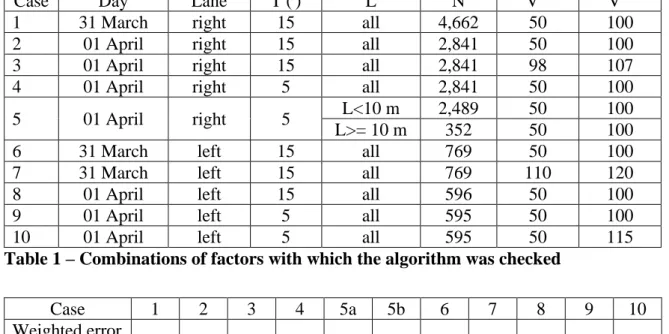
(4) 902. CIT2016 – XII Congreso de Ingeniería del Transporte València, Universitat Politècnica de València, 2016. DOI: http://dx.doi.org/10.4995/CIT2016.2016.3208 .. 3. APPLICATION OF THE ALGORITHM WITH IDEAL AND REAL DATA Some tests were performed in order to verify the goodness of the algorithm. Firstly, it was checked with artificial ideal data generated with Matlab. Secondly, it was tested under different conditions with real data. 3.1 Application with ideal data As mentioned, data that ideally fulfilled the main hypotheses of the algorithm, i.e., stationarity of traffic and log-normality of the speeds in each time interval of aggregation, were mathematically generated to test it. As expected, the space mean speeds estimated by the algorithm were much closer to the “real” space means (obtained in this case as harmonic means of individual speeds) than the time mean speeds. The error that could be introduced by the later in subsequent calculations would be of the order of 2.17%, opposite to the 0.65% of the estimated space means. 3.2 Application with real data Real data were specially collected for this research on March 31th and April 1st, 2014 in a two-lane section (P.K. 86+211 in the direction to A Coruña) with double loops of the AP-9 freeway, which runs north and south along the west coast of Galicia, in Spain. Among others, individual speeds as well as counts n, time means 𝑣̅𝑡 and number of vehicles nva with speeds lower that two of reference (by default va1=50 and va2=100 Km/h) for time intervals of aggregation of T=15 minutes were supplied. All of them per lane. The fact of counting with individual data allowed the authors to check the algorithm under different boundary conditions (e.g. on different days, in different lanes, taking into account all the vehicles or only those with a particular size, setting different reference speeds, etc.). N is the total number of concerned vehicles in each case. Table 1 includes a summary of all the cases that were analyzed and Table 2 makes a comparison of the errors introduced by the algorithm and those usually committed with the use of time means. The implementation of the algorithm was worth doing in eight out of the eleven cases analyzed. However, in cases 6 and 8 the methodology failed. This point is discussed in section 4. It must be also taken into account that the validity of the algorithm must be decided by focusing on the different combinations of variables and not only on any of them. For example, between cases 6 (where the algorithm failed) and 7 (where it improved the results obtained by the current procedure, i.e., by the use of time means as equivalent to space means), only one variable was different, in this case the reference speeds. This and other considerations are also faced in the next section 4.. This work is licensed under a Creative Commons Attribution-NonCommercial-NoDerivatives 4.0 International License (CC BY-NC-ND 4.0)..

(5) CIT2016 – XII Congreso de Ingeniería del Transporte València, Universitat Politècnica de València, 2016. DOI: http://dx.doi.org/10.4995/CIT2016.2016.3208 .. 903. L N Va1 all 4,662 50 all 2,841 50 all 2,841 98 all 2,841 50 L<10 m 2,489 50 5 01 April right 5 L>= 10 m 352 50 6 31 March left 15 all 769 50 7 31 March left 15 all 769 110 8 01 April left 15 all 596 50 9 01 April left 5 all 595 50 10 01 April left 5 all 595 50 Table 1 – Combinations of factors with which the algorithm was checked Case 1 2 3 4. Day 31 March 01 April 01 April 01 April. Lane right right right right. T (') 15 15 15 5. Va2 100 100 107 100 100 100 100 120 100 100 115. Case 1 2 3 4 5a 5b 6 7 8 9 10 Weighted error 1.35 1.19 1.21 2.04 1.68 0.27 0.56 0.47 0.59 1.48 0.93 with time means (%) Weighted error 0.79 0.87 0.99 0.59 0.46 0.86 0.44 0.78 0.58 0.50 with the algorithm (%) Table 2 – Comparison of the errors obtained with the current procedure and that obtained with the algorithm 4. DISCUSSION A deep sensibility analysis was performed in order to check which factors made the algorithm more prone to obtain accurate results. Specifically, the influence of the sample size, the fitting of the speeds to the log-normal distribution, the length of the time interval of aggregation, the type of vehicles, the general traffic conditions, the reference speeds as well as the place, day and moment of data acquisition were tested. As mentioned, most of these factors have been actually considered simultaneously. The key results of this sensibility analysis are briefly explained in the following paragraphs. The first two factors are in fact closely related. As log-normality of speeds in each time interval of aggregation is one of the fundamental hypotheses of the methodology, it must obviously hold. Many studies have demonstrated at this respect that the larger the sample size, the bigger the probability of having this distribution. Traffic conditions and the prevailing type of vehicles have also a relationship with this probability. With low densities, the speeds of light and heavy vehicles can be very different and therefore the algorithm must be used with data of single lanes. If it were used with data of whole sections, bimodal or even multimodal distributions of speed were more probable and thus the methodology would fail. Nevertheless, with medium-high densities, log-normal distributions are possible even with different kinds of vehicles (in these situations their singular behaviour is limited by traffic conditions) and the algorithm could perform well even at a cross-sectional level.. This work is licensed under a Creative Commons Attribution-NonCommercial-NoDerivatives 4.0 International License (CC BY-NC-ND 4.0)..

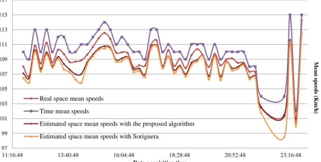
(6) CIT2016 – XII Congreso de Ingeniería del Transporte València, Universitat Politècnica de València, 2016. DOI: http://dx.doi.org/10.4995/CIT2016.2016.3208 .. 904. A trade-off decision must be made with regard to the length of the time interval of aggregation. On the one hand and as explained, it should be quite long so as to include a big number of vehicles. But on the other hand, the other main hypothesis of the methodology, i.e. the stationarity of traffic in each time interval of aggregation, would be jeopardized, as the longer the interval, the easier the appearance of transients. The final length should be then decided once analysed the general traffic conditions. The selection of the reference speeds, if possible, should be made only with a practical purpose, i.e. to have big samples for the analyses. For example in the particular situation of this study, the reference speed of 50 Km/h was useless, as there were only a few vehicles that travelled with speeds lower than this on the freeway. Values between the 90 and the 98% of the average speeds have been proved to be suitable. As for the place, day and moment of the analysis, it is clear that they are related to all the mentioned factors, taking into account that the different average traffic conditions that can exist rely highly on them. The previous considerations show the goodness of the algorithm in most cases. Nevertheless, it must be recognised that it is a bit more complicated than that proposed by Soriguera and Robusté (2011). A final analysis was made at this respect, in which the results of the application of both algorithms were compared. As shown in the example of Figure 1 (where time means and real space means are also sketched), the log-normal algorithm achieves better results. Specifically for the case of the figure (case 1), the weighted mean error of the normal-algorithm would be of 1.05% opposite to the 0.79% of the proposed methodology. 117 115 113 111 Mean speeds (Km/h). 109 107 105 103. Real space mean speeds Time mean speeds. 101 99 97 11:16:48. Estimated space mean speeds with the proposed algorithm Estimated space mean speeds with Soriguera 13:40:48. 16:04:48 18:28:48 Data acquisition time. 20:52:48. 23:16:48. Fig. 1 – Comparison of the results obtained in case 1 with the proposed algorithm and the algorithm of Soriguera and Robusté (2011).. This work is licensed under a Creative Commons Attribution-NonCommercial-NoDerivatives 4.0 International License (CC BY-NC-ND 4.0)..

(7) CIT2016 – XII Congreso de Ingeniería del Transporte València, Universitat Politècnica de València, 2016. DOI: http://dx.doi.org/10.4995/CIT2016.2016.3208 .. 905. 5. CONCLUSIONS AND FUTURE RESEARCH The control of traffic evolution has experimented a great improvement in the last years thanks to the efforts of researchers and the appearance of new tools for data collection and analysis. However, the fundamentals of traffic flow theory should not be forgotten among complicated formulas if we aim at achieving accurate results. One example of these fundamentals is the use of the correct mean speed when using this factor for any subsequent purpose. In most cases, and as they relate flows to densities, space mean speeds are needed. However, traffic management centres primarily work with time means, which are erroneously considered equivalent to space means. This paper introduces an algorithm to estimate the later from the former in each time interval of aggregation, without the need for extra expenses. A complete analysis with different boundary conditions was performed and the following conclusions have been drawn: . . . . it is possible to improve the current procedure followed by most traffic management centres, i.e., the indiscriminate use of time mean speeds as substitutes of space means, even with the same equipment usually available, which mostly consists on double loop detectors. The procedure introduced in this paper is a clear example, which worked well in most of the cases analysed. the main hyphoteses of the algorithm must hold to achieve accurate results. Therefore, traffic must be stationary and there must exist a log-normal distribution of speeds in each time interval of aggregation. A good design of the conditions of data acquisition (and thus of the implementation of the algorithm) can often help to fulfil these requirements. as a summary, accurate results are usually achieved when working per lane, with medium-short time intervals of aggregation and with reference speeds between the 90 and 98% of the average speed of the freeway. the algorithm is not accurate in case of transients, stop and go situations, etc. But even in these cases, it could be very profitable when used together with information from other sources, within a data fusion procedure.. Additionally, further research could reinforce the utility of the proposed algorithm. Examples of possible future lines are:  . . the design of a process to smooth or correct the tendency of the loops to drift, as they are the main source of data. the inclusion in the algorithm of the necessary steps to calculate the confidence interval for the estimated space means for those cases where more than one result is obtained from the calculations. the development of similar algorithms for the case of the existence of gamma or even. This work is licensed under a Creative Commons Attribution-NonCommercial-NoDerivatives 4.0 International License (CC BY-NC-ND 4.0)..

(8) CIT2016 – XII Congreso de Ingeniería del Transporte València, Universitat Politècnica de València, 2016. DOI: http://dx.doi.org/10.4995/CIT2016.2016.3208 .. 906. . multimodal distributions of speeds. Along with another one to previously detect the distribution that exists, the most suitable algorithm for the calculation of the space means could be assigned in each case. the development of data fusion schemes that include the proposed algorithm, e.g. in combination with information provided by new tools such as Bluetooth or GPS.. As it has been already remarked, in spite of the improvement that traffic analysis has experimented in the last years, there is still a lot of research to do, specially for the case of non-stationary traffic (existence of shock waves, stop and go situations, etc.). The simultaneous use of different sources of information and analysis seems promising, as long as the basic principles of traffic flow are not broken. 6. ACKNOWLEDGMENTS This research would not have been possible without the support of the Centro de Gestión del Tráfico del Noroeste (Dirección General de Tráfico, Government of Spain), in particular of its Manager, Mr. Ramiro Martínez Rodríguez, who supplied us the data used for the study. 7. REFERENCES DAGANZO, C. (1997). Fundamentals of Transportation and Traffic Operations. Pergamon, Oxford. ISBN: 0080427855. EDIE, L. (1965). Discussion of traffic stream measurements and definitions. Proceedings 2nd International Symposium on the Theory of Traffic Flow. OECD, París, pp. 139-154. EL FAOUZI, N. and MAURIN, M. (2007). Reliability of travel time under log-normal distribution: methodological issues and path travel time confidence derivation. Transportation Research Board 86th Annual Meeting (CD- ROM). Transportation Research Record, Washington D.C. GARBER, N. H. (2002). Traffic and Highway Engineering. Brooks/cole, California. ISBN 0-534-38743-8. HAIGHT, F. M. (1962). A practical method for improving the accuracy of vehicular vehicle speeds distribution measurements. Highway Research Board Bulletin 341, pp. 92-116. KHISTY, C. L. (2003). Transportation Engineering: An Introduction. Prentice Hall, New Jersey. ISBN 0-13-033560-6. RAKHA, H. Z. (2005). Estimating traffic stream space-mean speed and reliability from dual and single loop detectors. Transportation Research Record: Journal of de Transportation Research Board 1925, pp. 38-47. DOI: 10.3141/1925-05. SORIGUERA, F. and ROBUSTÉ, F. (2011). Highway travel time accurate measurement and short-term prediction using multiple data sources. Transportmetrica 7(1), pp. 85-109. DOI:10.1080/18128600903244651. WARDROP, J. (1952). Some theoretical aspects of road traffic research. Proceedings of the Institute of Civil Engineers 1(2), pp. 325-378. DOI: 10.1680/ipeds.1952.11259.. This work is licensed under a Creative Commons Attribution-NonCommercial-NoDerivatives 4.0 International License (CC BY-NC-ND 4.0)..

(9) CIT2016 – XII Congreso de Ingeniería del Transporte València, Universitat Politècnica de València, 2016. DOI: http://dx.doi.org/10.4995/CIT2016.2016.4093 .. 907. EXPERIMENTS SIMULATION AND DESIGN TO SET TRAFFIC LIGHTS’ OPERATION RULES Jaime Espinoza Mondragón Master Student, Instituto Tecnológico de Celaya, México José Alfredo Jiménez García, José Martin Medina Flores and José Antonio Vázquez López Research Professor, Instituto Tecnológico de Celaya, México Sandra Téllez Vázquez Research Professor, Universidad Politécnica de Guanajuato, México ABSTRACT In this paper it is used the experimental design to minimize the travel time of motor vehicles, in one of the most important avenues of Celaya City in Guanajuato, Mexico, by means of optimal synchronization of existing traffic lights. In the optimization process three factors are considered: the traffic lights’ cycle times, the synchrony defined as stepped, parallel and actual, and speed limit, each one with 3 evaluation levels. The response variables to consider are: motor vehicles’ travel time, fuel consumption and greenhouse effect gas (CO2) emissions. The different experiments are performed using the simulation model developed in the PTV-VISSIM software, which represents the vehicle traffic system. The obtained results for the different proposed scenarios allow to find proper levels at which the vehicle traffic system must be operated in order to improve mobility, to reduce contamination rates and decrease the fuel consumption for the different motor vehicles that use the avenue. 1. INTRODUCTION In the city of Celaya, Guanajuato there are released every year 873,111 tons of CO2 (Aranda García et al., 2013), this due the increasing demand of vehicles that use these routes in the city. It is worth to mention that Blvd. Adolfo López Mateos (Blvd. ALM ) is one of the busiest routes and for this reason it is worth to reduce travel time of any vehicle that use this road system. Exhaust emissions from motor vehicles contain more than 100 kinds of harmful substances, including the main component of particulate matter, carbon dioxide (CO2), carbon monoxide (CO), nitrogen oxide (NOX) and hydrocarbons (HC) etc. (Zhipeng, Lizhu, Shanqzhi, & Yeqing Qian, 2014). The severity of the problem rises when the traffic flow is interrupted and the delays and start–stops occur frequently. These phenomena are regularly observed at traffic intersections, junctions, and at signalized roadways (Pandian, Gokhale, & Goshal, 2009). During idle period, the engine will consume more fuel and will release more CO2 emissions than in travel time (M. Barth & K. Boriboonsomsin, 2009). Although a study. This work is licensed under a Creative Commons Attribution-NonCommercial-NoDerivatives 4.0 International License (CC BY-NC-ND 4.0)..

(10)