Complex dynamics of photonic delay systems: a story of consistency and unpredictability

Texto completo

(1)DOCTORAL THESIS 2015 COMPLEX DYNAMICS IN PHOTONIC DELAY SYSTEMS: A STORY OF CONSISTENCY AND UNPREDICTABILITY. Neus Oliver Andreu.

(2) DOCTORAL THESIS 2015 Doctoral Program of Physics. COMPLEX DYNAMICS OF PHOTONIC DELAY SYSTEMS: A STORY OF CONSISTENCY AND UNPREDICTABILITY. Neus Oliver Andreu Thesis Supervisor: Ingo Fischer Tutor: Claudio R. Mirasso Doctor by the Universitat de les Illes Balears.

(3) ii Complex dynamics in photonic delay systems: a story of consistency and unpredictability Neus Oliver Andreu Tesis presentada en el Departamento de Fı́sica de la Universitat de les Illes Balears. PhD Thesis Director: Dr. Ingo Fischer.

(4) iii. El Profesor Ingo Fischer, Profesor de Investigación del Consejo Superior de Investigaciones Cientı́ficas (CSIC) y el Profesor Claudio Mirasso, Catedrático de Universidad (UIB), HACEN CONSTAR que esta tesis doctoral ha sido realizada por la Sra. Neus Oliver Andreu bajo su dirección en el Instituto de Fı́sica Interdisciplinar y Sistemes Complejos (UIB-CSIC) y, para dejar constancia, firma la misma. Palma, 12 de noviembre de 2015. Ingo Fischer Director. Claudio Mirasso Ponente. Neus Oliver Andreu Doctorando.

(5) iv.

(6) When you come out of the storm you won’t be the same person that walked in. That’s what the storm is all about. - Haruki Murakami.. v.

(7)

(8) Resumen El campo de la fotónica está revolucionado nuestra industria y sociedad actuales. Sus usos no se limitan a ciencia avanzada y muchas de sus aplicaciones están integradas en nuestra vida diaria: internet depende de las comunicaciones ópticas por fibra, los láseres son una herramienta más en cirujı́a médica y fabricación industrial, y el uso de la luz ha facilitado el desarrollo de técnicas de metrologı́a, entre otros. La fenomenologı́a en fotónica hace de ella un campo lleno de posibilidades y potencial por explorar. Dos de las áreas más prometedoras son el procesamiento de información y comunicaciones ópticas seguras. Contribuyendo a dichas áreas, esta tesis estudia el comportamiento complejo y emergente en un sistema fotónico concreto: el láser de semiconductor con retroalimentación. Este sencillo sistema es capaz de generar gran variedad de regı́menes dinámicos, como caos determinista. Con él, abarcamos las propiedades de consistencia para el procesamiento de la información, y la generación de números aleatorios, escribiendo una historia de consistencia e impredecibilidad. Sobre consistencia o cómo procesar información por medios fotónicos Nuestro cerebro es un órgano eficiente, capaz de realizar de manera fiable tareas complicadas como el reconocimiento de caras. Inspirándose en el cerebro, se han desarrollado nuevos métodos para imitar el procesamiento de la información en redes neuronales, entre ellos ”Reservoir Computing”. En esta técnica, un sistema fotónico no lineal es capaz de efectuar tareas computacionalmente arduas al proporcionar respuestas consistentes a señales de entrada. La capacidad de un sistema de responder de manera similar a estı́mulos similares, o consistencia, es una cualidad natural que, sorprendentemente, no está asegurada. Su cuantificación y mecanismos causantes son temas por investigar y los láseres de semiconductor con retroalimentación representan una plataforma excelente para ello. Por medio de tres experimentos investigamos, caracterizamos y cuantificamos las propiedades de consistencia en esquemas ópticos y optoelectrónicos. Los experimentos ilustran transiciones entre respuestas consistentes e inconsistentes, ası́ como su dependencia con respecto al tipo y naturaleza de la señal de entrada. Más allá del mundo de la fotónica, la consistencia es un concepto relevante en ciencia y tecnologı́a. Las propiedades y métodos desarrollados en esta tesis representan un avance para futuras investigaciones y aplicaciones. vii.

(9) viii Sobre impredecibilidad o cómo implementar un generador de números aleatorios óptico Los números (bits) aleatorios, son cruciales para transmisión de información segura, juegos online, simulaciones numéricas o criptografı́a. Su ubicuidad ha provocado la aparición de generadores de números aleatorios (RNGs) basados en componentes fotónicos con claras ventajas: pueden integrarse fácilmente en sistemas de telecomunicaciones actuales y permiten la generación a velocidades altas (Gbit/s). Aunque se han implementado algunos RNGs ópticos exitósamente, quedan cuestiones por resolver: ¿Es posible emplear esquemas más sencillos para generar números aleatorios? ¿Estamos empleando los RNGs de manera óptima? ¿Cuál es el ritmo máximo de generación posible? ¿Podemos conocerlo de antemano? Esta tesis contribuye a responderlas. Proponemos un experimento simple basado en un láser de semiconductor con retroalimentación, aprovechando la impredecibilidad de su dinámica caótica. Sin embargo, la dinámica es condición necesaria pero no suficiente para obtener números aleatorios. En la comprensión de los factores determinantes en la generación de números aleatorios y las altas velocidades de generación reside la relevancia de este trabajo..

(10) Summary The field of photonics is revolutionizing the current industry and society, analogously to what electronics did during the 20th century. The uses of photonics seem endless and are not restricted to advanced science. Some of its applications have already become mature technologies, and belong now to our everyday life: internet relies on optical fiber communications, lasers are an integrated tool in medical surgery and industrial manufacturing, and the use of light has facilitated the measurement techniques in metrology, among many others. The rich phenomenology in photonics makes it an emerging field with open perspectives, whose full capabilities are still to be exploited. Specifically, two of the promising areas for photonics are information processing and secure optical communications. Complex phenomena in photonics can serve as a backbone for both applications. This Thesis comprises the study of the emerging complex behavior in a concrete photonic system: a semiconductor laser with delayed feedback. This simple system can generate an interesting variety of dynamical regimes, like deterministic chaos and, therefore, we use it to contribute to the above mentioned areas. More precisely, we address the consistency properties for bio-inspired photonic information processing and the optical generation of random numbers, thereby telling a story of consistency and unpredictability. On consistency or how to perform reliably photonic information processing Our brain is a fast and efficient organ, capable of performing reliably tasks that for any computer would be rather hard, such as face recognition. Inspired by our brain, technical systems have been introduced to mimic information processing in neural networks. Understanding how these systems process information can lead to faster, low-energy demanding computing. A recent technique for photonic information processing is Reservoir Computing. In Reservoir Computing, a nonlinear system performs computationally hard tasks, like spoken digit recognition. Its operation is based on providing a consistent nonlinear response with respect to an input signal, exactly as neurons do: they respond reliably to electrical and chemical signals when processing information. Consistency, as the ability of the system to respond in a similar way to similar inputs, is therefore a key-ingredient to be studied. Surprisingly, consistency in nature is not always a given, and a system might change from a consistent response to an inconsistent one. The mechanisms underlying consistency as well as its quantification are thus pertinent proper questions. Semiconductor lasers with feedback represent again an excellent platform for its investigation. ix.

(11) x We approach these aspects by designing three experiments to investigate and characterize the consistency properties of semiconductor laser with delayed optical and opto-electronic feedback. The high quality of the experiments allow us to illustrate the occurrence of transitions between consistent and inconsistent responses in the laser, and characterize their dependence on the drive signal. Thus, we utilize various drive signals, both optical and electrical, and present different ways to quantify consistency, including correlations and a direct measure for the sub-Lyapunov exponent. Beyond photonics, consistency in driven systems is a fundamental and far-reaching concept, present in nature and technology. Therefore, the fundamental properties and the developed method represent valuable findings for further fundamental investigations and applications. On unpredictability or how to implement an optical random number generator Random numbers (or random bits) are crucial for information security, online-gaming, complex numerical simulations and cryptography. Their ubiquity has led to the emergence of random number generators (RNGs) based on photonic components, given the intrinsic advantages of photonics: first, an optical RNG is easy to integrate into telecommunication systems; and second, a photonic approach to random number generation allows for high generation speeds of order of gigabits per second (Gbit/s), a key demand of current random number generators. Although some optical approaches to random bit generation had been successfully put forward, open questions still remained: Is it possible to employ simpler schemes to generate random numbers? Are we using the RNG optimally or can its performance be enhanced? What is the maximum bit rate attainable with a given RNG? Can we know it in advance? In this Thesis, we contribute significantly to answer these questions. We propose a strikingly simple experimental setup based on a single semiconductor laser with optical feedback, benefiting from the unpredictability and randomness of the chaotic output of the laser. Nevertheless, chaotic dynamics is only a necessary but not a sufficient condition to obtain random numbers. We present guidelines on the interplay between dynamics, acquisition procedures and post-processing, and predict the potential of any RNG by using Information Theory to estimate the maximum achievable bit rate. The relevance of this work relies not only on the high speed of the bit rate, up to 160Gbit/s, but also on the understanding of the factors involved in the random bit generation process to guarantee the optimal operation of any laser-based generator..

(12) Acknowledgements If someone had told me ten years ago that I would be writing these lines today, I wouldn’t had believed them. At that time I was convinced that Physics was cool, but not for me. And here I am with a PhD Thesis that has my name on it. Certainly, I could not have done this work without the help and contribution of so many people throughout these years. I would like to express my deep gratitude to Prof. Ingo Fischer. His patience, support, respect, perseverance, passion towards science and motivation were the constant attributes of his wise guidance. Discussions with him were always a source of inspiration, and despite my atelophobia, he kept encouraging me every time I felt hopeless. From him, I learnt that failure is only part of success and that giving up is never a choice. I feel very lucky to have had as an advisor a person I admire so much, as a scientist and as a human being. I cannot forget the person responsible of my first steps into research and the first to believe I was capable of pursuing a PhD: Prof. Maxi San Miguel. Thanks for trusting in me. I am also very grateful to Prof. Claudio Mirasso for his advice and for being so supportive and caring during these years. With the doors of his office wide open at any time, he always had encouraging words for me and I can never thank him enough for his kindheartedness. I would also like to thank all the collaborators and colleagues that I got to meet and from whom I learnt so much: Dr. Miguel C. Soriano for guiding me into the world of experimental photonics, Dr. David Sukow for his kindness, constant support and pleasant emails, Dr. FanYi Lin for his hospitality when I did the research training in Taiwan and Dr. Laurent Larger for welcoming me in his labs and introducing me to the optoelectronic oscillator. I also thank Dr. Daniel Brunner for his willingness to help at any time and always with a smile on his face. I also want to give credit to Dr. Thomas Jüngling. His mentoring, excellent work and, above all, friendship, have meant a lot to me. I also want to thank Dr. Jordi Garcı́a-Ojalvo, Antonio Pons, Javier Buldú, Maria del Carme Torrent and Jordi Tiana-Alsina. I am also grateful to each and every person at IFISC, for the inspiring atmosphere they create and the good memories that I will take with me. I am particularly thankful to all the members of the Nonlinear Photonics Lab, specially to my dudes Xavier Porte and Konstantin Hicke. I also want to thank Dr. Pere Colet and Dr. Roberta Zambrini for the nice interactions along these years, and all the current and former students at the S07. I want to express my gratitude to the technical and administrative staff: Marta Ozonas, Inma Carbonell, Rosa Marı́a Rodrı́guez, Rosa Campomar, Rubén Tolosa, Edu Herraiz, Antònia Tugores, Pep Canyelles, Daniel Palou and Edu Solivellas. As a PhD student I got to meet a lot of amazing colleagues from around the globe. I xi.

(13) xii am thankful to all the nice people at the National Tsing Hua University in Taiwan, specially Chih-Hao Cheng, Jack Wu and Yi-Huan Liao. To all the scientists I met at FEMTO-ST, particularly to Jacques Chrétien, Bicky A. Márquez, Guoping Lin, Shanti Toenger, Antonio Baylon, Xavier Romain, Tintu Kuriakose, Bogdan Penkovsky and Ignacio Zaldivar. I would also like to mention Dr. Anbang Wang, Dr. Yun-cai Wang and Dr. Alan Shore for the nice time in China. The best thing about this time as PhD student is to have had colleagues that ended up being real friends. I am happy to have shared so many good times with Marina Diakonova, Antònia Tugores and Thomas Jüngling. Thank you for being by my side and for accepting my craziness with no judgements. I look forward to our next adventures together. I am also deeply grateful to Valérie Moliere, for her tremendous support in my joys and struggles. To my friend Tawnee Hensel, because even though we don’t see each other as much as we would like to, we still can count on each other. Last but not least, I want to thank my parents and my brother. Aunque no seamos la familia más convencional, soy muy feliz de teneros a mi lado. Gracias por apoyarme aún sin saber muy bien qué he estado haciendo. And above all, I want to thank Toni Buades, for being a partner, a friend and a fellow traveler; for his patience, limitless understanding, and for embracing the mess that I am. Thanks for sharing your life with me..

(14) List of Publications • Neus Oliver, Miguel C. Soriano, David W. Sukow and Ingo Fischer. Dynamics of a semiconductor laser with polarization-rotated feedback and its utilization for random bit generation. Optics Letters, 36, 23, 4632, (2011). • Neus Oliver, Miguel C. Soriano, David W. Sukow and Ingo Fischer. Fast random bit generation using a chaotic laser: approaching the information theoretic limit. Journal of Quantum Electronics, 49, 11, 910, (2013). • Neus Oliver, Thomas Jüngling and Ingo Fischer. Consistency properties of a chaotic semiconductor laser driven by optical feedback. Physical Review Letters, 114, 12, 123902, (2015). Manuscripts in preparation • Neus Oliver, Javier M. Buldú, Antonio J. Pons, Jordi Tiana-Alsina, M. Carme Torrent, Ingo Fischer and Jordi Garcı́a-Ojalvo. Consistency through transient dynamics. To be submitted, PNAS. • Neus Oliver, Bicky A. Márquez, Laurent Larger and Ingo Fischer Forms of consistency in a multistable driven system: the Ikeda oscillator case. Conference contributions • M. C. Soriano, N. Oliver, X. Porte, R. Vicente, I. Fischer and C. R. Mirasso. Delay Coupled Semiconductor Lasers: Dynamics and Applications. VII Reunin Iberoamericana de ptica (RIAO). X Encuentro Latinoamericano de ptica, Lseres y Aplicaciones (OPTILAS), Lima, Peru, 2010. Invited Talk. • N. Oliver, M. C. Soriano, D. W. Sukow and I. Fischer. Dynamics of semiconductor lasers with polarization rotated feedback and its applications for fast random bit generation. European Conference on Lasers and ElectroOptics (CLEO Europe) and the XIIth European Quantum Electronics Conference, Munich, Germany, 2011. Talk. • N. Oliver, M. C. Soriano, D. W. Sukow and I. Fischer. Dynamics of semiconductor lasers with delayed polarization rotated feedback and its applications for fast random bit generation. Combined DPG Spring Meeting, Berlin, Germany, 2012. Talk. xiii.

(15) xiv • N. Oliver, M. C. Soriano, D. W. Sukow and I. Fischer. Dynamics of semiconductor lasers with delayed feedback and its applications for fast random bit generation. International Conference on Delayed Complex Systems (DCS12), Palma de Mallorca, Spain, 2012. Poster. • N. Oliver, M. C. Soriano, D. W. Sukow and I. Fischer. Experimental Criteria for highspeed random bit generation using a chaotic semiconductor laser. European Conference on Lasers and Electro-Optics (CLEO Europe) and the XIIIth European Quantum Electronics Conference, Munich, Germany, 2013. Talk. • N. Oliver and I. Fischer. Exploring chaotic semiconductor lasers for high speed random bit generation: practical and information theoretic limitations. The 6th International Workshop on Chaos Fractals Theories and Applications, Shanxi, China, 2013. Invited Keynote. • N. Oliver, T. Jüngling, D. Brunner, A. J. Pons, J. Tiana-Alsina, J. Buldú, M. C. Torrent, J. Garcı́a-Ojalvo and I. Fischer. Consistency Properties of a Chaotic Laser to Input Pulse Trains. European Conference on Lasers and Electro-Optics and the European Quantum Electronics Conference, Munich, Germany, 2015. Poster..

(16) Contents Resumen. vii. Summary. ix. Acknowledgements. xi. List of Publications. xiii. 1 Introduction 1.1 Delay systems . . . . . . . . . . . . . . . . . . . . . . . . . . 1.2 Photonic delay systems . . . . . . . . . . . . . . . . . . . . 1.2.1 Photonic delay systems in the drive-response scheme 1.3 About Consistency . . . . . . . . . . . . . . . . . . . . . . . 1.3.1 Applications of consistency . . . . . . . . . . . . . . 1.4 About Unpredictability . . . . . . . . . . . . . . . . . . . . 1.4.1 Applications of unpredictable dynamics . . . . . . . 1.5 Overview of this Thesis . . . . . . . . . . . . . . . . . . . . 2 Concepts and tools 2.1 Consistency and Generalized Synchronization 2.2 Tools to measure consistency . . . . . . . . . 2.2.1 The sub-Lyapunov exponent . . . . . 2.2.2 Inter- and intra-correlations . . . . . . 2.2.3 Review of the consistency measures . 2.3 Tools to measure unpredictability . . . . . . .. . . . . . . . .. . . . . . . . .. . . . . . . . .. . . . . . . . .. . . . . . . . .. . . . . . . . .. . . . . . . . .. . . . . . . . .. . . . . . . . .. . . . . . . . .. 1 2 3 3 4 5 6 7 8. . . . . . .. . . . . . .. . . . . . .. . . . . . .. . . . . . .. 11 11 13 13 15 19 21. 3 Consistency of a laser to time delayed feedback 3.1 Introduction . . . . . . . . . . . . . . . . . . . . . . . . . . . . . . . . . 3.2 Experimental implementation . . . . . . . . . . . . . . . . . . . . . . . 3.2.1 Dynamical performance . . . . . . . . . . . . . . . . . . . . . . 3.3 Quantifying consistency from experimental data . . . . . . . . . . . . . 3.3.1 Consistency correlation . . . . . . . . . . . . . . . . . . . . . . 3.3.2 Sub-Lyapunov exponents from transverse distribution functions 3.4 Sub-Lyapunov exponent in numerical simulations . . . . . . . . . . . . 3.5 Summary and conclusions . . . . . . . . . . . . . . . . . . . . . . . . .. . . . . . . . .. . . . . . . . .. . . . . . . . .. . . . . . . . .. 23 23 24 26 29 29 33 39 41. xv. . . . . . .. . . . . . .. . . . . . .. . . . . . .. . . . . . .. . . . . . .. . . . . . .. . . . . . .. . . . . . .. . . . . . .. . . . . . .. . . . . . .. . . . . . ..

(17) xvi. CONTENTS. 4 Consistency of a laser system to input pulse trains 4.1 Introduction . . . . . . . . . . . . . . . . . . . . . . . . . . . . 4.2 Experimental realization . . . . . . . . . . . . . . . . . . . . . 4.2.1 A study at slow timescales . . . . . . . . . . . . . . . . 4.3 Influence of the history of pulses . . . . . . . . . . . . . . . . 4.3.1 Consistency for a bimodal distribution of drive pulses 4.4 Influence of the inter-pulse intervals . . . . . . . . . . . . . . 4.4.1 Consistency for a uniform distribution of drive pulses 4.5 Filtering the responses . . . . . . . . . . . . . . . . . . . . . . 4.6 Summary and conclusions . . . . . . . . . . . . . . . . . . . . 5 Consistency of an electro-optic intensity oscillator 5.1 Introduction . . . . . . . . . . . . . . . . . . . . . . . 5.2 Experimental realization . . . . . . . . . . . . . . . . 5.2.1 Methodology . . . . . . . . . . . . . . . . . . 5.3 Dynamics without modulation . . . . . . . . . . . . 5.3.1 Changing β: from fixed point to chaos . . . . 5.3.2 Changing β and φ0 : the bifurcation diagrams 5.4 Consistency with an external drive . . . . . . . . . . 5.4.1 Harmonic drive . . . . . . . . . . . . . . . . . 5.4.2 Pseudo-random pulse distribution . . . . . . 5.4.3 Recorded time traces . . . . . . . . . . . . . . 5.5 Summary and conclusions . . . . . . . . . . . . . . .. . . . . . . . . . . .. . . . . . . . . . . .. . . . . . . . . . . .. . . . . . . . . . . .. . . . . . . . . . . .. . . . . . . . . .. . . . . . . . . . . .. . . . . . . . . .. . . . . . . . . . . .. . . . . . . . . .. . . . . . . . . . . .. . . . . . . . . .. . . . . . . . . . . .. 6 Random bit generation with a chaotic laser 6.1 What are random numbers? . . . . . . . . . . . . . . . . . . . . . . . 6.1.1 Types of random bit generators . . . . . . . . . . . . . . . . . 6.1.2 Why a random bit generator based on a semiconductor laser? 6.2 Experimental implementation . . . . . . . . . . . . . . . . . . . . . . 6.3 Dynamical properties for a good Random Bit Generator . . . . . . . 6.3.1 RF power spectrum . . . . . . . . . . . . . . . . . . . . . . . 6.3.2 Autocorrelation conditions . . . . . . . . . . . . . . . . . . . 6.3.3 Systematic study of the AC properties . . . . . . . . . . . . . 6.3.4 Role of noise . . . . . . . . . . . . . . . . . . . . . . . . . . . 6.4 Acquisition conditions . . . . . . . . . . . . . . . . . . . . . . . . . . 6.4.1 Sampling rate and data acquisition . . . . . . . . . . . . . . . 6.5 Postprocessing . . . . . . . . . . . . . . . . . . . . . . . . . . . . . . 6.6 Assessing the randomness . . . . . . . . . . . . . . . . . . . . . . . . 6.7 Generation of random bit sequences . . . . . . . . . . . . . . . . . . 6.8 Interplay of postprocessing and sampling rate . . . . . . . . . . . . . 6.9 Optimizing the bit generation rate . . . . . . . . . . . . . . . . . . . 6.9.1 Extension to 16-bit digitization . . . . . . . . . . . . . . . . .. . . . . . . . . .. . . . . . . . . . . .. . . . . . . . . . . . . . . . . .. . . . . . . . . .. . . . . . . . . . . .. . . . . . . . . . . . . . . . . .. . . . . . . . . .. . . . . . . . . . . .. . . . . . . . . . . . . . . . . .. . . . . . . . . .. . . . . . . . . . . .. . . . . . . . . . . . . . . . . .. . . . . . . . . .. 43 43 44 48 48 51 54 55 58 59. . . . . . . . . . . .. 61 61 62 64 65 65 66 71 72 74 77 83. . . . . . . . . . . . . . . . . .. 87 88 89 89 90 91 92 93 96 97 97 99 100 102 105 106 108 110.

(18) CONTENTS. xvii. 6.9.2 Information Theoretic limits . . . . . . . . . . . . . . . . . . . . . . . 110 6.10 Discussion . . . . . . . . . . . . . . . . . . . . . . . . . . . . . . . . . . . . . . 112 6.11 Summary . . . . . . . . . . . . . . . . . . . . . . . . . . . . . . . . . . . . . . 115 7 Conclusions and future work 117 7.1 Conclusions . . . . . . . . . . . . . . . . . . . . . . . . . . . . . . . . . . . . . 117 7.2 Future work . . . . . . . . . . . . . . . . . . . . . . . . . . . . . . . . . . . . . 119 Bibliography. 121.

(19) xviii. CONTENTS.

(20) CHAPTER. 1. Introduction It doesn’t matter how beautiful your theory is, it doesn’t matter how smart you are. If it doesn’t agree with experiment, it’s wrong. Richard P. Feynman, Physicist.. In this Thesis, and as its title suggests, the complex dynamics originating from photonic delay systems is explored, putting special emphasis on two emerging properties: consistency and unpredictability. Semiconductor lasers with delayed feedback are employed to exemplify how a nonlinear system can display these two features. The property of consistency describes the ability of a system to produce complex but still reproducible dynamics in response to a repeated input. This definition already reveals the necessity of a drive-response scheme, in which the laser with delayed feedback acts as the response system. A consistent behavior, when similar drive signals lead to similar outputs, can thus be seen as predictable. Nevertheless, semiconductor laser systems with delay are known to exhibit complex phenomena such as deterministic chaos, with randomness-like features that makes the dynamics unpredictable. These two opposed properties, consistency and unpredictability, can be achieved with robustness in such systems by just tuning the laser parameters, and their controllability enriches even more the variety of current applications of photonic delay systems. Consistency is of key importance for the understanding and harnessing of any implementation of information processing, while unpredictability is the foundation for any cryptographic application. Consistency is investigated through the analysis of the responses from three different laser systems with delay subjected to a drive. The transitions between inconsistent and consistent behavior as a function of parameters is illustrated, and different methods to evaluate the degree of consistency are introduced. The property of unpredictability is also studied by means of a semiconductor laser with delayed feedback, only that here, no input signals are used. Tailoring the optimum conditions, we exploit the unpredictability of the system for the application of random bit generation. 1.

(21) 2. CHAPTER 1. INTRODUCTION. In this introductory Chapter, the basics for the understanding of the Thesis are reviewed, introducing delay systems and emphasizing the role of photonic systems for the investigation of complex dynamics. The concept of consistency in nonlinear delay systems is explained together with the property of unpredictability resulting from the chaotic dynamics, and relate it to the application of random bit generation. In this way, the reader will be prepared for the following chapters and the results they contain. The mathematical methods to quantify consistency and unpredictability can be found in Chapter 2. 1.1. Delay systems The presence of delay in dynamical processes in real life is undeniable [1]. Time delays are, in our reaction times, determined by the time our brain requires to process information and send an order to our muscles [2]. Examples abound, such as in traffic dynamics, where cars are followed by other cars and drivers have to adjust their speeds accordingly [3], or in heating systems where one needs to set a given water temperature [4], and even in more sophisticated structures like the airport networks where delays are propagating around the globe [5]. The appearance of a delay time in a simple dynamical system often results in a completely new phenomenology. It has been shown that delay induces instabilities that can alter the dynamical behavior by exhibiting oscillations or even chaos [1]. These delay-induced instabilities can be considered an inconvenience to be avoided in engineering applications. Nevertheless, delay is something of a double-edged sword. There are situations in which the delay plays a stabilizing role and can be used to non-invasively control unstable states [6, 7]. Such interesting aspects of delay systems stimulated the study of the induced phenomena in physical systems which benefited from the cross-fertilization between theory and experiments, and the possibility to use the gained knowledge in novel applications. From a mathematical point of view, systems with discrete delay are described by delay differential equations of the form:. ẋ(t) = F (x(t), x(t − τ )). x(t) ∈ ℜN .. (1.1). Where x is the state of the system given by its N degrees of freedom, F is any linear or nonlinear function, and τ >0 is the delay time. The appearance of a delayed term in a differential equation leads to drastic changes in the analysis. This is due to fact that the solution is no longer uniquely defined by a single initial condition but, at any time t0 , the solution profile of the variables within the interval [t0 -τ , t0 ] is needed to define the state of the system. This implies that the initial condition is the equivalent to a vector in phase space, and that the phase space becomes formally infinite dimensional, allowing the existence of attractors with high dimensions. Nevertheless, the dimensionality of the delay dynamics remains finite in practice..

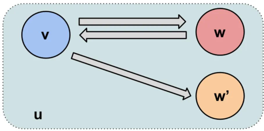
(22) 1.2. PHOTONIC DELAY SYSTEMS. 3. 1.2. Photonic delay systems Despite the ubiquity of delay systems, a large contribution to the study of delay dynamics have been made through semiconductor laser systems. The versatility, compactness and robustness of their performance made semiconductor lasers ideal test-beds for the study of nonlinear dynamics, and in particular, good representatives for the study of delay systems. Since the invention of semiconductor lasers in 1962 [8, 9, 10], their use has been expanding to endless applications and technological advances, making the research in the field of photonics a continuing emerging area with a substantial economic impact. Semiconductor lasers are characterized by a strong sensitivity to delayed feedback or delayed coupling, meaning that, even when a tiny fraction of light reenters into the cavity of the laser, the emission properties are significantly perturbed [11, 12, 13, 14]. The feedback induced instabilities result in the emergence of complex dynamical scenarios, far from the stable steady emission expected from a laser. Such complex dynamics have been investigated extensively [15, 16, 17, 18]. Nevertheless, the original motivation for its study was to get rid of most of the delay-induced dynamics, since their presence implies the degradation of the performance in real-world applications like the CD/DVD players or in telecom modules. It was in the early 1990s that their advantageous attributes started to be recognized, mainly in the field of chaos applications [17, 19]. With the fast time scales of the chaotic oscillations over frequencies of gigahertz, the instabilities in semiconductor lasers turned out to be an important attribute for modern chaos communications [20] or chaos encryption [21, 22], but also as low-coherence sources for rainbow refractometry [23], remote position sensors, lidars [24], random bit generators [25] or information processing [26], among many others. It is worth mentioning that complex dynamics is here understood as all nonlinear dynamical phenomena emerging from the delayed feedback [27, 28, 29, 30, 31]. Periodic oscillations [32, 33] and period-doubling [34, 35], quasi-periodicity [36], deterministic chaos [37, 38, 39, 40, 41, 42, 43, 44, 45, 46], multistability [38], bifurcation cascades [47, 48, 49], intermittency [50], and chaos synchronization [51, 52, 53] are some of the nonlinear behaviors observed in photonic delay systems.. 1.2.1 Photonic delay systems in the drive-response scheme Semiconductor lasers are not only sensitive to their own delayed feedback but the addition of an external driving signal to the laser also perturbs the emission properties. Photonic delay systems represent a good platform for the investigation of drive-response schemes. In such schemes, the drive system generates an output signal that is sent to the response system, which in this case is a system with delay (see Fig. 1.1 (a)). Then, the reactions of the response system to the drive are analyzed. The drive is usually a direct parametric modulation of the laser pump current, but more elaborated drives can be utilized. A delay system can also act as a drive when its output is injected into a response system (which can be a delay system or not), as illustrated in Fig. 1.1 (b). One could even think of a single laser with delay feedback.

(23) 4. CHAPTER 1. INTRODUCTION. as self response system, where the output signal x(t) is the response to the drive x(t-τ ) like in Fig. 1.1 (c). In a more elaborated setup, a single delay system with multiple feedback loops could serve as a drive and response system at the same time (see Fig. 1.1 (d))). While the use of an external driving signal restricts the origin of the drive to electrical scalar recorded waveforms, the possibility to use photonic delay systems also as drives (Fig. 1.1 (b), Fig. 1.1(c) and 1.1(d)) permits the utilization of complex continuous vector-state optical drives. Along this Thesis, different schemes of drive-response systems are used. The drive-response configuration represents a prominent base for the investigation of a crucial property of nonlinear systems: consistency.. Figure 1.1: Illustration of four possible schemes employed for the investigation of driveresponse systems. The delay system is used as response system. (a) Any arbitrary signal can be used as a drive. (b) The output of a delay system serves as the drive of a response system, which can be a delay system or not. (c) A single laser as self response system. (d) A delay system with two feedback loops.. 1.3. About Consistency In real life applications, it is an obvious requirement to have a reliable operation of a given system. This means assuring the same (or very similar) performance of the system when tested repeatedly. In nonlinear dynamical systems, we call this property consistency. Consistency is defined as the ability of a nonlinear system to respond in a similar manner to similar inputs [19]. This definition can be easily interpreted in terms of drive-response schemes, so that similar drives lead to similar responses, without imposing any restriction on the types of drive signals used. The nature of the drive signals can be optical or electrical, and their.

(24) 5. 1.3. ABOUT CONSISTENCY. origin can come from real recorded time traces of the system, from noise, from artificially generated waveforms with an Arbitrary Waveform Generator, or any other source. Consistency is, therefore, a non-trivial property of the response system that depends on the drive. For a certain input, a system might provide a consistent response, whereas the same system can exhibit inconsistent behavior for another drive. This is illustrated in Figure 1.2.. Drive. Response Consistent. Inconsistent. Figure 1.2: Illustration of the concept of consistency. The same system can exhibit consistent or inconsistent responses depending on the drive. When repetitions of the same drive lead to a similar response, there is a consistent behavior of the system. But if repetitions of a drive signal lead to significantly different responses, the system is inconsistent. The boundaries between consistent and inconsistent behavior are not well defined, and the responses of a dynamical system can be classified into a certain degree of consistency. Responses that are structurally similar but not identical can still be considered consistent. But in a more restrictive scenario, we can distinguish complete consistency as the case in which the same input leads to the exact same output of the system. Consistency has also been referred to as reliability and often investigated under the terms of generalized synchronization or noise synchronization [54]. In Chapter 2, the concept of consistency with the notion of generalized synchronization is discussed.. 1.3.1 Applications of consistency There is a clear connection between consistency and the analysis of brain dynamics. The brain, although a complex system, exhibits various degrees of consistency in the neuronal functionality in response to repetitions of input signals and stimuli [55]. This phenomenon has commonly been referred under the term reliability. Consistency also partakes in the formation of spatio-temporal patterns in motor learning [56]. The investigation of the fun-.

(25) 6. CHAPTER 1. INTRODUCTION. damental mechanisms behind the achievement of consistency can be useful to understand brain dynamics and the process of learning in the brain. Neuronal systems and photonic delay systems share some common phenomena that make the latter good candidates for such investigations. Both systems can exhibit zero-lag synchronization despite their delays in propagation, and the topology of the configuration is also crucial in both systems for the achievement of synchronization dynamics. The many similarities between the dynamical properties of neuronal networks and photonic delay systems have also led to the development of a bio-inspired information processing concept, the so called Reservoir Computing, whose performance strongly depends on the consistency properties.” In Reservoir Computing, a nonlinear delay system has been proposed and demonstrated successful for the performance of complex tasks such as speech recognition [26, 57]. The method uses the scheme of drive-response system, and a consistent (or reliable) response output with respect to a drive signal is required for the successful implementation of this machine-learning tasks. However, the uses of consistency surpass the processing of information. Consistency is a concept that shows up in many other fields where the scheme driveresponse is present. The success of many practical applications relies on the reproducibility of the dynamical behavior to guarantee the robustness of the system. In biology, the response of biomolecules to external inputs can be tested and used to identify severe changes in the system. In engineering, a consistent behavior is a basic requirement for the development of new materials when assessing their mechanical properties. It is also essential in cryptography for the generation of secure tokens, where the drive-response relation must be complex and at, the same time, reproducible [19]. So far, we have introduced the property of consistency in nonlinear systems. A semiconductor laser system with delay can display a complex yet reproducible behavior and, thus, predictable. Interestingly, and as explained in the next section, the same system can also act as a source of unpredictable dynamics, broadening the uses of photonic delay systems.. 1.4. About Unpredictability Among the different dynamics generated by photonic delay systems, deterministic chaos is one of the most prominent and investigated behaviors. Chaos is a phenomenon characterized by irregular oscillations in a nonlinear system with a strong dependence on initial conditions [58]. This means that any two trajectories that start close to each other will separate exponentially with time, Figure 1.3. Nevertheless, chaos is deterministic which means that, if the initial conditions are known with infinite precision, the irregular behavior can be reproduced. Knowing the initial conditions without error is an inherently unrealistic abstraction in continuous dynamical systems but, still, chaos should not be taken as a synonym for randomness or stochasticity..

(26) 1.4. ABOUT UNPREDICTABILITY. 7. Figure 1.3: Sensitivity to initial conditions: two trajectories that begin close to each other separate exponentially with time. In practice, the distinction between a random and a chaotic process from experimental data can be a hard task to achieve. Often, the methods rely on tracking the evolution of two nearby trajectories but the identification of close states in high dimensional systems demands big amounts of data and computations. In photonic systems, semiconductor lasers with time delayed feedback produce fast dynamical instabilities that can lead to deterministic chaos. Semiconductor lasers with delayed feedback, as real chaotic systems, also exhibit a stochastic contribution in their dynamics. Noise additions from the spontaneous noise emission of the laser, and also from the experimental devices that form the setup, are unavoidable. The noise is amplified due to the inherent nonlinearity of the system giving rise to random-like dynamics. Therefore, it is the actual interplay of chaos and noise that makes these systems an outstanding implement for unpredictable behavior.. 1.4.1 Applications of unpredictable dynamics In a world in which digital technologies are established in our everyday lifes, the demands for security in network communications and data transmission have led to the development of new encryption protocols. The use of the chaotic dynamics of semiconductor lasers represents a good approach, given the possibility to operate at high speeds and their easy implementation in current optical communication channels. One current application that benefits from the combination of chaotic dynamics with inherent noise is random bit generation [25]. The chaotic output of a semiconductor laser is sampled with a fast oscilloscope, converted into a stream of binary numbers and postprocessed, resulting in random bits that can pass sophisticated tests of randomness. We elaborate on this application in Chapter 6, in which a practical implementation of a fast random bit generator based on a laser with polarization rotated feedback is demonstrated. Another important application is chaotic secure communications based on chaos synchronization between two nonlinear systems [22, 59, 60]. Two independent chaotic laser systems.

(27) 8. CHAPTER 1. INTRODUCTION. exhibit different autonomous dynamics due to the uncertainty in their initial conditions. However, the two systems can synchronize when coupled, that is, when a small portion of the chaotic output from one system is injected in to the other. This principle serves as the key for chaotic encryption and decryption of messages and secure exchange of a private key through a public channel [61, 62]. Other uses of chaotic lasers in optical sensing include the correlation or chaotic radar (CRADAR) based on chaotic pulse trains with high pulse repetition frequencies that allow for high precision range measurements [63, 64]. In the field of computing, optical logic gates have been implemented via the synchronization properties of two chaotic lasers [65]. These applications are only a few examples of the possibilities of chaotic photonic systems. New exciting developments of chaotic dynamics in semiconductor lasers are yet to come. 1.5. Overview of this Thesis The work in this Thesis is devoted to the study of photonic delay systems as a source of a great variety of complex dynamics that can ensure reliable behavior as well as unpredictability. The property of consistency is investigated from a fundamental point of view with the characterization of the responses from different laser systems and driving sources. The unpredictability property is exploited in the cryptographic application of random bit generation. • In Chapter 2, we present the methods and tools used to quantify consistency and unpredictability, and discuss the relation between consistency and generalized synchronization. • In Chapter 3, we investigate the consistency properties of a semiconductor laser system to its own time-delayed signal. A scheme with two different feedback loops is utilized to store a copy of the dynamical features with high precision and inject it at a later time. The consistency is quantified in terms of correlations and, for the first time in experiments, with a measure proportional to the sub-Lyapunov exponent, the σ value. • In Chapter 4, a laser with delayed feedback, operating in the regime of Low Frequency Fluctuations, is employed for the characterization of consistency to an external drive in the form of short pulses. The feasibility of induced intensity dropouts in the dynamics is analyzed with different pulse distributions. The inter- and intra-correlations are calculated to demonstrate the role of the drive pattern. • Chapter 5 covers the use of an opto-electronic intensity oscillator to explore its consistent behavior when different external drives are applied. As a scalar system with multistability, new dynamical features emerge under the influence of a drive. Harmonic signals, pseudo-random pulses and time-traces originating from the system are used as modulation. The correlations indicate a significant level of consistency even in a global chaos regime..

(28) 1.5. OVERVIEW OF THIS THESIS. 9. • Chapter 6 focuses on the exploration of unpredictable dynamics from a laser system to the application of random bit generation. Optimum operating conditions are identified, and guidelines on the interplay between dynamics, acquisition process and postprocessing procedures are discussed to guarantee the randomness of the bits. • The last Chapter of this Thesis includes a summary of the achievements, and an outlook and perspectives for future work..

(29) 10. CHAPTER 1. INTRODUCTION.

(30) CHAPTER. 2. Concepts and tools It is a recurring experience of scientific progress that what was yesterday an object of study, of interest in its own right, becomes today something to be taken for granted, something understood and reliable, something known and familiar − a tool for further research and discovery. J. Robert Oppenheimer, Physicist. This Chapter covers the mathematical tools employed to quantify consistency and unpredictability throughout the Thesis. Regarding the concepts, a discussion on the equivalence between consistency and generalized synchronization, two closely related terms, is also included. To measure consistency, we introduce the sub-Lyapunov exponent, used in Chapter 3, and the inter- and intra-correlations, employed in Chapters 4 and 5. These two quantities provide different and valuable information about the responses of a driven system. In the last section, we review the well-established tools available to quantify unpredictability, like entropy or autocorrelation function, and we discuss other indicators of the randomness of a time series. 2.1. Consistency and Generalized Synchronization Consistency is often put in context with generalized synchronization [66, 67, 68]. It should be noted that differences between the interpretations of consistency and generalized synchronization need to be taken into account, and the two terms cannot be utilized synonymously. Generalized synchronization in driven systems is understood as the existence of a functional relationship between the state of the driven system y with another dynamical system x that 11.

(31) 12. CHAPTER 2. CONCEPTS AND TOOLS. acts as the arbitrary drive (Fig. 2.1 (a)).. x (a). y. x (b). y y’. Figure 2.1: (a) Drive-response scheme for generalized synchronization. (b) Scheme for the extended generalized synchronization with a replica system y ′ . Consistency and generalized synchronization already present a major dissimilarity in the point of view: generalized synchronization describes a property of the relationship between coupled systems while consistency is a property of the response system. The fact that the definition of consistency is based on the ”similarity” of the responses makes it a difficult concept to be described and quantified mathematically. Whereas consistency implies a broad set of possible outcomes, ranging from inconsistent to complete consistent responses, generalized synchronization only contemplates a subset of consistency: complete consistency. In the drive-response scheme like the one depicted in 2.1 (a), complete consistency and generalized synchronization are indeed equivalent. If the drive and response systems are in a state of generalized synchronization, in which stability is implied, the responses to the drive will have complete consistency and viceversa. Nevertheless, if the responses are not completely consistent, but have a high degree of consistency, the system will not exhibit generalized synchronization. This could be the case, for instance, when the responses are not identical but are still narrowly bounded. If we extend the concept of generalized synchronization, as in the Abarbanel test [67], we can denote as extended generalized synchronization the situation in which a copy of the system y ′ subject to an arbitrary drive x receives the same input and, thus, exhibits complete synchronization with the original y, as depicted in Fig. 2.1 (b). With this scheme, the replica system y ′ serves to test the repetition of the input x. Again, the three properties (generalized synchronization between x and y, complete synchronization between y and y ′ , and complete consistency of y) would be equivalent. However, as soon as we leave the unidirectional scheme x ⇒ y to other arbitrary schemes, the equivalence between properties becomes non-trivial. For example, a mutually coupled scheme x ⇔ y can already alter the possible outcomes. The functional relationship between the states of drive and response may be undefined, but x and y may still be consistent when the replicas are attached, and viceversa. To summarize, the extended generalized synchronization is equivalent to complete consistency as a local property of a driven system, no matter the origin of the drive. When the scheme is not a unidirectional drive-response setup, the equivalence between the two concepts.

(32) 13. 2.2. TOOLS TO MEASURE CONSISTENCY. does not apply anymore, and the presence of a generalized synchronization manifold does not imply consistency. 2.2. Tools to measure consistency There are different ways to measure consistency that take into account the type of drive. Here, we introduce two different tools to quantify the degree of consistency. One is based on the calculation of the sub-Lyapunov exponent, and the other is based on the calculation of correlations. The sub-Lyapunov exponent characterizes the response of a driven system in terms of stability and requires the access to the error between the two response signals. The sensitiveness to mismatches between the two responses makes this method more oriented to non-scalar high optical bandwidth drives that can be repeated with high accuracy. The calculation of the correlation coefficient between responses is a practical method that can directly quantify the level of consistency. Their fast computation times and the possibility to use them to identify patterns in the responses makes it more suited for external scalar drive signals that are reinjected multiple times.. 2.2.1 The sub-Lyapunov exponent In dynamical systems, and particularly in chaotic systems, the sensitivity to the initial conditions is often described by the Lyapunov exponent λ, which measures the mean rate of the separation between two nearby trajectories. For a given dynamical system with a state vector x(t) evolving like in Eq. 2.1:. ẋ(t) = f (x(t)). x(t) ∈ ℜd. (2.1). we can linearize the temporal evolution of a small separation (or perturbation) δx(t): ˙ δx(t) = Df (x(t)) · δx(t). (2.2). so that for a given trajectory x(t), the maximal Lyapunov exponent is defined by:. λ = lim. t→∞. ||δx(t)|| 1 ln{ }. t ||δx(t0 )||. (2.3). There is a whole spectrum of Lyapunov exponents, which in the case of an autonomous system, equals the dimensionality of the phase space (or in other words, same number of Lyapunov exponents as system variables). In delay systems though, the spectrum of Lyapunov exponents is formally infinite. However, we focus on the maximum Lyapunov exponent,.

(33) 14. CHAPTER 2. CONCEPTS AND TOOLS. which gives a notion of the predictability of the system and connects the local stability with the global dynamics. A positive maximal Lyapunov exponent indicates chaotic dynamics. A negative maximal Lyapunov exponent is associated with a steady state dynamics, and a λ=0 could indicate a periodic or quasi periodic orbit in phase space. The Lyapunov exponents are a property of the system, which allow for other derived measures like the Kolmogorov-Sinai entropy or the Kaplan-Yorke dimension, related to the complexity and dimensionality of the system. Pecora and Carroll [51] introduced the concept of the sub-Lyapunov exponent as a property of a subsystem belonging to a chaotic system. To investigate the synchronization properties of chaotic coupled systems, they considered an autonomous system with phase space vector u and divided it into two subsystems v, w. The subsystems obey the equations of motion: v̇(t) = g(v(t), w(t)) ẇ(t) = h(v(t), w(t)). (2.4). They observed that, under certain conditions, a copy of w, w′ , can be made to synchronize with the original w if both receive the same signal. To prove it, they followed a similar approach, linearizing with respect to w and writing the equations for a small perturbation of the synchronized state ξ(t):. Figure 2.2: An autonomous system u is divided into two subsystems u = u, w and a copy w′ is created to test the synchronization properties.. ˙ = Dw h(v(t), w(t)) · ξ(t). ξ(t). (2.5). From this equation, the maximal Lyapunov exponent of the subsystem can be obtained, also known as sub-Lyapunov exponent λ0 :.

(34) 2.2. TOOLS TO MEASURE CONSISTENCY. 1 ||ξ(t)|| ln{ }. t→∞ t ||ξ(t0 )||. λ0 = lim. 15. (2.6). When λ0 is negative, there is complete synchronization between w and w′ . There are as many sub-Lyapunov exponents as dimensions of the subsystem w. One can identify this system as a drive-response scheme, in which an autonomous subsystem acts as the drive of another subsystem, the driven system. For the latter, the maximal sub-Lyapunov exponent can be defined, and measures the convergence of the response states to a function of the drive. In this Thesis, all the schemes investigated are delay systems, with a temporal evolution given by Equation 1.1. The sub-Lyapunov exponent of delay laser systems quantifies the consistency with respect to small perturbations in the response of a semiconductor laser subject to its own time delayed feedback. The sign of the sub-Lyapunov exponent determines whether the laser behaves in the same way when the external input is repeatedly applied, so that a negative λ0 would indicate an exponential decay rate of the small perturbation to the consistent state. The sub-Lyapunov exponent has been linked to the concept of strong and weak chaos. These two terms refer to two different types of chaos identified in networks of time-continuous systems with time-delayed couplings. Thus, delay instabilities can be categorized depending on the scaling properties of the maximal Lyapunov exponent [69, 70]. In the large delay times, the maximal Lyapunov exponent converges to a nonzero value in the presence of strong chaos but, in the case of weak chaos, the maximal Lyapunov exponent scales with the inverse delay time. From the point of view of delay systems in the drive-response scheme, the sub-Lyapunov exponent represents a direct measurement of the type of chaos. A positive syb-Lyapunov exponent indicates strong chaos dynamics, while a negative sub-Lyapunov exponent implies weak chaos. For synchronization purposes, it has been shown that only networks with weak chaos can synchronize to a chaotic signal. The sub-Lyapunov exponent is also defined outside delay coupled networks, which then emerge as a special case of driveresponse systems if the delay couplings are considered as drives for the individual nodes. Using the extended notion of the sub-Lyapunov exponent, an analogue to weak chaos can be identified with the complete consistent response, and strong chaos with a non-completely consistent response. Jüngling [71] developed an algorithm to extract the value of the subLyapunov exponent from stationary chaotic time series of a delay system. In Chapter 3, a method to measure a quantity proportional to the sub-Lyapunov exponent, σ, is explained in detail.. 2.2.2 Inter- and intra-correlations Complementary to the widely used correlation coefficients, in the cases where an external modulation is repeatedly injected to the system, we use the so-called inter-correlation and.

(35) 16. CHAPTER 2. CONCEPTS AND TOOLS. Figure 2.3: Illustration of the concepts of inter- and intra-correlations. Two trajectories are depicted in response to a pulsed drive. 4 responses uji (t) of duration T are compared within the same time trace (intra-correlation) and among the two repetitions (inter-correlation). intra-correlation measures. The input drive can be an harmonic function, a random distribution of pulses or even a noisy signal, with or without periodicity. The intra-correlation compares the response trajectories of the system along the same input drive, whereas the inter-correlation compares the responses across multiple repetitions of the same input drive. These two types of correlations, developed by Jordi Garcı́a-Ojalvo and Javier Buldú, are illustrated in Figure 2.3. Let the drive be a sequence of N pulses or an harmonic function of N periods, and M the number of time traces corresponding to the repetitions of the modulation sequence. We denote the response of the system to a given pulse or period as uji (t) with t ∈ [0, T ]. Here, i indicates the repetition of the sequence, so that i ∈ [1, M ], and j ∈ [1, N ] defines the index of the pulse or period along the sequence, so that N T is equivalent to the total duration of the sequence. The duration of the responses T coincides with the period of the modulation or the minimum spacing between pulses. To compute the correlations, we altered the original expression of the pairwise-based Pearson coefficient. For two given responses, uji and ulk , the Pearson coefficient would be.

(36) 17. 2.2. TOOLS TO MEASURE CONSISTENCY calculated as: Cuj ,ul = i. h(uji − µuj )(ulk − µul )i k. i. σu j σu l. k. i. (2.7). k. 2 The new expression uses a global mean µglobal and variance σglobal instead of product of individual standard deviations:. Cuj ,ul i. k. h(uji − µglobal )(ulk − µglobal )i , = 2 σglobal. (2.8). where µglobal is the mean of the ensemble of all the responses. In this global normalization, all the responses are concatenated into a time series, and then normalized as a whole. In the case of a pulsed drive, it excludes the pulses. This causes a centering around zero that highlights the small differences in the amplitudes of the responses. This new method to compute correlations is capable to highlight subtle changes between responses that, with the locally normalized coefficient, would have remained hidden. An example of this could be two responses characterized by a positive growth of the power intensity but with different slopes. The new global centering would distinguish the two types of responses with a lower correlation 2 one uses value than the Pearson coefficient. Whether for the calculation of µglobal and σglobal the time traces excluding the pulses, or just the portions of time traces corresponding to the windows used for the correlation, is a free choice. In the following, the results shown correspond to the second case. The final correlation would then be given by the average of all the pairwise calculated values. We can now define the intra-correlation as the correlation for responses along the same sequence: M. Cintra =. M. N. N. X X X X h(uj − µglobal )(ul − µglobal )i 1 i k 2 M N (N − 1) σglobal. (2.9). k=1 i=k l=1 j=1 j6=l. This formula calculates, for every repetition i of the drive, the correlation of each response window with the rest of the responses, excluding the self ones. The inter-correlation is defined as the correlation for the same response window across different repetitions of the drive: M. Cinter =. M. N. N. X X X X h(uj − µglobal )(ul − µglobal )i 1 i k . 2 M N (M − 1) σglobal. (2.10). k=1 i=1 l=1 j=l i6=k. Equation 2.10 calculates the correlation of the same response window l across the multiple repetitions k of the drive, excluding the self ones. There is another way to compute these correlations with less computational demand based on an ensemble of responses, where the term ensemble refers to the set of all responses. For.

(37) 18. CHAPTER 2. CONCEPTS AND TOOLS. that, the ensemble needs to be centered and globally normalized. The normalization should be performed again as if all the responses were concatenated to a new time series. The criteria can be expressed as: ZT 1 X1 dt uji (t) = 0 MN T. (2.11). ZT 1 X1 dt(uji (t))2 = 1. MN T. (2.12). i,j. i,j. 0. 0. A well-behaved intra-correlation based on the globally normalized ensemble compares all the individual responses, similar to the pairwise correlation coefficient, and averages over the repetitions. T. Cintra. XXZ 1 = dtuji (t)ulk (t) (N 2 − N )M 2 T. (2.13). j6=l i,k 0. This formula correlates all the individual responses without excluding any particular combination except the self one. Limiting the intra-correlation to calculations within the same sequence would only affect the normalization factor. Analogously to the intra correlation, the globally normalized inter-correlation can be written as: T. Cinter. XXZ 1 dtuji (t)ulk (t). = (M 2 − M )N T. (2.14). j6=l i,k 0. However, another helpful expression can be derived for the calculation of the intercorrelation through the distance of the individual responses to their mean, which gives an idea of the ensemble spread. We can write the ensemble mean ũj that depends on the event j: ũj =. 1 X j ui (t). M. (2.15). i. And we can calculate the distance of the individual responses to their ensemble mean as: Dj2 (t) =. 1 X j (ui (t) − ũj (t))2 . M. (2.16). i. It can be shown that the distance of a response to the ensemble mean is connected to the inter-correlation like:.

(38) 19. 2.2. TOOLS TO MEASURE CONSISTENCY. T. Cinter. Z 1 1 X =1− dtDj2 (t). 1 − 1/M N T j. (2.17). 0. where the normalization factors contemplate the projection of all the responses to a certain event onto each other excluding the self-projection. This is a useful expression that permits to split the correlation into meaningful contributions and distinguish for an event-dependent correlation. The inter- and intra-correlations are very intuitive measures for consistency. A high correlation value would indicate a consistent response of the system, whereas a low correlation value would suggest an inconsistent response. The inter-correlation is an indicator of the reproducibility of the amplitude pattern for a given response. A correlation of 1 would correspond to a complete consistent response, meaning that the responses would overlap into a narrow line. With a correlation of 0, the ensemble of responses would display an unstructured distribution. The intra-correlation compares responses to different events. This might be of interest to identify whether consistency depends on the occurrence of a certain event or, on the contrary, the system responds consistently to any sort of perturbation. The first case should translate into a high inter-correlation and lower intra-correlation, while the latter should display similar inter- and intra-correlations. This method also allows for a whole gradient of consistency, and can provide insights into the memory capabilities of the system when the repetitions are compared. Inter- and intra-correlations also unveil important information on the statistical properties of the nonlinear system. Using a pseudorandom pulsed sequence as example of modulation, every occurrence of a pulse is acting as a trigger for the evaluation of the responses. If one interprets the inter-correlations as an ensemble average of the responses, provided that it uses repetitions from the same trigger, and the intra-correlations are considered a time average between different responses from different trigger points, the inequality between the two quantities would reveal that the system is not ergodic in this sense [72]. Focusing on the intra-responses, their dissimilarity can illustrate the time scales at which the memory effects remain. If the separation between the pulses were long enough, the trajectories would have enough time to reach the attractor after the perturbations, and therefore, we would not expect much difference between the inter- and intra-correlations. But in cases in which the influence of the previous pulses is visible, the time scale of the memory is larger than the intervals between the perturbations, preventing the trajectories to reach the stable attractor. Hence, under such circumstances, the inter-correlation values are higher than the intra-correlations.. 2.2.3 Review of the consistency measures Consistency is a property that lacks a rigorous definition so far and, consequently, of a mathematical framework with clear tools to quantify it. All the measured quantities rely on the.

(39) 20. CHAPTER 2. CONCEPTS AND TOOLS. definition of consistency based on the similarity between responses, but no clear boundaries between inconsistent, consistent and complete consistent response have been determined. Depending on the drive-response system, different measures are suited to estimate the degree of consistency. Calculation of correlations in their different forms (Pearson coefficient, distance to a response, autocorrelations or distinguishing inter- and intra-correlations), have been employed to indicate the similarity of the responses. Their use is motivated by the ability to extract these quantities from experimental recorded data, specifically, from time traces of the dynamics. Their interpretation is also very straightforward. The consistency correlation, understood as the correlation between responses (either inter or intra) to a repeated drive, is a meaningful measure that allows for a whole range of consistency, scaled from zero to one. A Pearson coefficient close to one also indicates that two responses are almost identical, but does not take into account differences in the offset of the responses. In a single system with delayed feedback, in which the delayed signal acts as an external drive, the autocorrelation function can be interpreted as a consistency measure too. The height of the delay echoes imply a high similarity in the trajectories, and thus, a consistent response to the self-delayed input. All these measures can be good indicators of the consistency properties, although there are situations in which they might fail. For instance, experimental issues, like a poor signalto-noise ratio, can easily induce inaccurate correlation values. In the case of a behavior, which in an ideal system would be completely consistent, the presence of mechanisms that could temporally alter the synchronization of the responses, such as bubbling, could lead to low correlation values, which would then be interpreted as not complete consistency or even inconsistency. The sub-Lyapunov exponent is the quantity at the core of complete consistency, characteristic for the drive-response schemes. It affects the consistency properties of the response system and, in the case of delayed feedback systems, connects them directly with strong and weak chaos. In other words, the sub-Lyapunov exponent describes the conditional stability of the response of a dynamical system with respect to a certain drive. When the drive is a delayed feedback signal, a negative λ0 indicates the presence of weak chaos. Under such circumstances, the response of the driven system is stable and can be consistent. With a positive λ0 , we operate in a regime of strong chaos and the response of the unit is not completely consistent. Yet it is difficult to extract the sub-Lyapunov exponent from experimental time traces. Testing the consistency properties out of the complete consistency case becomes more intricate. The distinction between a high degree of consistency and inconsistency is not possible from the sub-Lyapunov exponent. Consequently, we recommend, when possible, a combination of both methods to characterize the consistency properties of the laser system. With the extraction of the sub-Lyapunov exponent and the correlation measures a good description of the consistency in a dynamical system can be achieved. Future methods to extract the sub-Lyapunov exponent, as well as the development of new tools to quantify consistency, will improve significantly the characterization of nonlinear systems..

(40) 2.3. TOOLS TO MEASURE UNPREDICTABILITY. 21. 2.3. Tools to measure unpredictability Unpredictability is commonly measured by entropy rate [73]. In chaotic systems, unpredictability arises from the strong dependence on the initial conditions, so that small perturbations grow exponentially with time, limiting the abitility to predict future states. This sensitivity of the system to initial conditions can be quantified by the Kolmogorov-Sinai entropy, which is bounded by the sum of all positive Lyapunov exponents. hKS ≤. X. λi. (2.18). λi >0. Given that any microscopic noise in the chaotic system amplifies the divergence of two nearby trajectories in phase space, chaotic systems can generate random information [74, 75]. In the context of information theory, Shannon’s formula for the entropy rate characterizes how quickly the system generates unpredictable information [76]: H(t) = −. 1 X. Pi (t) log2 Pi (t). (2.19). i=0. where Pi (t) is the probability of occurrence of bit i (0,1) at the time t. As time evolves, the Shannon entropy increases, indicating a growth of uncertainty due to the spread of trajectories, and relates to the Kolmogorov-Sinai entropy. From experimental data, one can digitize the signal on one bit, so the chaotic dynamics can ideally generate up to one bit of entropy at a rate determined by the Lyapunov exponent. The time required for the system to reach an entropy value equal (or very close) to 1 is known as the memory time of the system. By computing these quantities, one can estimate the rate at which random bits can be generated. Entropy calculations have also been used to explore the deterministic and stochastic aspects of a laser system used for random bit generation [74, 75]. Nevertheless, there are other measures that give an account of the unpredictability in the dynamics. The autocorrelation function has been used to estimate the predictability: if future values of a time series depend on current and past values, the time series is predictable, and the dependence will show up in the autocorrelation function. The autocorrelation between times t and s for a process x is defined as:. AC(s) =. < [x(t)− < x(t) >][x(t − s)− < x(t) >] > < [x(t)− < x(t) >]2 >. (2.20). The autocorrelation function of the output of a semiconductor laser subject to delay feedback will present delay signatures at lags of the delay time τ . The height of the delay echoes serves as an indicator of the existence of repeating patterns in the dynamics, so a complete suppression of the correlation peak is desirable. This property can also be formulated as the.

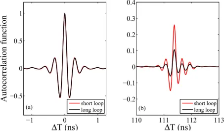
(41) 22. CHAPTER 2. CONCEPTS AND TOOLS. preference to operate in strong chaos conditions. The memory time effects of the system are also contained in the decay of the zeroth autocorrelation peak, providing insights into the independence of successive data points [77]. In addition to the autocorrelation function, the mutual information can be used to measure the uncertainty in the dynamics. The unpredictability property of chaotic laser systems is mostly used in cryptographic applications, where the output of the laser needs to be chaotic, and to satisfy some noise-like features. The observation of some properties, although it cannot quantify the unpredictability, is key to guarantee a random behavior. The probability distribution functions of time series provide information about the appropriateness of the dynamics for unpredictability. Symmetrical distributions that resemble a Gaussian distribution are more favorable, and considered a good starting point for most chaotic applications. In terms of frequency components, the spectrum of an unpredictable time series should be broad, and have a flat power spectral density, similar to the white noise spectrum [77]. Other methods to estimate the unpredictability include the already mentioned calculation of the maximal Lyapunov exponent, the Kaplan-Yorke dimension or the phase space reconstruction of an attractor using data [19, 74, 75, 78]..

(42) CHAPTER. 3. Consistency of a semiconductor laser to its own time delayed feedback “The range of nonlinear dynamics is often largely underestimated.” Thomas Jüngling, Physicist.. 3.1. Introduction Consistency in dynamical systems has proven to be a powerful concept due to the ubiquity of drive-response schemes in nature and technology. The ability to respond in a similar way to similar inputs, starting each time from different initial conditions, is a necessary condition for the reliable operation of the systems. Cognitive tasks in neuron dynamics [79] or bioinspired information processing [26, 57, 80, 81, 82] strongly depend on a consistent behavior. The first experimental work on consistency was introduced in 2004 by Uchida et al.[83]. In their experiment, a laser system is driven repeatedly by the same drive signal in order to describe the reproducibility of the responses. Recent numerical and experimental advances on consistency [84, 85, 86] also comprise the characterization of generalized synchronization properties of laser systems (see Chapter 1) driven by common light sources with fluctuating phase and or amplitude [87, 88, 89, 90, 91]. In this Chapter, we focus on two aspects of consistency that are critical for a controllable application. The first is the development of an experimental scheme providing a high quality repeated drive for fast experimental systems. To extend the investigations on consistency beyond the use of electrical drives, we need to design an experiment that allows to store non-scalar drives, such as optical signals, and inject them again while preserving the high optical and dynamical bandwidths. To achieve this, we employ a configuration of a photonic delay system with multiple feedback loops. 23.