TWO-DIMENSIONAL MESH OPTIMIZATION IN
THE FINITE ELEMENT METHOD
R. MARTINEZ and A. SAMARTIN
Abstract-The solution to the problem of finding the optimum mesh design in the finite element method with the restriction of a given number of degrees of freedom, is an interesting problem, particularly in the applications method. At present, the usual procedures introduce new degrees of freedom (remeshing) in a given mesh in order to obtain a more adequate one, from the point" of view of the calculation results (errors uniformity). However, from the solution of the optimum mesh problem with a specific number of degrees of freedom some useful recommendations and criteria for the mesh construction may be drawn. For 1-D problems, namely for the simple truss and beam elements, analytical solutions have been found and they are given in this paper. For the more complex 2-D problems (plane stress and plane strain) numerical methods to obtain the optimum mesh, based on optimization procedures have to be used. The objective function, used in the minimization process, has been the total potential energy. Some examples are presented. Finally some conclusions and hints about the possible new developments of these techniques are also given.
INTRODUCTION
The finite element method (FEM) represents a well-known procedure for efficiently solving field prob-lems. Many computer programs based on this method are available for solving very general prob-lems. In spite of this extraordinary development, some important problems of this method demanding further study still remain. In general, these problems are related to the quality level of the FEM results. In fact, during the past decade considerable research effort has been devoted in order to obtain some practical estimations of the error produced in FE results [1-3]. An important user's decision in relation with this error lies on the choice of the node locations in a FE mesh.
Current research is attempting to find automatic techniques to improve, in some sense, an already existing mesh by adding new degrees of freedom (new nodes or increasing the order of the polynomial in some elements). Thus a better mesh than the original is reached, because error can be nearly constant over the whole domain of the FE analysis.
In this paper, the problem of finding an optimal mesh will be considered, i.e. to find the node locations of a given topological FE mesh with a fixed number of degrees of freedom. The solution of this problem can be used to give some recommendations and guidelines for designing FE meshes.
This problem has been treated in the first FE error analysis. In this respect ref. [4] can be considered as a pioneer. Some results of this first research period suggest some relation between the node positions in the optimal mesh and the density of the strain energy at the node (6, 7]. In this paper some of these con-clusions are presented and other alternative tech-niques are hinted upon. From the results obtained
recommendations for the design of the optimal mesh are also provided.
1-D PROBLEMS: CLOSED-FORM SOLUTIONS
The first group of problems that can be solved by analytical means corresponds to the mono-dimen-sional field problems of class C0
• The rod under axial force is a well-known example of this type of prob-lem. In the case of a rod with constant cross-sectional properties, the optimal FE mesh obviously corre-sponds to the equal distance between two consecutive nodes. For this reason the next more complicated case is envisaged, namely, the rod with variable cross-sectional properties for which the optimal mesh is not known beforehand.
The most simple longitudinal variation of the cross-section corresponds to the linear one. This example will be treated below. The problem, rep-resented in Fig. I, to be solved is mathematically described as follows: the equation in the domain is
:x(EA~:)=p(x),
atxE(O,L) (1].The essential boundary conditions are u =u1, atx =0
U=U
2 ,atx=L.
The natural boundary conditions are du
EA-
= - p1 , atx
= 0 dxdu
y
:
I I I I
I A2
I X
~---~---~-~--->~
CD
I
®
~Ul
I I I I
~---~---~
i A1
A2 ... ... ... ... ....
..
....
...
Cif
"'
.,.
.,.
.,.
/'@
~
Fig. I. One-dimensional problem.
In this particular case the linear cross-sectional
vari-ation is given by the equation
The main results of this problem are summarized as follows: stiffness matrix
(I)
The initial solution corresponding to the ·constant
distributed load p(x)
=
q (constant) along (0, L) andto null displacements at the boundaries (u1
=
0, u2 =0)where the constants h and p are defined for the expressions
7i
= 2J,lln((l
+
Jl)/(1 - Jl)] - Jl+
Ip =
-2J,l ln((l
+
p.)/(1 - Jl)]and the cross-sectional variation can be described by these two constants
A= AI+ A2 and 2
It should be noted that the constant cross-sectional variation corresponds to the values Jl = 0 and the (2) situations A1/A2-+oo and A2/A1-+oo are given for the
-mate solution obtained for the above field problem by means of the FEM and using linear 1-D elements with two nodes is compared with the exact one. The comparison values are the variation of the results h
and p with respect of the parameter JJ. The results corresponding to the different meshes of FE for the rod of length L have been obtained in ref. [7]. They are summarized here.
l. Mesh of two nodes (one single element). The results of h and p are independent on JJ
1i
= l;ii=!
.
2. Mesh of three nodes (two identical elements).
The results are in this case
The nodes are situated at x = 0, x = L/2 and x = L.
3. Mesh of three nodes (two different elements).
The optimal location of the intermediate node is given by the abscissa
and the following values are obtained for the par-ameters
7i=~(l+~)
2
- l
l+~
p=-+
.
2 4JJ
4. Mesh of N nodes (N - l identical elements). The results are
where
Ji=N-1
s
I ( l l N-I N-
j)
ft=
- -
-
-
+
-
I - .
N - l 2 S 1.1 a;
l
a; = -=-1 ---JJ-+-:[:-::(2:-i -_-..,.1.,...,)/-:-:( N..,..._---,-,1 )-::--]JJ
N-1
S=
L
a1i-1
Particular cases
For N = 2 and N = 3 the results already given in eqn (l) and (2) are found.
For N = 4 (three identical elements)
For N = 5 (four identical elements)
JJ 2(5 - 9JJ 2)
1i
=
l - 16- 5JJ2- l JJ(5 -9JJ2) p =2+2(16-5JJ2)'
For N = 6 (five identical elements)
1i
= l - 8JJ2(125- 32JJ2) 3125 -l500JJ2+
64JJ4. l 4JJ(l25- 32JJ2
)
p
=
2 + 3125- l500JJ2 + 64JJ4 •It can be checked that if N-+ oo the exact results of ·h and p are reached.
5. Mesh of N nodes (N - l different elements). The position of the intermediate nodes for the optimal mesh are expressed by the separations 6A1
between two consecutive nodes i and i + l (element lengths) given by the following expressions
6A1
=
a -I p ( l + p )1-1 with i = l, 2, ... , N - l,where
JJ
a = - - ,
l-JJ (
l + JJ)I/(N-1)
- - -1.
1-JJ
The values of the rod parameters h and p are in this general case
Jj =[(I + JJ )/(I _ JJ )]'J(N- I)+ l _JJ_ [(l + JJ)/(l- JJ)]li(N-I)- l N- l
--
~_!_ [ -
((l + JJ)/(l _ JJ)]Ii(N-1) + l]p -2 + 2JJ l [(l + JJ)/(1 - JJ)]1i(N I ) -I .
For the particular case N = 3 the results given in eqn (3) are again found. The exact values for h and p are obtained in this case when the number N of nodes increases to infinity. The above results have been computed using the total potential energy of the rod as the criterium of optimization in order to find the node positions.
2-D PROBLEMS: NUMERICAL SOLunONS
Contrary to the 1-D problems closed form sol-utions are not available in this situation even for simple C6
problems. In fact, due to highly nonlinear equations to be solved numerical procedures are needed. Mathematically the problem is stated as follows: the total potential energy is given
by
where
. 1
i
U = stram energy = - au£11 d V
2 y
W = -potential energy =
L
/;u1 d V+
I
p1u1 dAa11, £1i are the stress and strain linears components;/;,
p1 are the body forces and the boundary pressures and
u1 are the displacement components.
The discrete FE counterpart of the above ex-pression is
(3)
where K is the structure stiffness matrix, d the dis
-placements vector and p the nodal forces vector. The
minimum of eqn (3) is given for the displacement equations
av
iJd = 0, i.e. Kd = p,
(4)
that produces the value
In the case that the node positions are not given, the elements of the stiffness matrix are dependent on the
unknown node coordinates. Then the minimum of V
is obtained from the set of equations
a
v
=O .iJd , 1.e. Kd
=
pav
- = 0
o
r
'
. TiJKT 1.e. d
a;
d - d p=
0,where r is the coordinates vector.
(5)
In order to solve the strongly nonlinear set of eqns
(5) a numerical step by step procedure is used. At the
step i, the current node configuration r1 is assumed to
be known, the elastic solution d1 is obtained from the
set of equations
where
The total potential energy V, is evaluated by the use
of the expression
V
,
=
4d
,
p
= V(r
,)the new node configuration rl+ 1 is obtained as
(6)
where ll.Vfll.r is an approximation of the first partial
derivatives of the total potential energy at configur-ation '" with respect to the different coordinates of the nodes. The values of (ll. V fll.r )1 at configuration r1
are obtained numerically for each j component r/J of
the coordinates vector r1 as shown
. f(ll.V) V(r1+1l.r,i)-V(r;) (
7)
component 1 o 7 = ,
ur ; ll.riJ
where ll.ru is the increment of the j component of the
vector r1• The value of the positive parameter A. is
found by considerations of the level of accuracy required in the analysis, as it is used in the nonlinear optimization method known as the steepest gradient method.
APPLICATION
Based in the methodology shown in the previous sections a FORTRAN computer program has been written. In order to reduce the computation time
some simplifications have been introduced. First,
in the evaluation (7) of the first partial derivatives of
the total potential energy V with respect to the
components of the configuration r1 the value of
V(r1
+
ll.ru) is obtained from the expressionwhere du is computed as an approximation solution
of the equation
(8)
and
the displacement vector du is found by the application
of a simple Gauss-Seidel technique to eqn (8),
assum-ing initial iteration values, the displacements d1 at
unperturbed configuration
r
,.
A second simplification, consisted of using the
general optimization program in conjunction to an
automatic mesh generator, i.e. a FE preprocessor,
that from a set of small number of parameters
(m1 , m2, ••• , mM), the total number of node coordi
-nates and element deformation is obtained. Thus the
number of unknowns r1 of the configuration can be
drastically reduced to the number of mesh generator
parameters.
RESULTS
In order to assess the efficiency and possibilities of
the computer program, a simple example has been
analysed. A rectangular plate of dimensions:
length depth thickness
lOm
~~
Fig. 2. Example I. Initial mesh.
The material constants are
Young's modulus
Poisson coefficient relative density
20.43E09 NW jm2
0.2
2.5.
The action loads are the selfweight and a uniform
distributed loading of 49,050 NW/m along the top
side of the plate.
The FE discretization has been limited to have 84
nodes. As an initial configuration of nodes has been
\
\
\
\ \
\
\
considered the one represented in Fig. 2. The corr
e-sponding total potential energy is V= -40.22 J.
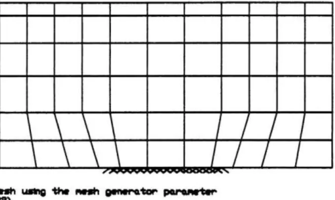
Using as unknowns the mesh generator parameters,
the optimal configuration is shown in Fig. 3. The
value of the total potential energy related to this
configuration is V= -48.22
J
.
In order to check the influence of the reduction of
the number of unknowns, the total number of node
coordinates have been used in the optimization
pro-cedure. The obtained optimal configuration is
rep-resented in Fig. 4. The total potential energy is
I
I
I
I
I I 1
Fig. 3. Example I. Optimal mesh using the mesh generator.
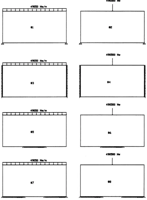
Table I. Total potential energy (Fig. 5) Case Uniform mesh Optimal mesh
I -210.72J -230.14J
2 -225.33J -255.141 3 -20.79J -27.66 J
4 -94.07 J -110.05 J
5 -40.22 J - 54.93 J 6 - 52.05} -58.97 J 7 -99.86 J - 115.88 J 8 -100.78 J -120.78 J
V = -54.93 J for this situation. From the figure it is observed that the node positions nearly follow the isostatic (principal stresses) lines.
490SO Nw/ft
11
13
17
Difference (%) Exact value (%)
9.21 15.56 13.23 16.54 33.04 18.05
16.98 17.09 36.57 15.79 13.29 17.35 16.04 13.50
19.84 17.99
Several different cases have been analysed in order to check the optimal mesh properties. They have been represented in Fig. 5. The results obtained for these
490500 Nw
I
490500 Nw
I
490500 Nw
l
16
490500 Nw
l
18
•90:50 Nw/1'1
~
-F1IW.. MESH <V •-7023 J> Fig. 6. Example 2.
cases are given in the table. Likewise the 'exact' values
of the total potential energy of each case have been
computed (using a FE analysis with more than 500
nodes) in order to assess the efficiency of these
optimal meshes.
Finally in Fig. 6, a more complicated example has
been studied. The initial mesh and the final mesh are
shown together with the values of the corresponding total potential energy.
RECOMMENDATIONS AND SUGGESTIONS
From a large number of analysed cases some
provisional recommendations about the design of FE
meshes can be concluded. First, the mesh should be more dense in the areas of discontinuities (geometric,
concentrated loads, large gradients of stresses, etc.).
Second, it may be interesting to try to adapt the node
positions along isostatic lines. This point is now
under investigation in order to check its general validity. The use of a different functional to the total potential energy as a measure of the goodness of a FE
mesh is currently being investigated.
REFERENCES
I. I. Babuska, The p and h-p versions of the finite element
method. The state of the art. Inst. Phys. Sci. and Tech. Note BN-1156, University of Maryland (1986). 2. I. Babuska, 0. C. Zienkiewicz, J. Gago and E. Oliveira,
Accuracy Estimates and Adaptive Refinement in Finite
Element Computation. John Wiley, Chichester (1986).
3. 0. C. Zienkiewicz and J. Z. Zhu, Error estimates and adaptivity. The essential ingredients of engineering FEM analysis. 2nd Conference on FEM, Stratford upon Avon, May (1989).
4. B. M. McNeice and P. V. Marcal, Optimization of finite element grid based on maximum potential energy. Tech-nical Report No. 7. University of Brown, Providence (1971).
5. D. J. Turcke and B. M. McNeice, Guidelines for selecting finite element grids based on an optimization study. Comput. Struct. 4, 499-519 (1974).
6. M. S. Shephard, R. H. Gallagher and J. F. Abet, The synthesis of near optimum Finite Element meshes with interactive computer graphics. lnt. J. Numer. Meth. Engng 15, 1021-1039 (1980).
7. A. Samartin, Un estudio sobre la exactitud del metodo de Ios Elementos Finitos. Aplicaci6n a la barra recta de secci6n variable bajo acciones axiles. Departamento de Analisis de !as Estructuras, ETSICCP, Santander (1980).