JHEP03(2018)153
Published for SISSA by SpringerReceived:December 27, 2017 Accepted: March 14, 2018 Published: March 26, 2018
FRW and domain walls in higher spin gravity
R. Aros,a C. Iazeolla,b J. Nore˜na,c E. Sezgin,d P. Sundella and Y. Yina a
Departamento de Ciencias F´ısicas, Universidad Andres Bello, Republica 220, Santiago de Chile, Chile
b
NSR Physics Department, G. Marconi University, via Plinio 44, Rome, Italy
c
Instituto de F´ısica, Pontificia Universidad Cat´olica de Valpara´ıso,
Casilla 4059, Valpara´ıso, Chile
d
Mitchell Institute for Fundamental Physics and Astronomy, Texas A&M University, College Station, TX 77843, U.S.A.
E-mail: [email protected],[email protected],[email protected],
[email protected],[email protected],[email protected]
Abstract:We present exact solutions to Vasiliev’s bosonic higher spin gravity equations
in four dimensions with positive and negative cosmological constant that admit an in-terpretation in terms of domain walls, quasi-instantons and Friedman-Robertson-Walker (FRW) backgrounds. Their isometry algebras are infinite dimensional higher-spin exten-sions of spacetime isometries generated by six Killing vectors. The solutions presented are obtained by using a method of holomorphic factorization in noncommutative twistor space and gauge functions. In interpreting the solutions in terms of Fronsdal-type fields in space-time, a field-dependent higher spin transformation is required, which is implemented at leading order. To this order, the scalar field solves Klein-Gordon equation with conformal mass in (A)dS4.We interpret the FRW solution with de Sitter asymptotics in the context
of inflationary cosmology and we expect that the domain wall and FRW solutions are as-sociated with spontaneously broken scaling symmetries in their holographic description. We observe that the factorization method provides a convenient framework for setting up a perturbation theory around the exact solutions, and we propose that the nonlinear com-pletion of particle excitations over FRW and domain wall solutions requires black hole-like states.
Keywords: Cosmology of Theories beyond the SM, Higher Spin Gravity, Higher Spin
Symmetry
JHEP03(2018)153
Contents1 Introduction 1
2 Bosonic Vasiliev model 5
2.1 Review of the full equations of motion 5
2.1.1 Non-commutative space 5
2.1.2 Master fields 6
2.1.3 Kinematic conditions 7
2.1.4 Equations of motion 7
2.1.5 Component form 8
2.1.6 Deformed oscillators 8
2.1.7 Discrete symmetries 9
2.1.8 Manifest Lorentz covariance 10
2.2 Vacuum solutions 10
2.3 Normal ordered perturbation scheme 12
2.4 Gauge function method 14
2.4.1 Topological field theory approach 14
2.4.2 Gauge functions 15
2.4.3 A universal particular solution in holomorphic gauge 17
3 Construction of the exact solutions with six symmetries 18
3.1 Initial data for Weyl zero-form with six Killing symmetries 18
3.1.1 Unbroken symmetries 18
3.1.2 Invariant Weyl-zero form integration constant 19
3.1.3 Regular presentation 19
3.1.4 Limits 21
3.1.5 Regularization of star products 21
3.2 Twistor space connection in holomorphic gauge 22
3.3 Master fields inL-gauge 24
3.3.1 Weyl zero-form 24
3.3.2 Twistor space connection at even orders 26
3.3.3 Twistor space connection at odd orders 26
3.3.4 Spacetime connection 27
3.3.5 Patching 27
3.4 Reaching Vasiliev gauge at first order 27
3.4.1 The Weyl zero-form 27
3.4.2 Twistor space connection 27
3.4.3 Spacetime connection 29
JHEP03(2018)153
4 Regularity of full master fields on correspondence space 304.1 Linearized scalar field profile 30
4.2 (Ir)regularity of Weyl zero-form 32
5 The iso(3) invariant solution and cosmology 34
5.1 The solution at linear order in deformation parameter 34
5.2 Comparison with standard cosmological backgrounds 35
5.3 Towards perturbation theory around exact solutions 37
6 Conclusions 39
A Conventions and definitions 41
B Coordinate systems and Killing vectors 42
B.1 Embedding space 42
B.2 Killing vector fields 42
B.3 GlobaldS4/S3 and AdS4/AdS3 foliations (iso-scalar leafs forǫk=−1) 43
B.4 Bifurcating (A)dS4/{dS3, H3} foliations (iso-scalar leafs for instantons) 44
B.5 Planar coordinates for (A)dS4 (iso-scalar leafs for ǫk= 0) 44
B.6 Stereographic coordinates 45
C Gauge functions 47
C.1 Stereographic coordinates 47
C.2 Stereographic coordinates for (A)dS4 47
C.3 Global foliation coordinates forǫk=−1 48
C.4 Planar coordinates for (ǫ, k) = (±1,0) 48
D Analysis of integrability condition on H(1)|Z=0 50
E Lemmas 51
E.1 A twistor space distribution 51
E.2 Fusion rules 52
1 Introduction
Vasiliev’s theory in four dimensions [1] has so far been studied mainly around its maximally symmetric anti-de Sitter vacuum. The perturbations around the anti-de Sitter spacetime describe an unbroken phase of the theory, with spectrum given by infinite towers of massless fields, corresponding to conserved higher spin currents of dual free conformal field theories in three dimensions [2–4]. Higher spin gravity is well known to admit a cosmological term of positive sign and de Sitter vacuum solution as well. It has been proposed that the parity invariant minimal version of higher spindS4 gravity is holographically dual to the three
JHEP03(2018)153
scalars residing at the boundary of dS4 at future timelike infinity [5]. For further
develop-ments in this direction, see [6–12]. These studies mostly exploit the higher spin symmetries. On the other hand, a detailed bulk description of the early universe physics, including the inflationary era, requires understanding of accelerating solutions of Vasiliev theory and cos-mological perturbations around them. Such solutions have isometries forming a subgroup of the de Sitter spacetime symmetries.
Higher spin gauge symmetries can be broken by quantum [13] as well as classical effects. In the latter case, a simple mechanism is to replace the maximally symmetric vacuum by vacua with six Killing symmetries forming a Lie algebra g6, as summarized
in table 1.1 These correspond to the isometries of domain walls, FRW-like solutions and quasi-instantons.2 While we shall leave to a future work an analysis of the the holographic aspects of the exact solutions that we present here, we propose to interpret the domain walls as bulk duals of vacua of three-dimensional massive quantum field theories arising through spontaneous breaking of conformal (higher spin) symmetries; for a relatively recent study of spontaneous breaking of scale invariance in certain CFTs in D= 3, see [16].
In this paper, we shall use a solution generating technique [17–19] to buildg6-invariant
solutions to Vasiliev’s bosonic theory with non-vanishing (positive or negative) cosmological constant from gauge functions, representing large gauge transformations that alter the asymptotics of the gauge fields, and g6-invariant scalar field profiles in the maximally
symmetric background. Solutions of Vasiliev’s equations with g3,g4 and g6 symmetries,
which are subgroups of theAdS4 symmetry group, were constructed only at the linearized
level in [14] (see [19] for a review) by using a different technique. The fully non-linear solutions presented in this paper are instead obtained by using a different method based on a holomorphic factorization ansatz, and in what we refer to as the holomorphic and
L-gauges, described in section 3. In furnishing an interpretation of the solution in terms of Fronsdal-type fields in spacetime, however, a higher spin transformation needs to be implemented order by order in weak fields to reach what we refer to as the Vasiliev gauge, also discussed in section3. We have implemented this gauge transformation only at leading order in this paper, leaving the computation of higher order terms to a future work. As we shall see in section 5, an important advantage of the method we have used to obtain the exact solutions in the holomorphic gauge is the validity of linear superposition principle in constructing solutions, thus facilitating the description of fluctuations around an exact solution. Even though we leave to future work the analysis of a cosmological perturbation theory around our solutions, an inspection of the star product algebra among the master field will lead us to propose that the nonlinear completion of particle excitations over FRW and domain wall solutions requires black hole-like states (see [18] for the study of scalar particle fluctuations over higher-spin black hole modes).
1The various vacua possess unbroken higher spin symmetries; the unbroken symmetry algebra of the
g6-invariant vacua is the intersection of the enveloping algebra ofg6 with the unbroken symmetry algebra of the maximally symmetric vacua (see [14] for the case of an so(1,3)-invariant solution), which is given by the quotient of the enveloping algebra of the (A)dS4 Killing symmetry algebra over the two-sided ideal given by the singleton annihilator.
2The quasi-instantons are Lorentzian counter parts of instantons, which can be viewed as the results of
JHEP03(2018)153
Among all solutions we have found, we shall, in particular, take a closer look at the FRW-like solution withiso(3) symmetry and positive cosmological constant. We will pro-vide a perturbative procedure for obtaining the solutions in the Vasiliev gauge mentioned above, to any order in a suitable perturbation parameter that breaks the de Sitter sym-metry to iso(3). On the solutions, the scalar field, whose value is vanishing in de Sitter vacuum, is turned on at first order in the symmetry-breaking parameter, and the metric gets corrected at the second order. Moreover, at linear order the fields with spins s > 2 vanish in the background solution. Whether they arise in higher orders remains to be de-termined. At linear order the scalar field behaves similarly to a conformally coupled scalar field in dS4. In section 5, we shall compare its behaviour with that of the inflaton in the
standard cosmological scenarios.
The FRW-like solutions are intriguing because if higher spin fluctuation fields are suppressed by the background, then they may yield cosmologically viable models based on Vasiliev’s theory, opening up a new window for embedding the standard models of particles and cosmology into higher spin theory, which may be viewed as the unbroken phase of string theory in which the string is tensionless [2,21–24]. This setting will inevitably involve the coupling of an infinite number of (massive) higher spin multiplets. One may envisage a scenario in which their presence will play a role in the resolution of the initial singularity, and near the end or after the inflation when the breaking of higher spin symmetry is expected to take place. A much bolder proposal would be the consideration of only massless higher spin theory with its matter couplings furnished through the Konstein-Vasiliev or supersymmetric extension of Vasiliev theory (see [26] for a survey). Such a proposal is motivated by the high degree of symmetry that may yield a UV finite theory, and by the availability of a mechanism [13] for breaking of higher spin symmetries by quantum effects without the need to introduce fields other than those present in the theory, whose spectrum consists of the two-fold product of the singleton representation of the AdS4
group. Thus it is natural to consider the (matter coupled) higher spin theory as the candidate for a tensionless limit of string theory, in which all the massive trajectories are decoupled completely, and to investigate its consequences for the early universe physics. There are very powerful no-go theorems that forbid accelerating spacetimes in string theory in its tensile phase (see [27] and references therein), inviting the considerations of non-perturbative and string loop effects in a full-fledged formulation of string field theory, and finding its vacuum solutions. On the other hand, higher spin theory can be viewed as a much simpler version of string field theory, in which finding asymptotically de Sitter vacua is a more amenable problem.
The introduction of matter and higher spin symmetry breaking remain a largely un-charted terrain. These aspects are expected to play key roles either for reheating in an inflationary scenario or an analogous mechanisms in non-inflationary scenarios. In the sim-plest inflation model in standard cosmology, Einstein gravity and a single real scalar field with a suitable potential dominate the early inflationary phase. Here we instead envisage a scenario in which the Einstein plus scalar system is replaced by the bosonic Vasiliev higher spin theory, which consists of a coupled set of massless fields with all integer spins
JHEP03(2018)153
rapidly inflated fluctuation modes with wavelengths larger than the Hubble length freeze and subsequently re-enter the cosmological horizon after inflation has ended. Assuming that higher spin symmetry breaking and reheating take place at around the same time, one can compute the effects of higher spin fluctuations on the CMB observations at large scales. In these scenarios, it is important to keep in mind that while the higher spin modes may dissipate in time, their couplings to and mixing with the gravitational field may have observable effects. Some studies have already been done along these lines, see e.g. [28–30], but based on assumptions on higher spin dynamics not born out of Vasiliev’s theory. Let us also note that the analog of theso(1,3) invariant solution, referred to as the “instanton” solution in table 1, was obtained as an exact solution for Λ< 0 in [15] and for Λ >0 as well in [20]. In the case of Λ < 0, a cosmological implications of the solution has been discussed in [15] where it has been argued that it leads to a bouncing cosmology, in some respects reminiscent of the work of [31] based on supergravity considerations.3
This paper is organized as follows: in section2, we review Vasiliev’s higher spin gravity equations. They are formulated in terms of master one-formAand master Weyl zero-form Φ which live on a base manifold X4 × Z4 with coordinates (xµ, Zα) where Z4 is a
non-commutative real four manifold. The master fields also depend on the coordinates of the fiber spaceY4 with coordinates Yα. In section3, we describe the construction of the exact
solutions with g6 symmetries. For the reader’s convenience we summarize the solutions
here. The master fields are the zero-form Φ and one-formAwhose components are displayed in (2.11). In holomorphic gauge, Φ′ is given in table 1, andA′α in (2.88) and (2.93). In the
L-gauge, Φ(L) is given in (3.53) and (3.12), A(L)
α is given in (3.54) and (3.61), and Wµ(L)
in (3.64). In Vasiliev gauge, the linear order results for Φ(G,1) is given in (3.66), A(αG,1)
in (3.78) and A(µG,1) is given by (A)dS connection with a detailed discussion of G-gauge
transformations given in3.4.3 and appendixD. In section 4, we examine the regularity of the Weyl zero-form. The scalar field profiles φ(x) are described in a unified manner by using stereographic coordinate system. In studying their regularity, one needs to distinguish between singularities that are gauge artifacts and genuine singularities in the full (x, Y, Z) space, sometimes referred to as the correspondence space. To this end, one needs to study the solution Φ(x, Y, Z) for the Weyl zero-form, and associated higher spin invariant and the on-shell conserved zero-form charges, as we shall discuss further in section4. In section5, we take a closer look at the iso(3) invariant solution and compare with the standard cosmological backgrounds. In section6, we summarize our results and comment on future directions. Frequently used symbols and notation are summarized in appendixA. Various coordinates systems used to describe (A)dS and the associated Killing vectors are given in appendix B. The gauge functions used in the construction of the exact solutions are described in appendixC. Details of the passage to Vasiliev gauge in leading order are given in appendixD, and useful formula in the description of twistor space distributions and the star products of relevant projector operators are provided in appendixE.
3An analogue Lorentz-invariant instanton solutions, with additional twisted sectors of the theory excited,
JHEP03(2018)153
2 Bosonic Vasiliev modelIn what follows, we review the basic properties of Vasiliev’s equations [35] and their classical solution spaces, including boundary conditions in spacetime and twistor space suitable for asymptotically (anti-)de Sitter solutions. For a recent review of the exact solutions see [19].
2.1 Review of the full equations of motion
2.1.1 Non-commutative space
Vasiliev’s theory is formulated in terms of horizontal forms on a non-commutative fibered space C with four-dimensional non-commutative symplectic fibers and eight-dimensional base manifold equipped with a non-commutative differential Poisson structure. On the total space, the differential form algebra Ω(C) is assumed to be equipped with an associative degree preserving product ⋆, a differential d, and an Hermitian conjugation operation †, that are assumed to be mutually compatible in the sense that iff, g, h∈Ω(C), then
(f ⋆ g)⋆ h=f ⋆(g ⋆ h), (2.1)
d(df) = 0, d(f ⋆ g) = (df)⋆ g+ (−1)|f|f ⋆(dg), (2.2) (df)†=d(f†), (f ⋆ g)†= (−1)|f||g|(g†)⋆(f†), (2.3)
where|f|denotes the form degree off. We shall also assume that4
(f†)†=f . (2.4)
It is furthermore assumed that Ω(C) contains a horizontal subalgebra, Ωhor(C), consisting
of equivalence classes defined using a globally defined closed and central hermitian top-form on the fiber space, and whose product, differential and hermitian conjugation operation we shall denote by ⋆,dand †as well.
The base manifold is assumed to be the direct product of a commuting real four-manifold X4 with coordinates xµ, and a non-commutative real four-manifold Z4 with
co-ordinates Zα; the fiber space and its coordinates are denoted by Y4 and Yα
′
, respectively. The non-commutative coordinates are assumed to obey
[Yα′, Yβ′]⋆ = 2iCα ′β′
, [Zα, Zβ]⋆=−2iCαβ, [Yα, Zβ ′
]⋆ = 0, (2.5)
and the differential Poisson structure is assumed to be trivial in the sense that
[Yα′, dYβ]⋆= [Zα, dYβ ′
]⋆ = [Zα, dZβ]⋆ = [Zα, dZβ]⋆ = 0 . (2.6)
The star product is defined in (A.1). The non-commutative space is furthermore assumed to have a compatible complex structure, such that
Yα′ = (yα′,y¯α˙′), Zα = (zα,z¯α˙), (2.7) (yα′)†= ¯yα˙′, (zα)†=−z¯α˙, (2.8)
4More generally,† ◦ †can be an automorphism of Ω(C), which is of relevance, for example, in the case
JHEP03(2018)153
where the complex doublets obey
[yα′, yβ′]⋆ = 2iǫα ′β′
, [zα, zβ]⋆ =−2iǫαβ . (2.9)
The horizontal forms can be represented as sets of locally defined forms onX4× Z4 valued
in oscillator algebrasA(Y4) generated by the fiber coordinates glued together by transition
functions. Assuming the latter to be defined locally on X4 yields a bundle over X4 with
fibers given by the differential graded associative algebra Ω(Z4)⊗ A(Y4), whose elements
can be given represented using symbols defined using various ordering schemes, which correspond to choosing different bases for the operator algebra. In what follows, we shall assume that it is possible to describe the field configurations using symbols defined in the Weyl ordered basis, which is manifestly Sp(4;R)×Sp(4;R)′ invariant, as well as the normal
ordered basis consisting of monomials in5
aα:=Yα+Zα, bα:=Yα−Zα, (2.10)
witha- andb-oscillators standing to the left and right, respectively, which breaks Sp(4;R)×
Sp(4;R)′ → (Sp(4;R)×Sp(4;R)′)diag. Equivalently, we shall assume that the elements in
Ω(Z4)⊗ A(Y4) have well-defined symbols in normal order, which can be composed using
the Fourier transformed twisted convolution formula (A.1), and that they can furthermore be expanded over the Weyl ordered basis of A(Y4) with coefficients in Ω(Z4), using the
aforementioned star product.
As for the fiber algebraA(Y4), it is assumed to be an associative algebra closed under
the star product and the hermitian conjugation operation † defined above. As we shall describe in more detail in sections 2.4 and 5.3, the algebra A(Y4) will furthermore be
assumed to contain certain nonpolynomial elements and distributions playing a role in constructing higher spin background and fluctuation fields.6
2.1.2 Master fields
The model is formulated in terms of a zero-form Φ, a one-form
A=dxµAµ+dzαAα+dz¯α˙Aα˙, (2.11)
and a non-dynamical holomorphic two-form
J :=−ib 4dz
α∧dz
ακ , (2.12)
with Hermitian conjugateJ = (J)†, where bis a complex parameter and
κ:=κy ⋆ κz, κy := 2πδ2(y), κz := 2πδ2(z), (2.13) 5The normal order reduces to Weyl order for elements that are independent of eitherY orZ.
6In order to construct higher spin invariants playing a role as classical observables, the algebra needs
JHEP03(2018)153
are inner Klein operators obeying
κy⋆ f ⋆ κy =πy(f), κz⋆ f ⋆ κz =πz(f), (2.14)
for any zero-formf, whereπy and πz are the automorphisms of Ω(Z4)⊗ A(Y4) defined in
Weyl order by
πy : (x;z,z¯;y,y¯)7→(x;z,z¯;−y,y¯), πz: (x;z,z¯;y,y¯)7→(x;−z,z¯;y,y¯), (2.15)
and πy◦d=d◦πy andπz◦d=d◦πz. It follows that
dJ= 0, J ⋆ f =π(f)⋆ J , π(J) =J , π:=πy◦πz, (2.16)
for any form f,idem J and ¯π :=πy¯◦πz¯.
2.1.3 Kinematic conditions
Higher spin gravities consisting of Lorentz tensor gauge fields can be obtained by imposing the integer-spin projection
π◦¯π(Φ) = Φ, π◦π¯(A) =A .
Models in Lorentzian spacetimes with cosmological constants Λ are obtained by imposing reality conditions as follows [20]:
ρ(Φ†) =π(Φ), ρ(A†) =−A , ρ:= (
π , Λ>0,
Id,Λ<0, (2.17)
that is, the real form of the sp(4;C) realized in terms of bilinears in Yα is chosen by the
Hermitian conjugation operation ρ◦ †; the consistency follows from ¯π(f) = (π(f†))† and the fact that if Λ > 0, then (ρ ◦ †)2 ≡ π ◦π¯, which reduces to the identity modulo the integer-spin projection.
2.1.4 Equations of motion
Introducing the curvature and twisted-adjoint covariant derivative defined by
F :=dA+A ⋆ A , DΦ :=dΦ + [A,Φ]π, (2.18)
respectively, one has the Bianchi identities
DF :=dF + [A, F]⋆ ≡0, DDΦ :=d(DΦ) + [A, DΦ]π ≡[F,Φ]π, (2.19)
where ordinary andπ-twisted star commutators
[f, g]⋆ :=f ⋆ g−(−1)|f||g|g ⋆ f , [f, g]π :=f ⋆ g−(−1)|f||g|g ⋆ π(f), (2.20)
respectively. The Vasiliev equations of motion are given by
JHEP03(2018)153
which are compatible with the kinematic conditions and the Bianchi identities, implying that the classical solution space is invariant under the following infinitesimal gauge trans-formations:
δA=Dǫ:=dǫ+ [A, ǫ]⋆, δΦ =−[ǫ,Φ]π, (2.22)
for parameters obeying the same kinematic conditions as the connection, viz.
ππ¯(ǫ) =ǫ , ρ(ǫ†) =−ǫ . (2.23)
2.1.5 Component form
Decomposition of the equations of motion under the coordinate basis (∂~µ, ~∂α) for the
tan-gent space of the base manifold, yields the Vasiliev equations
Fµν = 0, DµΦ = 0, Fµα = 0, DαΦ = 0, (2.24)
Fαβ+ ib
2 Φ⋆ κǫαβ = 0, Fαβ˙= 0, Fα˙β˙+ i¯b
2 Φ⋆κǫ¯ α˙β˙ = 0, (2.25) DµΦ =ı∂µ~ DΦ =∂µΦ +Aµ⋆Φ−Φ⋆ π(Aµ), (2.26) DαΦ =ı∂α~ DΦ =∂αΦ +Aα⋆Φ−Φ⋆π¯(Aα), (2.27) Dα˙Φ =ı∂~α˙DΦ =∂α˙Φ +Aα˙ ⋆Φ−Φ⋆ π(Aα˙), (2.28)
usingπ(A) = ¯π(A), ¯π(dzα) = dzα and π(dz¯α˙) =dz¯α˙, and the one-form components obey
the following kinematic conditions:
ππ¯(Aµ, Aα, Aα˙) = (Aµ,−Aα,−Aα˙), (2.29)
(Aµ, Aα, Aα˙)† =
(
(−π(Aµ), π(Aα˙),π¯(Aα)), Λ>0,
(−Aµ, Aα˙, Aα), Λ<0.
(2.30)
2.1.6 Deformed oscillators
Alternatively, introducing
Sα:=zα−2iAα, Sα˙ =zα˙−2iAα˙, (2.31)
the equations of motion involving twistor-space derivatives can be written as
DµSα = 0, DµSα˙ = 0, (2.32)
[Sα, Sβ]⋆ =−2iǫαβ(1−bΦ⋆ κ), [Sα, Sβ˙]⋆ = 0, [Sα˙, Sβ˙]⋆ =−2iǫα˙β˙(1−¯bΦ⋆κ¯),
(2.33)
Sα⋆Φ+Φ⋆ π(Sα) = 0, Sα˙ ⋆Φ + Φ⋆¯π(Sα˙) = 0, (2.34)
that is, the master fields (Sα, Sα˙) define a covariantly constant set of Wigner-deformed
JHEP03(2018)153
conditions and integer-spin conditions as follows:
ππ¯(Sα, Sα˙) = (−Sα,−Sα˙), (2.35)
(Sα, Sα˙)† =
(
(−Sα˙,−Sα) for Λ<0,
(−π(Sα˙),−π¯(Sα)) for Λ>0 .
(2.36)
Besides being useful in constructing exact solutions, observables and exhibiting certain dis-crete symmetries, the deformed oscillators facilitate the casting of the equations of motion into a manifestly Lorentz covariant form.
2.1.7 Discrete symmetries
The equations of motion and the gauge transformations exhibit the following discrete sym-metries:
i) Holomorphic parity transformation
(Φ, A;ǫ)7→(π(Φ), π(A);π(ǫ)) ; (2.37)
ii) Deformed oscillator parity transformation
(Φ, Aµ, Sα;ǫ)7→(Φ, Aµ,−Sα;ǫ), (2.38)
which is equivalent to Aα 7→ −iZα−Aα;
iii) Vectorial parity transformation
(Φ, A;ǫ)7→(P(Φ), P(A);P(ǫ)), (2.39)
whereP is the star product algebra automorphism
P(yα,y¯α˙;zα,z¯α˙) := (¯yα˙, yα; ¯zα˙, zα), d◦P :=P ◦d , (2.40)
from which it follows that P◦ †=† ◦P and P◦π = ¯π◦P.
From
P(J) =−(b/¯b)J , (2.41) it follows that (iii) exchanges a solution to the equations with parameterbto a solution to the equations with parameter ¯b. In particular, if ¯b=±b, then one can extendP to
b
P =P◦P′, (2.42)
whereP′is an internal parity map acting on the component fields, and project the spectrum of the theory by demanding
b
P(A,Φ) = (
(A,Φ) b= 1 (A model),
(A,−Φ) b=i (B model), (2.43)
JHEP03(2018)153
2.1.8 Manifest Lorentz covarianceTo cast the equations on a manifestly Lorentz covariant form, one introduces the field-dependent generators [35,36]
Mαβ(tot):=y(α⋆yβ)−z(α⋆zβ)+S(α⋆Sβ), Mα(tot)˙β˙ := ¯y( ˙α⋆y¯β˙)−z¯( ˙α⋆z¯β˙)+S( ˙α⋆Sβ˙), (2.44)
and redefines
Aµ=Wµ+
1 4i
ωµαβMαβ(tot)+ωµα˙β˙M(tot)
˙ αβ˙
, (2.45)
where (ωµαβ(x), ωα˙ ˙ β
µ (x)) is a bona fide canonical Lorentz connection on X4, after which
the equations of motion involving spacetime derivatives can be re-written on the following manifestly Lorentz covariant form7 [17,37,38]:
∇W +W ⋆ W+ 1 4i
rαβMαβ(tot)+rα˙β˙M(tot)
˙ αβ˙
= 0, (2.46)
∇Φ +W ⋆Φ−Φ⋆ π(W) = 0, ∇Sα+ [W, Sα]⋆ = 0, (2.47)
where
∇W :=dW + [ω(0), W]⋆, ∇Φ :=dΦ + [ω(0),Φ]⋆, (2.48) ∇Sα:=dSα−ωαβSβ+ [ω(0), Sα]⋆, (2.49) rαβ :=dωαβ−ωαγ∧ωγβ, rα˙β˙:=dωα˙β˙−ωα˙γ˙ ∧ωγ˙β˙, (2.50)
with
ω(0) := 1 4i
ωαβMαβ(0)+ωα˙β˙M(0)
˙ αβ˙
, (2.51)
Mαβ(0) := y(α⋆ yβ)−z(α⋆ zβ), M(0)
˙
αβ˙ := ¯y( ˙α⋆y¯β˙)−z¯( ˙α⋆z¯β˙) . (2.52)
The Lorentz connection is defined, as usual, up to tensorial shifts, that can be fixed by requiring that the projection of W onto Mαβ(0) vanish atZ = 0.
2.2 Vacuum solutions
Flat connections. The equations of motion admit solutions
Φ = 0, A= Ω, (2.53)
where Ω is a locally defined one-form onX4× Z4 valued in A(Y4) that is flat, viz.
dΩ + Ω⋆Ω = 0 . (2.54)
If Ω∈Ω(X4)⊗ A(Y4), then there exists locally defined gauge functions Lon X4 such that
Ω =L−1⋆ dL , (2.55)
JHEP03(2018)153
that we shall refer to as vacuum connections, as they preserve higher symmetries with rigid parameters
ǫ=L−1⋆ ǫ′⋆ L , dǫ′ = 0, ǫ′ ∈ A(Y4) ; (2.56)
the space Ω(Z4)⊗ A(Y4), on the other hand, contains flat connections constructed from
projector algebras that cannot be described using gauge functions and that break some of the vacuum symmetries [14].
Maximally symmetric spaces. The (A)dS4 vacua are described by gauge functions
valued in the real formG10 of Sp(4;C) selected by the reality condition introduced above.
Thus,G10refers to AdS group for λ2>0 anddS group forλ2<0, with the commutation
rules for theg10 algebra given by
[MAB, MCD] = 4iη[C|[BMA]|D], ηAB := ηab,−sign(λ2) , ηab = diag(−+ ++) .
(2.57) and they can be realized in terms of theY-oscillators as
−ℓ−1Ma5 ≡Pa= λ
4 (σa)αβ˙y
αy¯β˙ , M ab=−
1 8
h
(σab)αβyαyβ+ (¯σab)α˙β˙y¯α˙y¯ ˙
βi, (2.58)
where
λ= (
ℓ−1 for Λ<0
iℓ−1 for Λ>0, (2.59)
It follows that
[Mab, Mcd]⋆ =iηbcMad+ 3 more, [Mab, Pc]⋆ = 2iηc[bPa], (2.60)
[Pa, Pb]⋆ =iλ2Mab (2.61)
with reality conditions
ρ((Pa)†) =Pa, ρ((Mab)†) = (Mab)†=Mab . (2.62)
Introducing coset elements
L:G10/SO(1,3) →G10, ρ(L†) =L−1, (2.63)
the Maurer-Cartan form decomposes into a frame field and a Lorentz connection as follows:
Ω = 1 4iΩαβY
αYβ = 1
4i
2Ωαα˙yαy¯α˙ + Ωαβyαyβ+ Ωα˙β˙y¯α˙y¯ ˙ β=iΩ
aPa+ 1
2iΩabM
ab (2.64)
where thus
Ωαα˙ =−
λ
2(σa)αα˙Ω
a, Ω
αβ :=−
1
4(σab)αβΩ
ab, Ω ˙ αβ˙ =−
1
4(¯σab)α˙β˙Ω
ab . (2.65)
In these bases, the flatness condition reads
JHEP03(2018)153
that is
dΩαα˙ −Ωαβ∧Ωβα˙−Ωα˙β˙∧Ωαβ˙ = 0, (2.67)
Rαβ−Ωαα˙ ∧Ωαβ˙ = 0, Rα˙β˙−Ωα˙α∧Ωαβ˙ = 0, (2.68)
or
dΩa+ Ωab∧Ωb = 0, Rab+λ2Ωa∧Ωb = 0, (2.69)
where the Riemann two-form
Rαβ :=dΩαβ−Ωαγ∧Ωγβ =−
1 4(σab)
αβRab,
Rα˙β˙ :=dΩα˙β˙−Ωα˙γ˙ ∧Ωγ˙ ˙ β =−1
4(¯σab)
˙
αβ˙Rab, (2.70)
withRab:=dΩab+ ΩacΩcb.
The full equations of motion can be solved in two dual fashions, one involving nor-mal ordered scheme and perturbatively defined Fronsdal fields, and the other based on a topological field theory approach, which we describe below.
2.3 Normal ordered perturbation scheme
In the normal order, defined by the star product formula (A.1), the inner Klein operators become real analytic in Y andZ space,viz.
κ=κy ⋆ κz= exp(iyαzα), κ¯=κy¯⋆ κ¯z = exp(iy¯α˙z¯α˙) . (2.71)
Assuming that the full field configurations are real-analytic onZ4 for generic points inX4,
one may thus impose initial conditions
Φ|Z=0=C , Aµ|Z=0=aµ . (2.72)
Assuming furthermore thatAα|C=0 is a trivial flat connection onZ4, that one may choose
to beAα|C=0 = 0, and choosing a homotopy contractor for the de Rham differential onZ4,
which entails imposing a gauge condition on Aα, one may solve the constraints on DαΦ, Fαβ and Fαµ on Z4 in a perturbative expansion of the form:
Φ =X
n>1
Φ(n)(C, . . . , C), Φ(1)(C)≡C ,
Aα =
X
n>1
A(αn)(C, . . . , C),
Aµ=
X
n>0
A(n)(aµ;C, . . . , C), A(0)(aµ)≡aµ, (2.73)
where Φ(n)(C, . . . , C) is an n-linear functional in C idem A(αn)(C, . . . , C) and A(n)(aµ;C, . . . , C), and the latter is linear in aµ. These quantities are real-analytic in Y4× Z4 provided that C and aµ are real analytic inY-space and all star products arising
JHEP03(2018)153
From the Bianchi identities, it follows that the remaining equations, that is, Fµν = 0
andDµΦ = 0, are perturbatively equivalent to Fµν|Z=0= 0 andDµΦ|Z=0= 0, which form
a perturbatively defined Cartan integrable system on X4 forC and aµ.
To Lorentz covariantize, one imposes
W|Z=0 =w , (2.74)
and DµΦ|Z=0 depend on the Lorentz connection only via the Lorentz covariant derivative ∇and the Riemann two-form (rαβ, rα˙β˙); it follows that
Perturbatively defined Fronsdal fields. Expanding the differential algebra around the (anti-)de Sitter vacuum
Φ(0) = 0, A(0) = Ω, (2.78)
and assuming that the homotopy contraction inZ-space is performed such that
zαA(1)α = 0, (2.79)
referred to as the Vasiliev gauge [40], the resulting linearized system on X-space provides an unfolded description of a dynamical scalar field
φ= Φ|Y=0=Z, (2.80)
and a tower of spin-s Fronsdal fields
φa(s) = ((e−1)µa)(0)
where we use the convention that repeated indices are symmetrized.
At the nonlinear level, the Cartan integrable system onX-space provides a deformation of the equations of motion for these fields, which is consistent as a set of partial differential equations but that depends on the choice of initial data for Φ andWµas well as the gauge
JHEP03(2018)153
choice that yields a formulation of higher spin gravity in X-space that lends itself to a standard path integral formulation remains an open problem.8
2.4 Gauge function method
2.4.1 Topological field theory approach
Alternatively, one may treat the system as an infinite set of topological fields on X4× Z4
packaged into master fields valued in A(Y4) represented by symbols in Weyl order, that is,
as expansions in terms of the generators of A(Y4) star multiplied by differential forms on
Ω(X4× Z4), referred to as mode forms.
The field configurations are assigned a bundle structure, whereby a projection ofA is assumed to define a connection valued in a Lie subalgebra ofA(Y4). The complementary
projection ofA, referred to as the generalized frame field, together with the Weyl zero-form Φ are taken to belong to adjoint and twisted adjoint sections, respectively, over X4× Z4,
which is treated as a base manifold; the two-forms J and J by their definition belong to twisted adjoint sections. The bundle connection is assumed to act faithfully on the sections, and the bundle curvature is assumed to be an adjoint section, as required by the equations of motion.
As for boundary conditions, the base manifold is assumed to be compact, and the sections, i.e. their mode forms, are assumed to be bounded away from a set of marked points representing boundaries. In a generic coordinate chart U ⊂ X4, the sections are
described by an integration constant for the Weyl zero-form, a flat connection on Z4 and
a gauge function on U × Z4. At the marked points, the initial data instead consists of
prescribed singularities in the generalized frame field and related fall-off in the Weyl zero-form (including the physical scalar field). For asymptotically (anti-)de Sitter solutions, we take X4 to have the topology of S1×S3 with a marked S1, such that, to all orders in
classical perturbation theory, the leading terms in the master fields at the markedS1× Z 4
describe a set of free Fronsdal fields, which one may view as a condition at the boundary of (A)dS4 times Z4. To impose boundary conditions on Z4, we assume that Ω(Z4)
i) is closed under star products, which can be achieved by taking the Fourier transforms of the zero-forms in Ω(Z4) to be L1 in momentum space (i.e. to be expandable in
terms of plane waves that generate a twisted abelian group algebra), which requires the zero-form sections onZ4 to be bounded atZ = 0;
ii) has a graded trace operation given by integration of the top-forms on Z4, which
requires these to fall off atZ =∞ so as to belong to L1(Z 4).
Finally, A(Y4) is taken to be a set of operators in a quantum-mechanical system equipped
with a (possibly regularized) trace operation that is dual to the boundary conditions at the markedS1.
8To our best understanding, the standard classical Noether procedure breaks down [42], while there
JHEP03(2018)153
The above geometries can be characterized by functionals, playing the role of clas-sical observables (including on-shell actions), given by combined traces over A(Y4) and
integrations overX4× Z4 (possibly with insertions of delta functions localized to
subman-ifolds). These gauge transformations that leave these functionals invariant are referred to as proper, or small, gauge transformations, as opposed to large gauge transformations that alter the asymptotics of the fields and hence the value of the observables. The resulting moduli space is thus sliced into (proper) gauge orbits labelled by the observables, each of which defines a microstate of the theory.9
2.4.2 Gauge functions
In the topological field theory approach, solution spaces are obtained starting from a refer-ence solution (Φ′, A′)∈Ω({p0} × Z4)⊗ A(Y4) at a base pointp0 ∈ X4, constructed from an
integration constant C′ for Φ′ at, say, Z = 0, and an flat connection on Z
4, that we shall
trivialize in most of what follows. Moduli associated to the connection and generalized frame field onX4 are then introduced by means of a large gauge transformation
A(G)=G−1⋆(A′+d)⋆ G , Φ(G)=G−1⋆Φ′⋆ π(G), G=L ⋆ H , (2.82)
whereLis the vacuum gauge function, andHis a gauge function determined perturbatively by the requirements that
a) in Weyl order, Φ(G) and the twisted open Wilson lines V(M) := exp⋆(iMαSα(G)),
whereMα ∈C4 (for details, see [37, 38,46]), are sections in Ω(X
4× Z4)⊗ A(Y4) in
form degree zero; and
b) in normal order, (Φ(G), A(αG), Wµ(G)) asymptote to configurations describing free
Frons-dal fields10 in accordance with the central on mass-shell theorem close to the marked
S1× Z 4.
We shall refer refer to(a)and(b)as dual boundary conditions, as(a)requires factorization of the master fields in Weyl order, whereas(b) requires normal order. We thus propose to fixH(n) by requiring
i ) Manifest Lorentz covariance and real analyticity inY of the normal ordered symbols of (Φ(G), A(G)) at the origin ofY4×Z4, so that the field configurations are expandable
in terms of Lorentz tensorial component fields on X4 defined by Taylor expansion in
Y atY = 0 =Z.
9A subset of the classical observables are extensive; keeping these fixed defines a higher spin ensemble consisting of a large number of microstates. In [38,45], it has been proposed that the extensive variables are the zero-form charges [14,37], and in [46] it has been proposed that a complete set of classical observables in the case thatX4 has trivial topology is given by the space of twisted open Wilson lines inZ4. According to these proposals, the rigid symmetries of the vacuum should leave the extensive variables invariant while acting nontrivially on the microscopic variables; for related remarks, see [18,46].
10The full field configurations are thus assumed to contain contain asymptotically (anti-)de Sitter regions
JHEP03(2018)153
ii) the Weyl ordered symbols of (Φ(G), V(M)) to be traceable over Ω(Z4)⊗ A(Y4), for
there to exist higher spin invariants playing the role of classical observables;
iii) Perturbatively stable asymptotic Fronsdal fields in weak-coupling regions of X4
(where the Weyl zero-form goes to zero), for the classical observables to admit per-turbative expansions in terms of parameters related to sources for weakly coupled higher spin gauge fields.
The following additional remarks are in order:
1. Zig-zagging self-consistency: at nth order, the quantity Φ(G,n) is a functional of
H(n′)
with 1 6 n′ 6 n−1 and initial data C′(n′)
with 1 6 n′ 6 n, which means that condition (a), which must hold for finiteZ, is in effect a non-trivial admissibility condition on the Y-dependence of the initial dataC′, i.e. onA(Y4).
2. Residual small gauge transformations: the above conditions do not determine the hs1(4) part ofH(n), which is real analytic inY, and which can thus be used for small
gauge transformations inside the bulk.
3. Deformed oscillators: although the master fieldsS(G)are not sections, one can require
that Φ(G) and the twisted open Wilson loops V(M)) form an associative algebra with traces, which can be use to construct a complete set of higher spin invariant observables that one may think of as substitutes for the standard ADM-like charges that can be used to define higher spin ensembles in unbroken phases; for further details, see [18].
4. Residual symmetries: the full solution (Φ(G), A(G)) is left invariant under gauge
trans-formations with parameters
ǫ(G)=G−1⋆ ǫ′⋆ G , (2.83)
whereǫ′ are constant parameters stabilizing Ψ,viz.
[ǫ′,Ψ]⋆ = 0 . (2.84)
Conversely, given a set of symmetries forming a Lie algebra g, spaces of g-invariant solutions can be found by solving the linear constraint (2.84) on Ψ together with the conditions that Ψ belongs to an associative algebra that is left invariant under star multiplication by the inner Klein operators, i.e. Ψ⋆ κy and Ψ⋆Ψ should belong to
the algebra, which is the approach that we shall employ.
In summary, the dual boundary conditions are physically well-motivated and non-trivial; in this paper, we shall focus on their implementation at the linearized level, leaving higher orders, starting with the issue of whether Φ(G,2) obeys (a), for a forthcoming
JHEP03(2018)153
2.4.3 A universal particular solution in holomorphic gaugeFor all vector fields ~v tangent to X-space, we have ı~vA′ = 0, and hence ı
~vdA′ = 0 and ı~vdΦ′ = 0, i.e.
A′ =dzαA′α+dz¯α˙Aα′˙, ∂µΦ′= 0 =∂µA′α, (2.85)
and
Fαβ′ +ib 2 Φ
′⋆ κǫ
αβ = 0, Fα′β˙ = 0, (2.86)
∂αΦ′+A′α⋆Φ′−Φ′⋆π¯(A′α) = 0 . (2.87)
Thus, prior to switching on the gauge function G, we need to find a particular solution to the above system subject to a generic zero-form initial datum. To this end, we observe that the Ansatz11
Φ′ = Ψ(y,y¯)⋆ κy, A′α =A′α(z; Ψ) =
X
n>1
a(αn)(z)⋆Ψ⋆n, (2.88)
where thus both Ψ and Ψ⋆ κy are assumed to be elements in A(Y4), and
Ψ†=ρ(Ψ)⋆ κyκ¯y¯, (2.89)
solves the fully non-linear equations provided that
πz(a(αn)(z)) =−a(αn)(z), (2.90)
and that
sα:=zα−2iaα, aα :=
X
n>1
a(αn)(z)νn, (2.91)
obeys the deformed oscillator algebra
[sα, sβ]⋆=−2iǫαβ(1−bνκz), κz⋆ sα =−sα⋆ κz . (2.92)
One class of solutions is given by [17]12
aα =− ibν
2 zα Z +1
−1
dτ
(τ+ 1)2 exp
iτ −1
τ + 1z
+z−
1F1(12; 2;bνlogτ2), (2.93)
where we have introduced a spin frame (u+α, u−α) obeying
u+αu−α = 1, (2.94)
11Note that this ansatz for A′
α is holomorphic inz, and hence the terminology of holomorphic gauge; see [19] for a review.
12As is well-known, upon representing Wigner’s deformed oscillatorss
αin a Fock space for the undeformed oscillatorszα, singular vectors appear for an infinite number of discrete critical values ofbν; for a brief review and references to original works, see [19]. It would be interesting to study the behaviour of the master fields close to these critical points, which we leave for a future study. In what follows, we shall assume thatbν
JHEP03(2018)153
and z± is defined in (A.4). The introduction of this frame is required in order to integrate the delta function in Weyl order without choosing any specific basis for Ψ(Y).
It is worth noting that, in the holomorphic gauge, the separation of the dependence on
Y andZ of the twistor space connectionAα leads to a non-analyticz-dependent coefficient aα(z), as given in eq. (2.93). Indeed, the separated deformed oscillator problem on Y × Z
reduces to one onZonly, with oscillatorssα(z), as given in eq. (2.92), deformed by the delta
function κz. As a consequence, the perturbative expansion of aα starts with an abelian
connection in two dimensions given by a distribution in Z whose curl is proportional to
κz. In the holomorphic gauge, it is given by eq. (2.93) with the hypergeometric function
replaced by a constant; the resulting distribution is discussed in appendixE. On the other hand, as we shall show later, once the star products betweenaα, the zero-form initial data
Ψ(Y) and the gauge function G = L ⋆ H are performed (in normal order), the resulting form of Aα is real analytic on Z already in the intermediate L-gauge to all orders in
perturbation theory, and on Y × Z for generic spacetime points in the Vasiliev gauge at first order in perturbation theory. Thus, in the latter gauge, we recover the standard generating functions for gauge fields and Weyl tensors, at least at the linearized level. The issue of what constitutes a physically meaningful gauge at higher orders will be discussed in the Conclusions, and left for future work.
Thus, in order to construct solution spaces with desired physical properties, we need to expand Ψ over suitable subalgebras ofA(Y4); for the cases of particle fluctuation modes
and black hole-like generalized Type D modes, see [17, 18]. In what follows, we shall examine a new type of subalgebras related to solutions with six Killing symmetries inside the isometry algebra of (A)dS4.
3 Construction of the exact solutions with six symmetries
In this section, we shall begin by describing the factorization method that will be used to construct the solutions. We shall than construct domain walls (DW), instantons13 (I) and FRW-like solutions (FRW) given by foliations of a four-dimensional spacetime M4 with
three-dimensional foliates M3 that are maximally symmetric metric spaces, we shall first
choose embeddings of the corresponding six-dimensional isometry algebrasg6 into the
ten-dimensional isometry algebra g10 of the vacuum solution. We then switch on g6-invariant
Weyl zero-forms and gauge functions.
3.1 Initial data for Weyl zero-form with six Killing symmetries
3.1.1 Unbroken symmetries
In order to describe foliations with maximally symmetric foliates, we embedg6 intog10as
follows [14]:
Mrs =LraLsbMab, Tr =Lra
αMabLb+βPa
, (3.1)
13The instantons break all transvection isometries of the vacuum solution, i.e.
JHEP03(2018)153
where14
α, β∈R, α, β >0, (α, β)6= (0,0), (3.2)
and the representatives of the cosetsso(3,1)/so(2,1) forǫ= 1, and the cosetso(3,1)/so(3) forǫ=−1 obey
LraLsbηab=ηrs, LaLa=ǫ , LraLa= 0, ηab= diag(−+ ++), ηrs = diag(++,−ǫ), ǫ=±1
(3.3)
where we have introduced the parameter ǫ. The resulting symmetry algebra reads as follows:15
[Mrs, Mpq] =iηspMrq+ 3 more, [Mrs, Tp] = 2iηp[sTr], (3.4)
[Tr, Ts] =−i(ǫα2−λ2β2)Mrs, (3.5)
giving rise to the cases listed in table 1.
3.1.2 Invariant Weyl-zero form integration constant
Imposingg6-invariance of zero-form initial data, viz.
[Mrs,Φ′]π = 0, [Tr,Φ′]π = 0, (3.6)
it follows from the first condition that
Φ′= Φ′(P), P :=LaPa,
and from the second condition that
−ǫβλ 2
8
d2
dP2 +iǫα
d dP + 2β
Φ′(P) = 0 . (3.7)
where we have used
LraLb[Mab, Pn]⋆ = inǫLraPaPn−1, (3.8)
Lra{Pa, Pn}⋆ = LraPa
2Pn−n(n−1)ǫλ
2
8 P
n−2
. (3.9)
3.1.3 Regular presentation
To solve (3.7), we Laplace transform Φ′ as
Φ′ = I
C dη
2πiΦe
′(η) exp(−4ηλ−1P)≡ Oexp(−4ηλ−1P). (3.10)
This gives a characteristic equation for η solved by
η±=−γ± p
ǫ+γ2 , γ := iα
λβ , η+η− =−ǫ , (3.11) 14One can always choose α > 0 by redefining La
r, after which one may take β > 0 using the global
Z2-symmetry generated by theπ-map, which exchangesβwith−β.
15The symmetry of the full solutions is generated by the parameters given by the conjugation of the
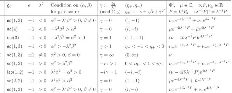
Type M3 g6 ǫ λ2 Condition on (α, β) γ := λβiα (η+, η−) Φ′, µ∈C, ν,ν, ν˜ ±∈R
forg6 closure (mod G10) η± ≡ −γ±
p
ǫ+γ2 P=La
Pa, (λ−1P)† =λ−1P
DW(dS)+ dS3 so(1,3) +1 <0 α2−λ2β2 >0,β 6= 0 γ = 0 (1,−1) ν+e−4λ
−1P
+ν−e4λ
−1P
FRW+ S3 so(4) −1 <0 −λ2β2 > α2 γ = 0 (i,−i) µe−4iλ
−1P
+ ¯µe4iλ−1P
FRW0 Eucl3 iso(3) −1 <0 −λ2β2 =α2 >0 γ = 1 (−1,−1) (ν−4˜νλ−1P)e4λ
−1P
FRW(dS)− H3 so(1,3) −1 <0 α2 >−λ2β2 γ >1 η−<−1< η+<0 ν+e−4η+λ
−1P
+ν−e−4η−λ
−1P
I dS3,H3 so(1,3) ±1 6= 0 α2 >0, β= 0 γ =∞ (0,∞) ν
DW(AdS)+ dS3 so(1,3) +1 >0 α2 > λ2β2 −iγ >1 0< iη−<1< iη+ ν+e−4η+λ
−1P
+ν−e−4η−λ
−1P
DW0 M ink3 iso(1,2) +1 >0 λ2β2=α2 >0 −iγ = 1 (−i,−i) (ν−4iνλ˜ −1P)e4iλ
−1P
DW− AdS3 so(2,2) +1 >0 λ2β2> α2 γ = 0 (1,−1) µe−4λ
−1P
+ ¯µe4λ−1P
FRW(AdS)− H3 so(1,3) −1 >0 α2+λ2β2 >0,β 6= 0 γ = 0 (i,−i) ν+e−4iλ
−1P
+ν−e4iλ
−1P
Table 1. g6-invariantM3-foliations arising in the bosonic models, with I standing for instantons, and FRWk and DWk, respectively, standing for
FRW-like solutions (ǫ=−1) and domainwalls (ǫ= +1) with foliates with curvatures of signk= sign(ǫα2 −λ2
β2
). The embeddings ofg6 into the isometry algebra of the (A)dS4 vacua are governed by a vectorL
a
withL2
=ǫ and two real parametersα, β >0. The last column contains the corresponding g6-invariant initial data for the Weyl zero-form. Two families of foliations with k =−1 interpolate between the cases with k= 0 and the instantons.
–
20
JHEP03(2018)153
that are either real or purely imaginary. Thus, forβ >0 we have
so(1,3) : Φe′(η) = ν+
η−η+
+ ν−
η−η−
, (3.12a)
iso(1,2), iso(3) : Φe′(η) = ν
η+√−ǫ + √
−ǫeν
(η+√−ǫ)2, (3.12b)
so(4), so(2,2) : Φe′(η) = µ
η−η+
+ µ¯
η−η−
. (3.12c)
The small contoursCencircle the poles ofΦe′counterclockwise. The corresponding solutions for Φ′ are listed in table1modulo rigidG10transformations, that can be used to setα = 0
for ǫk =−1 and sign(ǫΛ) = +1, i.e. the FRW+, the DW−, the the DW+ in dS4 and the
FRW− inAdS4.
3.1.4 Limits
The flat solutions withk= 0 arise from theso(1,3)-invariant families in the limit
γ →√−ǫ , (3.13)
keeping
ν :=ν++ν−, eν:=
γ−pγ2+ǫ −√−ǫ √
−ǫ (ν−−ν+), (3.14)
fixed. In the limit β→0, one has η+→0 andη− → ∞, and hence
e Φ′ = ν
η , ν≡ν+, (3.15)
and C is a small contour encirclingη = 0 counterclockwise.16
3.1.5 Regularization of star products
In order to compute
Ψ⋆Ψ = Φ′⋆ π(Φ′), (3.16)
we use the lemma
e−4ηλ−1P ⋆ e−4η′λ−1P = 1
(1−ǫηη′)2exp
−4 η+η ′
1−ǫηη′λ
−1P , (3.17)
and the regularization procedure spelled out in [17], viz.
e−4sλ−1P ⋆ e4sǫλ−1P|reg =
I
s dη
2πi(η−s)e
−4ηλ−1P
⋆ e4ǫsλ−1P
= I
s
dη
2πi(η−s)3 exp
4ηs−ǫ
η−sλ
−1P
= 0, (3.18)
16Alternatively, the decoupling of theη
+-mode in the limitβ→0 can be achieved using a twisted-adjoint
JHEP03(2018)153
whereC2 is a constant given by
ǫk=−1 : C2 = µ
where the last case contains the instantons, for which C2 =ν2.
3.2 Twistor space connection in holomorphic gauge
The general solution in integral form. In the expression for the twistor space connec-tion, it is convenient to express the hypergeometric function in an integral representation as follows
17Crucial for the regularization is that, after evaluating (any) one of the two integrals, the exponential
JHEP03(2018)153
Thus, expanding in powers of the deformation parameters, we find that all odd terms are linear in Ψ, while all even terms are (yα,y¯α˙)-independent,viz.
Let us proceed by looking into the internal connection order by order in its perturbative expansion.
First order. The linearized twistor space connection is given by
A′α(1) =a(1)α (z)⋆Ψ (3.30) For its basic distributional properties, see remark made above. Clearly, in Weyl order, the linearized twistor space connection is not real-analytic at the origin ofZ-space; whether it becomes real analytic in normal order depends on the details of Ψ, as we shall analyze in more detail below.
Second order. We have the second order
A′α(2)=−ib
Thus we can split the integral into two pieces as follows:
JHEP03(2018)153
which is convergent for all real w. Forw >0, we can integrate by parts and rewrite it as
I2>(w) =−e
w
wE1(w), (3.35)
where the exponential integral
E1(w) =
Z ∞
w dt
t e
−t, w >0 . (3.36)
This function can be extended from the positive real axis to a complex function that is analytic away from the negative real axis, where is has a Taylor expansion given by
E1(w) =−γE −logw−
∞ X
p=1
(−w)p
pp! , (3.37)
whereγE is the Euler-Mascheroni constant; we note that wdwd E1(w) =−exp(−w). Thus,
continuing I2>(w) to complex w, and addingI2<(−w), we find
I2(w) =−
ewE
1(w)−e−wE1(−w)
w , (3.38)
which can be rewritten as
I2(w) =R1(w) +R2(w) logw , (3.39)
whereR1,2 are real analytic at w= 0:
R1(w) =
2γsinhw
w −e
w
∞ X
p=1
(−w)p−1
p p! −e −w
∞ X
p=1
wp−1
p p! , R2(w) =
2 sinhw
w . (3.40)
Therefore, in summary the second order correction (A′
α)(2)is independent ofY and bounded
inZ, though it is not real analytic atZ = 0.
3.3 Master fields in L-gauge
We recall that starting from the particular solution obtained in the the holomorphic gauge, which incorporates the zero-form initial data, gauge inequivalent solutions can be reached by means of large gauge transformations generated by gauge functions G defined locally on patches. In the case of asymptotically (anti-)de Sitter spacetimes, we use G=L ⋆ H, whereLis the vacuum gauge function, which brings the master fields to what we refer to as theL-gauge, after whichH is constructed order by order by imposing the dual boundary conditions (a) and (b) specified in section 2.4.2. Finally, the patches are glued together using transition functions belonging to a structure group.
3.3.1 Weyl zero-form
The Weyl zero-form in L-gauge is given by
JHEP03(2018)153
form a new set of canonical coordinates in which
ρ((yLα)†) = ¯yαL˙ , ρ((¯yLα˙)†) = sign(λ2)yαL˙ , κyκ¯y¯=κyLκ¯y¯L . (3.46)
The matrices K and L are computed in stereographic and planar coordinate systems in appendixC.2and C.4, respectively. It follows that indeed
(ΨL)†= ΨL⋆ κyκ¯y¯, ΨL⋆ΨL|reg =C2, (3.47)
whereC is the constant in (3.20), as can be seen using the lemma
(2π)2δ2 yαL−ba(σay¯L)α⋆ δ2 where ˜ba = iηL˜ a, followed by contour integration. Going back to the original canonical
coordinates forY4, we have
ΨL= 2πOδ2((Ay+By¯)α) , (3.49)
where
Aαβ :=Lαβ−ba(σaK)αβ, Bαβ˙ :=Kαβ˙−ba(σaL)αβ˙, (3.50)
Provided that A is invertible, we can write
ΨL=O
which is readily computed with the result
Φ(L)(y,y¯) =O
withΦe′(η) from (3.12). The resulting Weyl zero-forms consist of scalar field profiles, that we shall analyze in more detail in section4using stereographic coordinates, and in appendixC
JHEP03(2018)153
3.3.2 Twistor space connection at even ordersThe even order terms are the same in the holomorphic gauge and theL-gauge, as they are independent ofY. From (3.27), the sum of all even orders is given by
(A(αL))(even)=−ibC
3.3.3 Twistor space connection at odd orders
In the L-gauge, the sum of all odd-order terms from (3.26) is given by
(A(αL))(odd)=−ib
where the extended generating function
V(η;ρ) =
Next we perform the Gaussian star product
exp
It follows that (A(αL))(odd) is real analytic inZ-space, which simplifies the construction of H, and that it has singularities in Y-space, stemming from the divergence at τ = +1 that arises as a result of the above Gaussian integration. Thus, we need to demonstrate that the latter singularities go away upon switching on H. From (3.58), (3.59) and (3.60) we find
JHEP03(2018)153
where the generating function
Vα(η) = ib πuα
βy˜ β
eiy˜αzα
detA Z +1
−1
dτ
(τ −1)2
Z 1
0
ds r
1−s s exp
i ξy˜
+y˜−coshbCs 2 logτ
2,
(3.62) consists of even orders in deformation parameters, and itsηdependence enters viaAand ˜yα.
3.3.4 Spacetime connection
The spacetime connection is simply given by
A(µL)=L−1⋆ ∂µL , (3.63)
while form (2.45) one finds
Wµ(L)=L−1⋆ ∂µL−
1 4i
L−1⋆ Mαβ(tot)⋆ L+h.c., (3.64)
withMαβ(tot) from (2.44).
3.3.5 Patching
The expressions given so far are defined in the region of validity of the gauge function
L, that is, for λ2x2 <1, whereas a global formulation on the the vacuum manifold M4(0)
requires the usage of several coordinate charts. A simple configuration consists of two gauge functionsL±defined on two stereographic coordinate chartsU±with 1> λ2x2±>−1 glued together alongλ2x2±=−1, which implies that the transition function is trivial since
L±|λ2x2
±=−1=L∓|λ2x2∓=−1, (3.65)
i.e. this particular configuration can be implemented for any choice of structure group, that is, in any topological phase of the theory. In these types of configurations, it follows from the reflection symmetry that any singularity in the master fields that arises insideU± cannot be removed using patching.
3.4 Reaching Vasiliev gauge at first order
3.4.1 The Weyl zero-form
At first order we observe that
Φ(G,1)(y,y¯) = Φ(L)(y,y¯) =O
1 detAe
iyαMαα˙y¯ ˙ α
, (3.66)
3.4.2 Twistor space connection
At the linearized level, the role ofH(1) is to ensure that
Aα(G,1) :=Aα(L,1)+∂αH(1) (3.67)
is real analytic in Y4× Z4 and obeys the Vasiliev gauge condition,
JHEP03(2018)153
whose invserse can be represented (on real analytic functions) as 1
wheretLZ~ acting on differential forms implements the diffeomorphism zα →tzα. Thus,
A(αG,1) =
to which the initial datum H(1)|Z=0 does not contribute, and we have taken into account
the holomorphicity inZ space. Writing
A(αL,1) =OVα(0)(η), Vα(0)(η) = ib
in accordance with eq. (E.3), one finds
A(αG,1)=−ib 2zαO
eiu˜−1−iue˜ iu˜ ˜
u2detA . (3.78)
where the dependence on the auxiliary spinor frameu±
α has dropped out. Indeed, the above
result agrees with that found working directly in normal order, viz.
JHEP03(2018)153
3.4.3 Spacetime connectionIn the Vasiliev gauge, the linearized spacetime connection
dxµA(µG,1)=L−1dL+D(0)H(1) ≡L−1dL+U(G,1), (3.81)
where the background covariant derivative
D(0)=d+ 1 4iΩ
αβad⋆
YαYβ . (3.82)
As the linearized Weyl zero-form consists of a scalar mode, it follows that there exists an initial datumH(1)|Z
=0such thatU(L,1)|Z=0is a pure (abelian) gauge field onX4that is
real-analytic onY4× Z4. To corroborate this fact, we first use [∂α, D(0)] = 0 andD(0)A(αL,1)= 0
to deduce that
∂αU(G,1) =∂α(D(0)H(1)) =D(0)(∂αH(1)) =D(0)(A(αG,1)−Aα(L,1)) =D(0)A(αG,1) . (3.83)
Thus, asA(αG,1) is real analytic onY4× Z4 and independent on the auxiliary spin frame, it
follows that these properties hold true as well for the Z-dependent part of U(G,1). As for its Z-independent part,viz.
U(G,1)|Z=0=D(0)
H(1)|Z=0
− O
D(0) 1
LZ~
zαVα(0)(η) + ¯zα˙Vα˙(0)(η)
Z=0
, (3.84)
the requirement of real-analyticity onY4 fixes H(1)|Z=0 up to a residual real analytic part
(inhs1(4)), with the desired result
U(G,1)|Z=0 = 0, (3.85)
modulo a pure gauge term; for details, see appendixD.
3.5 Comments on residual symmetries, factorization and Vasiliev gauge
We recall from section 2.4.2 that as far as symmetry considerations are concerned in find-ing exact solutions, these are facilitated by the the combined use of gauge functions and the holomorphic factorization method employed in (2.88), which ensures that the symme-tries of the initial datum Ψ(Y), that can be imposed by means of undeformed generators, remain symmetries of the full master fields. We would like to contrast this approach to that followed in [14], where an exact so(1,3)-invariant solution was constructed for Λ<0 using the vacuum gauge functionL followed by requiring the primed twistor space config-uration to be invariant under the full field-dependent Lorentz generators (instead of using the holomorphic factorization method). In the same paper, the six-parameter symmetry groups considered here were also examined, but as the factorization method was not used, the imposition of symmetry conditions involving translations became problematic at the nonlinear level, and FRW-like and domain wall solutions were given explicitly at the lin-earized level, in agreement with table1, and shown to exist at the second order of classical perturbation theory. It would be interesting to pursue the latter construction to the sec-ond order and compare it to the secsec-ond order expressions obtained in the current paper in
JHEP03(2018)153
The factorization method implies, however, that the linearized master gauge fields are not real analytic in (yα,y¯α˙) in L-gauge, but as we have seen, these singularities can be removed by going to Vasiliev gauge by means of a large gauge transformation. It remains to be shown whether this procedure can be imposed to order by order in weak field perturbative expansion by imposing dual boundary conditions as discussed in section2.4.2. We conclude this section by explaining technically the reason for being able to impose equally the first of the conditions (3.6) via the full Lorentz generator (2.44). First, defining
ǫ(Ltot):= 41iΛαβMαβ(tot)−h.c. =ǫ(0)L +ǫ(extra)L := 41iΛαβMαβ(0)−h.c.+41iΛαβSα⋆Sβ−h.c., one can
show [34–36] that the fully nonlinear completion of the Lorentz generator is exactly such that, on the solutions of the Vasiliev equations, δLΦ(Y, Z) = −[ǫ(Ltot),Φ]π = −[ǫ(0)L ,Φ]π.
The reason is that (2.34) implies [ǫ(extra)L ,Φ]π = 0. It is then clear that, on a purely Y
-dependent Weyl zero-form, such as that of our Ansatz (2.88), the action of the Lorentz generators reduces to the one of their zeroth-order, purelyY-dependent piece, and we can therefore impose so(3)-symmetry as in (3.6). In general, however, imposing invariance conditions on the master fields under subalgebras that include translations can only be done perturbatively, as it was suggested in [14], since no fully non-linear completion of the Pa is known. This limitation is not present on the subspace of the full solution space
captured by the factorized Ansatz (2.88), where Φ is first-order-exact.
The virtue of the factorization (combined with the gauge function method) is that it gives us the possibility of solving exactly for the Z-dependence of the master fields irrespectively of the initial datum Φ′(Y), thereby dressing a solution of the linearized twisted-adjoint equation into a full solution of the Vasiliev equations. In particular, due to the factorized form, the equations for Sα′ reduce to (2.92), that do not involve Φ′ and can be therefore solved once and for all (via the methods developed in [17,18]). This allows us to impose the gr symmetries at full level, since the action of symmetry parameters ǫ(Y)
is sufficient to impose symmetry conditions on the full solution space (2.88). Indeed, the symmetries ǫ(Y) of Φ′ (that is, the parameters such that [ǫ(Y),Φ′(Y)]π = 0 ) are also
symmetries of the full S′
α, since [ǫ(Y), Sα′] = 0 holds if [ǫ(Y),Ψ] = 0, which in its turn is
implied by [ǫ(Y),Φ′(Y)]π = 0.
4 Regularity of full master fields on correspondence space
In this section, we examine the scalar field profiles and the Weyl zero-form using the stereographic coordinates (see appendix B and C for details), which facilitate a uniform treatment of all cases. We first study the linearized scalar field profile and then turn to the analysis of the regularity of the full Weyl zero-form in the correspondence space, by which we mean the twistor space extended spacetime with coordinates (x, Y, Z).
4.1 Linearized scalar field profile
In stereographic coordinates, the linearized scalar field is given by
φ(1) =O 1
detA ≡ Oφη, φη :=
h2
1−2λbax
a+λ2b2x2