H y d r o l o g y E L S E V I E R 1 J o u r n a l o f H y d r o l o g y 1 6 7 ( 1 9 9 5 ) 2 7 9 - 3 0 6

(1)

Journal

of

Hydrology

ELSEVIER [1] Journal of Hydrology 167 (1995) 279-306

A distributed model for real-time flood forecasting using

digital elevation models

Luis Garrote, Rafael L. Bras*

Ralph M. Parsons Laboratory, Department of Civil and Environmental Engineering, Room 1-290, Massachusetts Institute of Technology, Cambridge, MA 02139, USA

Received 28 May 1993; revision accepted 25 July 1994

Abstract

A distributed model for real-time rainfall-runoff simulation during floods is presented. The model, called Distributed Basin Simulator (DBSIM) is based on the detailed topographical information provided by Digital Elevation Models (DEM). Basin representation uses the rectangular grid of the DEM. Soil properties, input data and state variables are also represented as data layers using the same scheme. Distributed rainfall input is used to map the topographically driven evolution of saturated areas as the storm progresses. The model applies a kinematic model of infiltration to evaluate local runoff generation in grid elements and accounts for lateral moisture flow between elements and surface flow routing in a simplified manner. Model performance is evaluated through sensitivity analyses and an exercise of model calibration and verification.

1. Introduction

Despite the abundance o f modeling schemes, flood forecasting still remains one o f the unsolved problems o f operational hydrology. The gaps between data availability and modeling strategy are still apparent in m a n y practical applications (Duckstein et al., 1985). On one hand, m a n y successful schemes are based on stochastic approaches which usually neglect available information about physical characteristics o f river basins. On the other hand, deterministic modeling o f hydrologic response in midsize basins still evades the efforts o f applied hydrologists. Knowledge about basin mor- phology is difficult to include in operational schemes without multiplying the need for additional physical information, generally at a great cost.

* Corresponding author.

(2)

280 L. Garrote, R.L. Bras / Journal o f Hydrology 167 (1995) 279-306

New approaches to the problem of deterministic simulation of basin response can benefit greatly from two recent developments in data availability: (1) detailed topographical descriptions of river basins at low cost, in the form of Digital Elevation Models (DEM), and (2) instantaneous measurement of the spatial development of precipitation, in the form of radar-generated rainfall maps. Both represent a qualitative change with respect to the type of information previously available, which can not be neglected in new modeling efforts. The objective of the research presented here was to develop a model that could use intensively the topographical information provided by the DEM coupled with distributed rainfall in a flood- forecasting context.

Distributed modeling is the only viable option to incorporate this new information into the modeling process. However, although the operational hydrologist is generally interested in midsize or large basins (hundreds or thousands of km2), most distributed models reported in the literature have been applied to small basins (Rogers et al., 1985; Bathurst, 1986) because emphasis is usually placed on scientific understanding of physical processes governing the generation of runoff at the hillslope scale. As has been widely described in the literature (Dunne and Black, 1970; Anderson and Burt, 1990), runoff generation in humid areas is mostly controlled by the spatial variation of saturated areas located near streams. Physically based modeling of the dynamics of these saturated areas requires a detailed description of subsurface flow in the unsaturated zone. Extrapolation of these modeling strategies to midsize or large basins leads either to serious problems of representation of subgrid variability or to unfeasible data and computational requirements (Beven,

1989).

In order to minimize data requirements and to make models applicable to larger basins, several authors have adopted simplifying assumptions, generally based on topographic analysis, which incorporate the concept of variable saturated areas explicitly. O'Loughlin (1981) and Beven and Kirkby (1979) present models based on a topographic wetness index that is used to define the surface-saturated area dynamically. The parsimony of these conceptual models makes them attractive to use, but they still require extensive records of previous events for an adequate calibration (Hornberger et al., 1985).

If physically meaningful parameters are chosen in model formulation, calibration requirements can be reduced accordingly. The goal of the model presented in this paper, called the Distributed Basin Simulator (DBSIM), is to formulate a parameterization of runoff-generation processes more physically based than that of conceptual models, while achieving a computational efficiency that allows for its operational use in midsize basins.

The Distributed Basin Simulator consists of two major components: a runoff generation module and a flow routing module, which are reviewed on the following two sections. Several sensitivity analyses and the application of DBSIM to the case study of the Sieve basin, in Italy, are presented next. A companion paper (Garrote and Bras, this issue) describes the software environment developed for the real-time application of DBSIM and illustrates the advantages of its modular design for interactive use.

(3)

L. Garrote, R.L. Bras / Journal o f Hydrology 167 (1995) 279-306 281

•s"

~ ' I • •

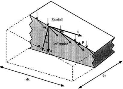
Fig. 1. Coordinate systems used for infiltration analysis on a grid element.

2. Runoff-generation module

The goal o f the runoff-generation module o f D B S I M is to obtain the spatial distribution o f the surface infiltration capacity o f the basin in order to map the evolution o f the saturated areas during a storm event. Saturation develops either near the streams, in areas o f convergence of subsurface flow, or in areas where local rainfall intensity exceeds the infiltration capacity o f the soil. A kinematic infiltration model developed by Cabral et al. (1992) which emphasizes the role o f topography in runoff generation is adapted for its use in distributed modeling by accounting for moisture transfer between elements. The result is a runoff-generation formulation which incorporates two modes o f storm runoff generation, exfiltration o f subsurface flow and infiltration-excess.

2.1. Kinematic infiltration model

The infiltration model adopted in D B S I M is based on the kinematic approximation for unsaturated flow (Beven, 1984). The kinematic model was selected for its simpli- city and computational efficiency, which favored its use f o r real-time distributed computation. The reader is referred to (Cabral et al., 1992) for a detailed description o f model conceptualization and development. Only its main results are presented here.

Basin structure and characteristics are represented on the rectangular grid defined by the digital elevation model. Each grid element consists o f a soil column of uniform slope angle a. Moisture flow is analyzed in the plane perpendicular to the soil surface along the line of maximum slope, as represented in Fig. 1. The local coordinate system follows the line of maximum slope (axis p, positive downslope) and the normal to the

(4)

282 L. Garrote, R.L. Bras / Journal of Hydrology 167 (1995) 279-306 N t n m Nf -~- Initial moisture -- Nwt n O s a t

!i! :':':':'i:i:~:~:i:i:i:~:i:~:i:i:::: Top front

iiiiiiiiiiii~!ii!iii ~ ~ S t o r m m o i s t u r e w a v e

~ etting front

Water table

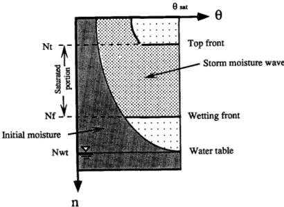
Fig. 2. Vertical moisture profile for a soil column.

soil surface (axis n, positive inward). Conditions along the line of maximum slope and in the third spatial dimension are assumed uniform. To represent a possible layering

effect, the soil is considered anisotropic, with anisotropy ratio at. The main directions

of anisotropy are parallel to the axes of the local coordinate system in every cell, so

that Kp = arK, where Kp is hydraulic conductivity in the parallel direction and K in

the normal direction. Soil properties follow the Brooks-Corey (Brooks and Corey, 1964) parameterization. The saturated hydraulic conductivity is assumed to decrease

exponentially with depth in the normal direction, from a value o f ggsa t at the surface.

The exponential decay of hydraulic conductivity is controlled by a parameter, f, which is the inverse of a length scale. This parameterization represents the effect of soil compaction and follows the experimental evidence found by Beven (1984).

Under the kinematic approximation, the capillary pressure gradient is neglected and there are no diffusive effects in the penetration of the moisture wave during a storm event. The wetting front is a sharp discontinuity that separates two areas of different moisture content. Above the front, for a constant rainfall rate R smaller than the infiltration capacity of the soil, the steady-state moisture flux in the normal direction, q, is R cos(a). Applying Darcy's law, considering that only the gravitational head gradient (cos(a)) is acting

q = K(O, n) cos(a) = Rcos(a) (1)

Hence K(O, n), the normal hydraulic conductivity at depth n for a moisture content q,

is equal to the rainfall rate R. This relationship defines the moisture profile above the

front, O(n).

The decrease of saturated hydraulic conductivity with depth may lead to the

formation of a zone of perched saturation, since moisture content O(n) must cor-

(5)

L. Garrote, R.L. Bras / Journal of Hydrology 167 (1995) 279-306 283 allow uniform moisture flux along the profile. As the wetting front proceeds downwards, it may reach the level N . where the normal moisture flux equals the saturated hydraulic conductivity and O ( N . ) = 0Sat, where 0Sa t is the moisture content at saturation. F r o m that point on, a zone of perched saturation grows, bounded by the wetting front and by a top front. Eventually, the generic moisture profile shown schematically in Fig. 2 develops. The total moisture depth stored in the soil column above the wetting front M t is divided into an unsaturated area, with moisture depth Mu, and a saturated area, with moisture depth M s.

Above the top front, unsaturated infiltration proceeds according to Eq. (1). Between both fronts, the moisture profile is saturated, and the moisture flux qsat is the harmonic mean between the saturated hydraulic conductivities at the top and the wetting fronts, affected by the factor cos(a). Below the wetting front the moisture profile, 0i(n), is that corresponding to the initial state before the beginning of the storm. On the long term, this water is kept in equilibrium by a balance of forces between gravitational and capillary head gradients. However, to be consistent with the kinematic assumption, it must be assumed that this moisture profile corresponds to a moisture flux of R i cos(a), where R i is a parameter that characterizes the initial moisture profile.

The kinematic model was developed for uniform rainfall rate R. Variable rainfall rates are handled by assuming that water gets redistributed in the soil column in order to attain uniform normal flow. This means that only a single moisture wave propa- gates downwards, regardless of the variability of rainfall intensity during the storm. An equivalent uniform rainfall rate, Re, is defined as the constant rainfall rate that would have lead to the same moisture content in the unsaturated portion of the column.

Three state variables: the wetting front depth, Nf, the top front depth, Nt, and the total moisture depth, Mt define the moisture profile. The dynamics of the soil column are governed by a system of first-order differential equations in these three state variables. Under unsaturated conditions the wetting and the top front positions coincide, and their evolution is governed by

dNf _ d N t _ (R e - Ri) cos(a) (2)

dt dt 0(Nf) - 0i(Nt)

After perched saturation has developed, the wetting and the top fronts are governed by independent evolution equations

dNf _ qsat - Ri cos(a)

dt 0Sat _ 0i(Nf) (3)

dNt _ qsat - Re cos(a) (4)

dt Osat - O(Nf)

Mass balance considerations provide the evolution equation for the third state variable, Mt

(6)

284 L. Garrote, R.L. Bras / Journal of Hydrology 167 (1995) 279-306

The first term o f Eq. (5) corresponds to the moisture increment resulting from the vertical displacement o f the wetting front. Since Mt is defined as moisture depth above the wetting front, moisture accounting should include the increment due to the incorporation o f the initial moisture profile to the reference volume. The second term accounts for surface infiltration, which is discussed in the last part of this Section. The last term corresponds to lateral subsurface inflows, Qin, and outflows, Qout, from the cell owing to interactions with contiguous cells, normalized by the horizontal area o f the element, A, and is considered next.

2.2. Moisture transfers among elements

The kinematic infiltration model is used to quantify moisture movement and storage in a soil column. D B S I M uses the kinematic infiltration model in every grid cell to account for heterogeneities in slope orientation and soil characteristics. In this distributed framework, moisture transfer among grid elements needs to be taken into account in order to represent the spatial structure o f subsurface flow at the basin scale.

Two types o f moisture transfers among elements are considered in DBSIM. First, the kinematic infiltration model applied to a single grid cell or soil column predicts deviations o f infiltrating flow from the vertical even in the case o f laterally h o m o - geneous terrain. When the model is applied to a grid cell, the horizontal component o f flow produces a net flow o f moisture across the downslope boundary, which is transmitted to the adjacent element. We refer to this as the 'intrinsic' or 'local' flow. In addition to that, the application o f the gravity-dominated model o f infiltration to every element in isolation gives different pressure and moisture distributions in every cell, which in turn lead to horizontal pressure and moisture gradients that drive lateral flow between cells. This second term is called the 'interaction' flow. Both types of moisture transfer are taken into account in a simplified manner.

The local outflow across the downslope boundary o f a grid cell, Qloc, is obtained by integrating the horizontal component of the infiltrating flow over the wetted depth along that boundary (Cabral et al., 1992). The resulting expression for the horizontal subsurface flow across a vertical cross-section is applied to evaluate topographically driven outflows from all elements in the basin. Local inflows into a certain element are given by the sum o f the local outflows from all the upstream elements draining directly into it. This mechanism accounts explicitly for the role o f topography in runoff generation because it concentrates moisture in low-lying cells, possibly leading to development of saturation in the areas of convergence of subsurface flows.

There is also a diffusive mechanism, the interaction flow, which tends to spread moisture away from the areas o f perched saturation. Interaction flows are taken into account in DBSIM through a standard finite difference procedure. It is considered that the equations describing front evolution and moisture distribution in every element are valid for the central point of the grid cell. Therefore, the infiltration model provides an estimate of water pressure distribution along the normal to the surface o f every element in its central point. Interaction flows are the moisture

(7)

L. Garrote, R.L. Bras / Journal of Hydrology 167 (1995) 279-306 285 I , . s I I A v e r a ~'~: t - N I I ! | I ... I I I ! ! ... ! ! n o |

i

_t

#

a e

n l Cell

I

n 2 Cell 2

I~ 11""

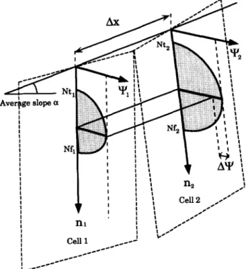
s ~ . S s S ! , o s S t s s

Fig. 3. Schematic o f pressure distributions in two contiguous cells.

transfers resulting from lateral gradients of pressure between every two adjacent cells. The evaluation of interaction flow between two adjacent cells is simplified if an average slope is considered for both cells (Fig. 3). Under that approximation, the vertical distribution of the horizontal gradient, Jx(z), along the boundary between two adjacent cells, 1 and 2, is given by

j x ( Z ) O~ll A ~ ( z ) ~I/2(Z) - f f ' l ( z ) (6)

= T x ~ ~ x - x z - x~

where kv is the pressure head, z represents vertical depth, x represents horizontal distance and 0 ~ Ox is approximated as

~,(z)

, ~ x ( z )

Neglecting the effect of slope, Ax is independent of z.

Lateral flow in the horizontal direction, qx, is given by Darcy's equation

(8)

The hydraulic gradient is given by Eq. (6). The equivalent hydraulic conductivity in

the horizontal direction,

Kxe q (z),

for the intercell distance, Ax, is approximated by the

equivalent hydraulic conductivity in the parallel direction, which in turn corresponds

1 1

to two elements of length Ax

connected in series

1 1

t x e q ( g ) ~ K p e q ( 2 ) - 2 K I s a t ( Z ) "{- 2Kfisat(Z)

(8)

Total interaction flow per unit width,

Qint,

is obtained by integrating Darcy's

equation over the saturated depth

jzsu~ jzsup

Qint = Zinf

qx(z)dz = - ~nf Kxeq(Z)Jx(z)dz

(9)

where

and

(o o

Zinf = minimum C ) ' c o s ( a ) ]

Thus, Qint

is given by

Oint --

Kxeq(Z)

if21 (z

2(z) dz (10)

inf

which, dividing in two terms and substituting the limits of integration by the appro- priate values, can be expressed as

N I N 2

..::L.. : I / I ( Z ) fcos(:) . . ~I/2(Z ) --

f

eos(~) ..LL£_

Qint =

IN' Kxeq(Z) AX dz- |~2 Kxeq(Z)-:--dz

(11)

J ~

j ~ ~ x

Substituting for the value of q l given by Cabral et al. (1992) in the first term of Eq. (11) and carrying out the integration over z

Q~nt=K°eq(N~l)[Nltexp(fN~)-N~exp(N1)f

] e x p ( f N f

1) exp(Nt 1) t- -+

NI+NIt

4 - (12) This expression can be interpreted as the moisture outflow per unit width from cell 1, Q~nt, that would be obtained if only pressure head distribution in cell 1 were considered and atmospheric pressure were assumed for cell 2.

All variables in Eq. (12) refer to values in cell 1. The second term in Eq. (11), Q~nt, would correspond to moisture inflow into cell 1 considering only pressure distribution

(9)

L. Garrote, R.L. Bras / Journal of Hydrology 167 (1995) 279-306 287 in cell 2 and atmospheric pressure in cell 1. The expression is analogous to Eq. (12), substituting 1 by 2. The net interaction outflow from cell 1, Qint, is given by the difference Qlnt - QZnt.

2.3. Runoff-generation formulation

Two modes o f runoff generation are represented in DBSIM: infiltration-excess runoff and exfiltration o f subsurface flow. Both are estimated as final output of the equations described above for the dynamics o f the soil moisture profile and lateral moisture transfer. Infiltration-excess runoff is a direct consequence o f soil infiltration capacity, designated as/max, which is in turn a function o f front position. Exfiltration is a consequence o f subsurface flows into a saturated soil column.

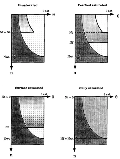
Depending on the position o f the top and the wetting fronts, the soil column can be in four distinct states, which have different runoff-generating potential. The states, represented in Fig. 4, are discussed below.

Unsaturated - - the wetting front is at some depth above the water table, but saturation has not been reached yet (Nf = Art). The soil column can only generate infiltration-excess runoff. Infiltration capacity is controlled by the saturated hydraulic conductivity at the surface

/max = K~sat c o s ( a ) (13)

Perched-saturated - - the wetting front has reached the level of saturation, but the top front is still at some depth below the surface (0 < Nt < Nf). The soil column generates infiltration-excess runoff with the same surface infiltration capacity as in the previous state (Eq. 13). Its external behavior is similar to that o f a n unsaturated cell, but, as the top front approaches the surface, the column becomes closer to saturation and the potential for generating exfiltration increases.

Surface-saturated - - the wetting front is at some depth above the water table and the top front is at the surface (N t = 0, Nf < Nwt). When the top front reaches the surface infiltration capacity is abruptly reduced to the value o f the moisture flux in the saturated part o f the soil column. Substituting for the value o f qsat given by Cabral et al. (1992).

v o f N f cos(a) (14)

/max = qsat = *'xSat e x p ( f N f ) - 1

The runoff generation properties o f the column are not a function o f the surface infiltration capacity, but o f the average infiltration capacity of all the saturated zone as a whole, which extends from the surface down to the wetting front. Since hydraulic conductivity decreases with depth, infiltration capacity is significantly lower than that o f the unsaturated case. The column may also generate exfiltration, if infiltration plus subsurface flows into the cell exceed subsurface outflows.

Fully saturated - - the wetting front has reached the water table depth, Nwt, and the top front is at the surface (Nt = 0, Nf = Nwt). The saturated zone extends down to the water table and the soil column behaves effectively as if the water table had reached

(10)

288 L. Garrote, R.L. Bras / Journal of Hydrology 167 (1995) 279-306 U n s a t u r a t e d P e r c h e d s a t u r a t e d 0 sat 0 sat 0 Nf = Nt Nt NI Nwt N ~ n n Nt---q S u r f a c e s a t u r a t e d 0 sat F u l l y s a t u r a t e d O N t = c 0 N f N w l N f = N w l n _n

Fig. 4. Four runoff-generation states for a soil column.

the surface. N o rainfall f r o m the s t o r m can infiltrate

Imax = 0 (15)

Therefore, the t e n d e n c y o f fully saturated cells to generate surface r u n o f f and subsurface exfiltration is maximized.

A c t u a l infiltration is o b t a i n e d by c o m p a r i n g the infiltration capacity o f the soil with the rainfall rate. I f the rainfall rate is greater t h a n the infiltration capacity, actual infiltration equals the infiltration capacity a n d infiltration-excess r u n o f f is generated.

(11)

L. Garrote, R.L. Bras / Journal of Hydrology 167 (1995) 279-306 289 The actual infiltration,/, is given in all cases by

I = R if R </max

/ = / m a x if R > Imax (16)

Designating the hortonian or infiltration-excess runoff by R h, it is given by

Rh = R - I (17)

Subsurface exfiltration is generated when the cell is saturated, as a consequence o f moisture balance. It is assumed in D B S I M that all moisture inflows accumulate in the area o f the soil column affected by the storm, that is, above the wetting front. There-

fore, the total moisture content has an upper limit, set by Nf0sat, which corresponds to

surface saturation. Whenever the sum of the previous moisture content in the element and the net moisture inflow exceeds the saturation volume above the wetting front, exfiltration is generated. If the cell is not saturated at the surface (unsaturated or perched-saturated states), there is a reservoir above the top front to absorb subsurface moisture inputs, and there is little chance o f exfiltration. However, if the cell reaches the surface-saturated state, the limit to the increase o f moisture content is set by the speed at which the wetting front progresses downwards, and the potential to generate exfiltration is very high. In this case, according to the moisture balance equation, exfiltration takes place whenever

I -~ Qin -- Qout/> dNf

A ~ [ÙSat -- 0i(Nf)] (18)

In that condition (surface-saturated cell satisfying Eq. 18), subsurface exfiltration, Rex is

Rex = I + Qin - Qout dNf

A dt [OSat -- Oi(Nf)] (19)

The total runoff generated by the cell is designated by Rf, and it is the sum of

infiltration excess runoff Rh, given by Eq. (17), and subsurface exfiltration Rex

given by Eq. (19)

Rf = Rex + Rh (20)

3. Surface flow routing

The formulation chosen in D B S I M to represent the distributed response o f a basin is the distributed convolution equation

QA (t) = Rf(x, y, T)h(x, y, t - T)dTdA (21)

where QA (t) is the resulting hydrograph at the outlet of a basin of area A, Rf(x, y, t) is a function describing the distribution o f runoff rate generation per unit area in the basin and h(x, y, t) is the instantaneous response function o f the element of area, dA,

(12)

located at coordinates (x, y). In a linear and time-invariant system, the instantaneous response function is constant during the event. Otherwise, the instantaneous response function may vary during the event, according to the varying transport conditions in the drainage network.

In DBSIM, the distributed instantaneous response function is assumed to be a Dirac delta function, with a delay equal to the time of travel from the location of the element to the outlet of the basin. The travel path, IT, for a typical hillslope element consists of a hillslope fraction, lh, corresponding to overland flow or diffuse flow in small gullies, and a stream fraction, Is, corresponding to concentrated channeled flow

IT = lh + ls (22)

To obtain the time of travel, velocities must be defined. Hillslope and stream velocities vary with location and must be strongly correlated with slope, and therefore a spatial distribution of velocities and hence of travel times could be obtained. However, in the absence of a sound basis to estimate the spatial distribution of velocities, mean velocity values were chosen for this work. Travel time is then defined according to the assumption of uniform velocities for both overland and stream flows throughout the basin for a given time, although travel velocities are allowed to vary as the storm progresses, accounting for the changing flow conditions in the streams. If vh (r) is the hillslope velocity and vs(r ) is the stream velocity at time r, the travel time, t~, for a typical hillslope element is given by

/h ls

t~ - vh(r---7 + vs(r~ (23)

The time-of-travel formulation allows for a simple computation of the hydrograph at the basin outlet. The instantaneous response function of the basin element located at (x, y) at time r, h~(x,y, t), is the Dirac delta function given by

h.,-(x, y, t) = 6

[ lh(x'

y) + Is(x, y)] (24)

L

vg,-) J

An incremental basin response, qar(t ) is estimated independently for every time step,

r, routing the runoff generated at every cell

qar(t) = Z R f ( x , y , r ) h ~ ( x , y , t ) A x A y (25)

(x,y)eA

where

Rf(x, y, t)

is the runoff rate generated in the element at location (x, y) at time r and xy is the area of the element. The total basin response at any time T, Q~(t), is obtained by summing the incremental responses from the beginning of the storm until current time, T

" r = T A

Q~(t) = ~ q~ (t) (26)

r = 0

(13)

L. Garrote, R.L. Bras / Journal of Hydrology 167 (1995) 279-306 291

the quick estimation o f the incremental response o f any basin once an estimate for hillslope and stream velocities is available at every time step. Currently, travel velocities are estimated in D B S I M by calibration. It is assumed that hiUslope and stream velocities are uniform t h r o u g h o u t the basin and that the ratio o f stream velocity to hillslope velocity is a constant, K v. Therefore

vh(T ) _ Vs(~-) (27)

Kv

where Kv is the ratio o f stream velocity to hillslope velocity. This simple parameterization, with values o f K v generally between 10 and 15, has been found to perform well in almost every case tested.

However, for certain basins it was found necessary to account for some non- linearities in basin response because travel times were a function o f the a m o u n t o f water present in the basin. In these cases, the mean values of hillslope and stream velocities are allowed to vary during the storm. M a n y authors (Askew, 1970; Keller- halls, 1970; Mein et al., 1974; Pilgrim, 1977) suggest that a power relation between discharge and flow velocities is valid, at least on a statistical sense. The variable selected to parameterize flow velocities in D B S I M is discharge at the basin outlet QO. Basin discharge provides a rough estimate o f the conditions in the drainage network, and has the computational advantage o f being readily available at all times. Therefore, if basin response is clearly non-linear, the following equation is applied to obtain average hillslope velocities in the basin

vh (r) = cv[Q° (T)]r (28)

Vh(T )

is the hillslope velocity at time "r, Q°(r) is the discharge at the basin outlet at time ~-, r is a calibration parameter that controls the degree of non-linearity in the basin and Cv is a calibration coefficient specific for every basin that sets the average velocities as a function o f the discharges that can be expected.

4. Model implementation

The two modules that compose DBSIM, the runoff-generation module and the surface flow routing module are integrated under a software architecture which formally maintains their independence. Model definition was conditioned to some extent by the requirement to run efficiently in a real-time flood-forecasting framework, and thus, it is expected that the lack o f detail in the representation o f certain physical processes is to some extent compensated by the possibility to use distributed modeling in this context.

As a result o f the feedback process between hydrologic modeling and software development (see G a r r o t e and Bras, this issue), the final structure o f D B S I M is particularly well suited for implementation in a real-time interactive computer environment. The state-space formulation of the runoff-generation module provides on- line evaluation of basin state evolution and allows for the implementation o f updating algorithms. In every model cell, the system o f first-order differential equations

(14)

governing infiltration is efficiently solved through an explicit finite difference scheme. Interactions among cells are recursively ordered according to the relation 'drains to'. There is no need to solve implicit numerical schemes and therefore execution time is a linear function o f the number of grid cells. The model adopted for flow routing allows the quick evaluation of storm hydrographs at any point in the basin, once the travel path and runoff have been obtained for every contributing cell. These processes of local infiltration, distributed runoff generation and surface flow routing are well differentiated and offered to the user as separate simulation tools in an interactive environment. The user can perform on-line analyses, studying the local one-dimen- sional infiltration, evaluating the runoff generation potential o f certain areas or obtaining the outflow hydrograph at any point in the basin.

5. The Sieve basin case study

Model performance was analyzed using the Sieve basin as a case study. The Sieve is one o f the tributaries o f the Arno river, which drains an area o f 8000 km 2 on the northwest o f the Italian peninsula. The confluence o f the Sieve and the Arno is located near Florence, where the area o f the Sieve catchment is approximately 840 km 2. The basin is elongated in shape, with the main river following the Southeast direction. Except in the valleys, dedicated to agriculture, the terrain is forested and moun- tainous, with an average elevation of 470 m above sea level. The elevation of the highest peak is 1657 m, and the outlet is at 50 m above sea level. The climate is Mediterranean. The rainy season lasts from October until April, with peaks in November and February.

5.1. Sensitivity analyses

The sensitivity analyses focused on variables that affect runoff generation ((1) the inverse length scale that controls the decrease o f hydraulic conductivity with depth,f, (2) the anisotropy ratio, a r and (3) the initial depth o f the water table, Nwt) and on routing parameters ((1) the ratio o f hillslope and stream velocity, Kv, (2) the coefficient c v and (3) the exponent o f the non-linear law, r). Only the main results o f the analyses are presented here. The interested reader is referred to G a r r o t e and Bras (1993) for a detailed discussion. Model sensitivity to runoff-generation parameters is presented first, followed by the study o f flow routing parameters.

The parameter values considered in the analysis o f the runoff generation are shown in Table 1. The parameters f and a r were assumed uniform throughout the basin, while the initial position o f the water table, Nwt, was allowed to vary, according the physical model o f subsurface saturated flow o f (Cabral et al., 1990). F o u r values o f the inverse scale length, f , and the anisotropy ratio, ar, were considered.

The initial state was defined by the initial wetting front depth, Nf(x, y), the water table depth, Nwt (x, y), and the initial moisture content o f the soil column above the water table, expressed in terms o f the parameter R i ( x , y ). The wetting front was assumed to be at the surface at the beginning o f the storm. Initial water table

(15)

L. Garrote, R.L. Bras / Journal of Hydrology 167 (1995) 279-306

Table 1

Parameter values for runoff generation analysis

293

Parameter Values

P a r a m e t e r f ( m m h -1) 1 × 10 -4 3 × 10 -4 5 × 10 -4 7 x 10 -n

Anisotropy ratio a r 1 10 100 500

Initial state Dry Average Wet

positions were generated using the model described by (Cabral et al., 1990), which considers Darcian water movement in the saturated zone below the water table. The model gives the water table position for which the baseflow drained from the basin is in equilibrium with a long-term recharge rate, assumed uniform throughout the basin. Three long-term recharge rates were used, corresponding to wet, average and dry states. The parameter R i is obtained at every location by requiring soil moisture to reach saturation at the depth o f the water table.

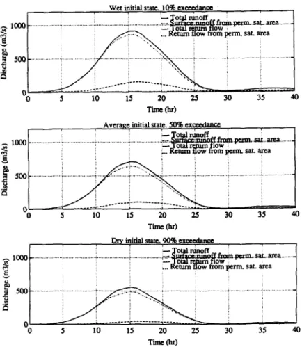
Basin responses for different parameter values are illustrated in Figs. 5-7. R u n o f f is decomposed according to its different possible origins. Two basic types o f runoff are considered: infiltration-excess runoff and subsurface exfiltration. Since basin state dynamics are also important, the plots differentiate between runoff generated in the areas o f the basin which are permanently saturated (stream areas or areas where the initial water table is at the surface) and runoff generated in the areas o f the basin which become temporarily saturated during the storm. In general, runoff generated in permanently saturated areas is not sensitive to parameter values, and is only deter- mined by the basin initial state. R u n o f f generated in the rest o f the basin can be extremely sensitive to parameter values, accounting for the visible differences at the basin scale.

The lowest part o f the runoff plots (dotted line) represents exfiltration generated in permanently saturated areas. This area is barely noticeable in most plots because the contribution o f this type of runoff to the global response is very small, in spite o f the fact that the fraction o f the basin which is saturated is important in some cases. The next layer (between the dotted and the dashed line) represents exfiltration generated in areas that have become temporarily saturated. The third layer (between the dashed and the d a s h - d o t t e d line) represents infiltration-excess runoff generated in areas permanently saturated. Since infiltration capacity here is null, these areas usually account for the most important fraction o f total runoff generation. The last fraction (between the d a s h - d o t t e d line and the solid line) represents infiltration-excess runoff generated in the rest o f the basin, and includes both the unsaturated and surface- saturated areas.

These results suggest that the representation o f hillslope processes is still incom- plete, since the fraction o f exfiltration generated in saturated areas will certainly be greater in a real basin. This p o o r result is a distortion introduced by the event-based approach adopted as modeling strategy. Given the definition o f the initial state with the wetting front at the surface, it takes some time until the storm moisture wave simulated by the model grows and reaches the permanently saturated areas, whereas in nature these areas are contributing baseflow from the beginning o f the storm. This

(16)

294 L. Garrote, R.L. Bras / Journal of Hydrology 167 (1995) 279-306 1000 IOO0 ~3 1000 50O

Wet initial state. 10% exeecdancc

i '~ ! - r o ~ runoef ': i

... ~ ... ~ ... .-.~.,. ~-tT~p~aabf~ ~om veto- sat ..area ...

! ~ ~ _ 1 Oral ~ SlOW : :

500

0

0 5 ~0 15 20 25 30 35 4o

Tinm (hr)

Average initial state. 50% ex _c~.d__ance

... ~ ... ~ , . - . ~ r ~ ~ , * m . p ~ - m . . ~ . . , ~ - ~ ...

i ~ - - _l oral ~ S l O W

~.. Return ttow n'om ~ sat. area

0

0 5 10 15 20 25 30 35 40

Time Oar)

Dry initial state. 9 0 % . . e x ~ l a n ~

. . . . . . . . .

~.. Return tlow trom penn. sat. area

. . . i . . . : .. . .

0

0 5 10 15 20 25 30 35 40

Time (hi')

Fig. 5. D e c o m p o s i t i o n o f b a s i n r e s p o n s e i n t o different m o d e s o f r u n o f f g e n e r a t i o n for i n i t i a l m o i s t u r e states w i t h 10, 50 a n d 9 0 % p r o b a b i l i t y o f exceedance. T h e results c o r r e s p o n d to p a r a m e t e r f e q u a l to 5 × 10 -4 mrrt -1 a n d a n i s o t r o p y r a t i o e q u a l t o 10.

misrepresentation cannot be corrected by simulating a longer period, prior to the beginning o f the storm, because for interstorm periods the kinematic a p p r o x i m a t i o n is not applicable at all. The effect is partly overcome by adding a baseflow term to the final hydrograph, which represents the quasi-equilibrium subsurface moisture outflow corresponding to the condition at the beginning o f the storm.

Sensitivity to the initial state is shown in Fig. 5, where basin responses to wet, average and dry initial states are shown. The model was sensitive to the position o f the water table in all cases, but it was observed that different combinations o f the other parameters can greatly enhance this sensitivity. In general, the effect o f f on the sensitivity to the position o f the water table was greater than that o f the anisotropy ratio, The definition o f the basin initial state is crucial f r o m the point of view of runoff generation, since it is the m o s t i m p o r t a n t factor governing basin response. Greater

(17)

L. Garrote, R.L. Bras / Journal of Hydrology 167 (1995) 279-306 295 P a r a m e t e r f 0.0001 ram- 1 '-- T o ~ nlnoff ' ' 1000 ... .-.,,.,~firf~emmo(f g r a m t a e n a . . s a t . a m a ... ~ ~ 1 O r a l re.,lllITI I I O W : ; : ~.. R e t u r n flow f r o m ~ sat. a r e a 500 ... .- . . . ~ . - - . . . - . . ~ . . . - . . ... ~ ... ~ ... / . .2 r~ 0 5 10 15 20 25 30 35 40 Time (hr) P a r a m e t e r f 0 . 0 0 0 3 nma-I 1000 i ~ ~ o ~ n l n o f f '~

! i.. R e t u r n tlow f r o m I mrm- sat- a r e a

0 0 5 10 15 20 25 30 35 40 Time Oar) P a r a m e t e r f 0 . 0 0 0 5 m m - I 1000 ... , ... : ... .- . , . - . . ~ f f ~ - n i n o f f I r m a 1aetna.sat, a r e a ... . ~ : - - - . . . I o t ~ t ~ l l O W : i ... ~ t u r n ttow t r o m pcrm. sat. a r e a 5 0 0 ... ~ ... , ... 0 5 10 15 20 25 30 35 40 Time (hr) P a r a m e t e r f 0 . 0 0 0 7 m m - I / i - - Toua rtlno~ !

10001- ... i ... ..-...,. ~,it;Fay, e S u i a o ~ granx .perm.. sat.. a r e a ... ... R ~ a r n n o w n o m l~rrn, sat. a r e a 0 0 5 10 15 20 25 30 35 40 Time (hr) F i g . 6. D e c o m p o s i t i o n o f b a s i n r e s p o n s e i n t o d i f f e r e n t m o d e s o f r u n o f f g e n e r a t i o n f o r p a r a m e t e r f e q u a l t o 1 x 10 - 4 , 3 × 10 - 4 , 5 x 10 -4 a n d 7 × 10 -4 m m - I . T h e r e s u l t s c o r r e s p o n d t o a n i s o t r o p y r a t i o e q u a l t o 10 a n d i n i t i a l m o i s t u r e s t a t e w i t h 5 0 % p r o b a b i l i t y o f e x c e e d a n c e .

(18)

Anisotro~ ratio I

7 -- a'o~ runoff i 7

1000 ... , ... i ... ~ ... :~= ~rfa~e~uinof~ f~mn pen~.sat, area ...

, . ~ ! :: ~ , . . , 1 0 t a , I ~ I I O W

~ i i ~.. Ketum now n'om perm. sat. area

5oo

...

i

. . . 0 0 5 I0 15 20 25 30 35 40 Time Oar) Anisotropy ratio 10 T ~ ' i i ^ ~ o o o ... ~ ... = ~ ° ~ - d ~ o ~ . ~ - , ~ . ~ , . ~ . . .

~ ! ~.. Kemrn now n'om perm. sat. area

0 5 tO 15 20 25 30 35 40 Time (hr) Anison.opy ratio 100 i - - Total nmoff ' Io0o ... i ... ~:..-. ~ Y - ~ r o m . p e r m . s a t . a r c a ... i : ~ W : : 500 ... ~ ... 0 5 10 15 20 25 30 35 40 Time (hr) . Anisotropy ratio 500,

i ~-- Total ran off ~ n s ~ ax~a

- - , ~ ... ~ ...

_~o~,,o-.S~-~:

~ , . . . ~,.. 1 ~ t l O W llrOttl l p c r m , s a t . a l e a . . .

ICIII

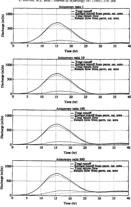
0 O 5 IO 15 20 25 30 35 40 Tune (hr)

Fig. 7. Decomposition o f basin response into different modes o f runoff generation for anisotropy ratio equal to 1, 10, 100 and 500. The results correspond to parameter f equal to 5 × 10 -4 m m -1 and initial moisture state with 50% probability o f exceedance.

(19)

Table 2

Parameter values for the sensitivity analysis o f surface flow routing

297

Parameter Values

Velocity ratio K v 5 10 15 20

Coefficient Cv (m h -1 ) 100 200 400 600

Exponent r 0.0 0.1 0.2 0.3

long-term recharge rates (wet states) lead to a greater proportion o f the basin with water table at the surface and shallower water table depths in the unsaturated areas. Basin response is directly affected by the fraction o f the basin which is initially saturated. Moreover, the tendency o f the saturated area to expand during the storm is greater for shallow water table positions, which are correlated with wet initial states. An important part o f the sensitivity of the total hydrograph to the inverse scale length, f, comes from exfiltration generated in the areas o f the basin which become saturated during the storm (Fig. 6). Also, there is a different response in infiltration- excess runoff, but it is comparatively smaller. The parameter f defines the level at which the wetting front will reach saturation for a given infiltration rate. A s f b e c o m e s greater, saturation is reached at a shallower depth, and therefore a greater number of cells become saturated. The infiltration capacity in those cells is significantly reduced and more surface runoff is generated, but the most important effect is that when a certain area becomes saturated all the subsurface flow converging into it exfiltrates. The mechanisms through which the parameter f i n c r e a s e s runoff generation are: (1) increasing the surface o f locally saturated areas; (2) enhancing the production o f exfiltration in these locally saturated areas.

As shown in Fig. 7, model sensitivity to the anisotropy ratio is smaller than sensitivity to the parameter f. In general, only the case a r -~ 500 appears to be significantly different from the rest. The cases o f a r --- 1 and ar = 10 are almost equal. The sensitivity of the total hydrograph to the anisotropy ratio is from the exfiltration generated in permanently saturated areas (dotted line in the plots). The mechanism through which the anisotropy ratio increases runoff generation is by enhancing the production o f exfiltration in permanently saturated areas. The response time o f runoff generated through this mechanism is much slower than other runoff components o f the basin. The anisotropy ratio controls lateral flow between elements, and, therefore, its main influence is through the effect o f subsurface exfiltration. As shown in Fig. 7, the portion o f exfiltration generated in the areas which become saturated during the storm is approximately constant for different anisotropy ratios. Exfiltration is mainly controlled by the parameter f , because local saturation is mostly a transient effect, and the response o f subsurface flow is so slow that there is no time to accumulate enough convergence o f subsurface flow in the temporarily saturated areas. The effect o f the anisotropy ratio is seen in the areas which are permanently saturated because, in that case, there is enough time for subsurface flow to accumulate.

Another set o f computer runs was used to test sensitivity to surface routing parameters. The model was run with a unique set o f runoff-generation parameters

(20)

2 9 8 L . G a r r o t e , R . L . B r a s I J o u r n a l o f H y d r o l o g y 1 6 7 ( 1 9 9 5 ) 2 7 9 - 3 0 6 Sensitivi~ to Kv. r = 0.1 cv = 400 mh-I 000 " I ! : i i i k-Kv=20

~15oo

. . . . . . . . . ... E ~ v ; B v ;.-Kv=II0 ! . ,~ "..! ,,-',, ! ! : . . . ? . . . " - ' : " " ' V ) . . " ' " " V . . . ! . . . , - - . K v . - - . : 5 ... " ... ~ ...

~

1000 : "" ~ ' : 500 ... ' ... ."~'-""',---~ ... ,' " ... ", ... , ... 0 5 10 15 20 25 30 35 40 45 50 Time (hi')

2000 Sensitivity to ev. Kv = I0 r = 0.I

~15oo ...

-,.-.~y....=...~..0.~ ...

i..cv=400m/h i

v

,.,

~-cv=200m/h i

~1 I D O 0 ... ." ... ~ ' - ' " : ' " ' " ' ~ ' ; . , ' : : - ' " - ' ~ - ' ~ • , m / "~ . ' . " ~ . ; . : ... ~ ... . . . ~ . - . 4 t ' ~ . m / h . . ~ . , i ~ , - - ~ v v ' o , , ~ o , , : ... , ... . J ~ i ....t., ..~ i i i i i : ! : " : ' ~ . : : : : '~U ; : i : ; " . % : ; ~ e . , l ~ ° o ° . . : : : : 500 ... i~ ... .:;i/:i.:

: ...

",..i...',.,.'..:..

i.,,... :

... ::',...,: ,, ...

~i ...

~ ...

~:'

...

o# • . . . . , ~ * . ; • . ~ . : . " ~"~ - ~ ' ' : ~"l " - ~ ' ~ : ! X m t ~ ' * " * ~ i l - - - ~ ° f ~ e i " ' a l l ~{11 I . . . ~ , . ~ [ , , T l . . . L - _ _ 5 10 15 20 25 30 35 40 45 50 Time(hr) 2000 S~sitivity to r. Kv-- 10 ¢v = 400 mh.l ! I I : ; ; : : ; . - r = 0 ~ ~ l~)O ... ". ... ";'"","'¢.::. ... ~ ... : ... ~." ... : ... :: .~ ; / ~ ~ ~ .;..r=0.2 i i ... g ... , _ . ,t...'.L...~.~,.::2...i ~ ,,: ... i ... i--.r.:.0,O ... i ... i ... 1000

500

...

:.:,.:....,.,.,:,:.,

... ~ ... :: ... i ... . ... . ' ; ' / ; , , , , i ~ i i

o

-.,~

~::i"....-.

-~ ... 50 0 10 15 20 25 30 35 40 45 Time (hr) F i g . 8. S e n s i t i v i t y o f b a s i n r e s p o n s e t o s u r f a c e f l o w r o u t i n g p a r a m e t e r s . a n d the s u r f a c e - r o u t i n g p a r a m e t e r s w e r e c h a n g e d to e x p l o r e m o d e l sensitivity. T h e p a r a m e t e r s tested w e r e the r a t i o o f s t r e a m v e l o c i t y to hillslope velocity, Kv, the coefficient ev a n d the e x p o n e n t r in the p o w e r l a w re la ting hillslope v e l o c i t y a n d d i s c h a r g e at the o u t l e t (Eq. 28). T h e n u m e r i c a l v a l u e s o f the p a r a m e t e r s are s h o w n in T a b l e 2.

(21)

L. Garrote, R.L. Bras / Journal of Hydrology 167 (1995) 279 306 299

Model sensitivities to the ratio o f velocities, Kv, to the coefficient Cv and to the exponent r are presented in Fig. 8. Sensitivity is very high in all cases and hydrograph shapes are greatly affected by the routing parameters. The effects o f Kv and Cv are very similar, because both represent uniform increments in travel velocities. In the case of Kv, the increments only correspond to stream velocities, while in the case o f Cv, the increments correspond to both stream and hillslope velocities. In both cases the effect o f decreasing the parameter value is to dampen the basin response, delaying the occurrence o f the peak and smoothing the shape o f the hydrograph. It also appears that stream velocities are dominant in configuring basin response, at least for the range o f parameter values tested here.

The effect o f the exponent r is somewhat different from that of Kv or Cv. Large values o f r narrow the shape o f the hydrograph significantly. The explanation is that increments in r represent greater increments o f travel velocities when the discharge is large, and therefore, the velocities are greater around the peak and lower at the beginning and the end of the hydrograph. This is a good criterion to identify non- linearities in basin response.

5.2. Model calibration and evaluation

Data for model calibration were taken from Cabral et al. (1990), who applied a preliminary version o f D B S I M to the Sieve basin. The D E M available for the Sieve had a resolution o f 1 m in elevation and a cell size of 400 x 400m 2. Data about physical basin parameters and several observed storms were also available. Rainfall data were available from a limited number o f recording stations at a temporal resolution o f 20 min. Streamflow data were available from a stage gauge located at Fornacina, near the confluence o f the Sieve with the Arno. The gauge did not operate continuously. It recorded water levels only during storm periods which were considered to be potentially dangerous. Hence no interstorm flow data were available. A total o f ten storm events were selected to analyze model performance. Five storms were used to calibrate the model against observed data. The resulting parameter set was then tested using the other five storms.

Most model parameters were estimated using available information on topography and soil types. The D E M provided information on slopes and drainage directions, following the methodology o f analysis proposed by T a r b o t o n et al. (1991). Soil parameters were estimated from a study by Busoni et al. (1986), which included the characterization o f 17 soil types for the Sieve basin, defining saturated hydraulic conductivity and porosity. Other B r o o k s - C o r e y parameters were estimated from published values in the literature for soils of similar conductivity and texture. Only a minimum number o f parameters were fixed by calibration: f and ar for runoff generation and Cv and Kv for surface flow routing. The goal o f calibration was to obtain reasonable parameter values that produced the best collective agreement between computed and observed streamflow in the events reserved for calibration.

During the sensitivity analyses, f and a r were found to be relatively independent. Parameter f controls the volume of infiltration-excess runoff and ar the volume of

(22)

Table 3

Parameter set which gave the best fit

Parameter Value Parameterf(mm -l) 7 x 10 -4 Anisotropy ratio a r 500 Velocity ratio K v 12.75 Velocity coefficient cv km h- l 0.408 Exponent r 0

subsurface runoff. The difference is observable, since infiltration-excess runoff is directly related to rainfall, whereas subsurface runoff m a y occur after precipitation has finished, Therefore, the tail o f the observed h y d r o g r a p h can be used to obtain an estimate o f short-term subsurface runoff adjusting the value o f a r. The other component o f runoff was then estimated by adjusting the value o f f . The process required a t h o r o u g h analysis of every storm available, to discriminate between direct and subsurface runoff. It was complicated because observations of runoff were usually discontinued when water levels returned to normal values and, therefore, only a small fraction of the tails o f the hydrographs was available.

The initial state o f the basin should be either estimated from measurements of surface moisture distribution or computed with a long-term hydro-climatological model that includes evapotranspiration. In practice, the only data available for the Sieve basin were precipitation series at the recording stations, which were insufficient to define a reasonable initial state. The solution adopted was to estimate the initial state as another u n k n o w n by calibration. Model definition o f the initial state is a function o f just one variable, the uniform recharge rate that is in long-term equilibrium with observed interstorm flows in the basin. Long-term records of streamflow in the A r n o river allow the estimation o f the distribution o f monthly averages o f interstorm flow in the Sieve. F o r every month, a value of interstorm streamflow can be assigned to a given probability o f exceedance. Flows with low probability of exceedance represent wet states and flows with high probability o f exceedance represent dry states. F o r every m o n t h three probability levels were selected: 0.1, 0.5 and 0.9, and the corresponding interstorm flows were obtained (Cabral et al., 1990).

Three initial states were thus defined for every month, and calibration was accomplished for all three states o f the corresponding m o n t h in every storm. This Table 4

Calibration: summary of results

Storm Rainfall (mm) Peak Shape Initial state Result

February 1977 33.04 Fair Fair 50-10% Fair

January 1979 46.36 Good Good 50% Good

November 1982 74.45 Fair Good 90% Good

February 1983 38.34 Good Very poor 50%? Poor

(23)

500 450 400 350 250 200 150 100 50

06

January 1985 i ! /(1~"~'~ i :~ i 10% e:~cedance !

i [.ii

k\ :~

i

. . . 50% e~cedan~:e ... ! ... ~ ~ i ~ ,< ... i i ... i ... ~ - 5 1'0 15 20 25 30 35 40 45 50 Time (hr) 301

Fig. 9. Observed and simulated hydrographs for the storm of January 1985. Simulated results correspond to initial moisture states with 10, 50 and 90% probability of exceedance.

approach weakens the soundness o f the calibration process, since much o f the variability in basin response can be explained through different initial conditions, but no other independent means of estimating the initial state were available.

The scheme followed in the calibration o f the time o f travel was much simpler because the hypothesis o f uniform hillslope and stream velocities throughout the basin reduces the complexity o f the problem. The drainage network was defined independently o f the calibration. The network proposed by Cabral et al. (1990), based on studies of Carlfi et al. (1987), was adopted. The network is generated from the D E M following drainage directions and using a threshold contributing area o f eight elements, which corresponds to 1.28 km 2. The resulting network had 1084 stream elements out o f a total o f 5252 for the whole basin; this high density o f stream elements is due to the coarse spatial resolution of the D E M available.

Travel velocities are given by Eqs. (27) and (28). The parameters to estimate are the coefficient Cv and the exponent r, and the ratio o f stream velocity to hillslope velocity, K v. The exponent r was initially set to 0, since there was no special reason to expect

Table 5

Verification: summary of results

Storm Rainfall (ram) Peak Shape Initial state Result

December 1968 31.77 Poor Fair 90-50% Fair

January 1969 41.56 Good Good 90% Good

December 1975 52.67 Poor Fair 90% Poor

December 1976 26.61 Fair Fair < 10% Fair

(24)

302 600 500 400 ~ 300 ~5 200 100

L. Garrote, R . L . Bras / Journal o f H y d r o l o g y 167 (1995) 2 7 9 - 3 0 6

December 1968 T / ' - t ... i ... ! ... 7 "t/"ik ... i ... i .... ~0%~Xc~dan,~e ... i i ! 1 ; ~ \ \ i i . . . 50% eXcedanee J i i ] ~ ' , ' ~ ;" ~;/,~ i i ... 90% exc:ddan~e

...

~ ...

~ , ; ; : ~ i i i

... i ...

"~.:;2

"~:¢"~' ... ! ...

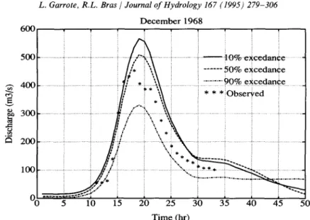
5 10 15 20 25 30 35 40 45 50 Time (hr)

Fig. 10. Observed and simulated hydrographs for the storm of December 1968. Simulated results correspond to initial moisture states with 10, 50 and 90% probability of exceedance.

non-linearity. The estimation o f Cv and Kv was based on the comparison o f the general features o f the hydrograph, notably the time at which the main peak occurs.

A trial-and-error process was followed during calibration. Once satisfactory values for the routing parameters were obtained, different combinations o f f and ar were tried until acceptable results were obtained. The objective o f the calibration was to obtain a rough estimate o f the approximate values o f the parameters, since a mathematical parameter optimization could not be carried out because o f a lack of enough streamflow information.

The selection o f the best parameter set was made based on a comparison o f the observed data with the simulations corresponding to the three initial conditions. The objective was to reproduce qualitative features of the observed flow, such as peak discharge, time to peak and baseflow recession. Since the initial state was not known, there was one degree o f freedom in the results. The evaluation of the results was subjective, and the assumption was made that the storms available for calibration should be comprised between the two limiting initial conditions, 10% and 90% probability o f exceedance, respectively. The parameter set which gave the best fit is listed in Table 3. It is remarkable that the best fit is obtained with an anisotropy ratio o f 500.

A subjective evaluation o f the calibration results is presented in Table 4. Two qualitative variables are included in the analysis:

peak

and

shape. Peak

includes the ability to reproduce the values and especially the timing o f the observed peak discharge. Timing is considered more important than absolute value, because the simulations cover a wide range of possible values, owing to the uncertainty o f the initial

state.

Shape

is an overall evaluation of how the simulated hydrographs reproduce the

(25)

L . G a r r o t e , R . L . B r a s / J o u r n a l o f H y d r o l o g y 1 6 7 ( 1 9 9 5 ) 2 7 9 - 3 0 6 303 N o v e m b e r 1991 1 2 0 0 ... ~ ... ~ ... [ ! ... i t O % . - e x c e d a n c e ... 1 0 0 0 ~ i LF" ' --- 50°, exc~dance i *"~'~t...." ... ~'-" 9 0 % e x c e d a n c e 8 0 0 , ] i ~ * , * Observe~

..

,.t=

~ 600

~ ...

::i

... ~i ... . I. ...

~

~ *

...

i::

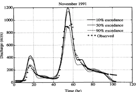
... 4 0 0 . . . ~ ... i ... ",... ... ~ ... ~ ... 2 0 0 . . . . i . " . . , . . . 2 0 4 0 6 0 8 0 1 0 0 1 2 0 T i m e ( h r )

Fig. 11. O b s e r v e d a n d s i m u l a t e d h y d r o g r a p h s for the s t o r m o f N o v e m b e r 1991. S i m u l a t e d results corre- s p o n d to initial m o i s t u r e states w i t h 10, 50 a n d 9 0 % probability o f exceedance.

o f the initial state that leads to the best fit between observed and simulated hydrographs.

Peak discharge and time to p e a k are reasonably well reproduced. However, the overall shape o f the simulated h y d r o g r a p h s is not as well preserved. Total runoff volumes obtained in the simulations a p p e a r to be larger than observed ones, but no conclusive assessment can be m a d e owing to the lack o f continuous streamflow recording. As an illustration o f the type o f results obtained, model results for the storm o f J a n u a r y 1985 are shown in Fig. 9.

The predictive capability o f the calibrated model was tested in the verification step using other five storms. The model was run with the o p t i m u m p a r a m e t e r set obtained in the calibration, and results were c o m p a r e d with observed discharge data.

A subjective evaluation o f the results, considering the same criteria used in the calibration step, is presented in Table 5. Although differences between observed and simulated h y d r o g r a p h s are apparent, model p e r f o r m a n c e with the verification set is no worse than with the calibration set, which suggests that the calibration process was successful in the sense o f estimating the best p a r a m e t e r set for the basin. I f these other five storms were included in a new calibration process, the values of the p a r a m e t e r s p r o b a b l y would not change very much.

C o m p a r e d with the calibration set, a greater dispersion with respect to the initial state is observed in the verification set. While the D e c e m b e r 1976 storm appears to correspond to a very wet initial state, the storms of J a n u a r y 1969 and D e c e m b e r 1975 suggest a very dry initial condition. In general, model p e r f o r m a n c e is acceptable in all storms except in N o v e m b e r 1987. An example o f the results obtained is presented in Fig. 10 for the storm o f D e c e m b e r 1968.

(26)

304 L. Garrote, R.L. Bras / Journal o f Hydrology 167 (1995) 279 306

storm in the Sieve basin. The storm took place in November 1991, and the quality of the data was significantly better than that of the previously available storms. Rainfall information was still obtained from a rain gauge network, but network density was considerably greater. A total of 30 rain gauges were available, and six o f them were located inside the Sieve basin. Total rainfall depth in the basin was 111 ram. Stream- flow data were also o f greater quality, since continuous recording o f streamflow was available.

The model was run for this recent storm, and the results are shown in Fig. 11. The results are very encouraging. The model reproduces the shape of the hydrograph with reasonable accuracy, and model performance is better than in the other cases of the verification set and even the calibration set. The simulation suggests a relatively dry initial condition, which is consistent with the time of the year (beginning of the rainy season). The timing of the rising and the falling limbs of the hydrograph is acceptable, and the adjustments o f the interstorm periods are excellent, specially if we consider that poststorm baseflow recession is generated through physically based mechanisms using the same parameters as other model processes, and not through conceptual recession equations with specific parameters to fit baseflow recession.

Although such good model performance with a good data set could very well be just a serendipitous coincidence, it strongly suggests that model performance can be considerably improved with better data. In particular, distributed rainfall information obtained from radar maps is crucial to evaluate the response of the different areas of the basin to irregularly distributed rainfall.

6. Concluding remarks

The Distributed Basin Simulator, a rainfall-runoff model for real-time flood forecasting in midsize and large basins is presented. D B S I M accepts distributed rainfall input and uses intensively the topographical information encoded in the DEM, as well as other types of georeferenced information. It accounts for the effects of slope, anisotropy and soil heterogeneity on subsurface flow and runoff production through an analytical formulation of local infiltration processes. Basin-scale processes of surface and subsurface water transport are also represented through discretized schemes on a rectangular grid. The model emphasizes computational efficiency for real-time use, although the main features of topography-based runoff generation and transport processes are believed to be well represented.

D B S I M was tested on a 840 km 2 watershed in the Arno basin (Italy), under the average conditions that can be expected in a practical application, using a short record o f ten events. Model performance was first analyzed through extensive sensitivity analyses followed by a calibration and verification exercise. The sensitivity analyses gave an appreciation o f the role of model parameters in the generation of basin response. The parameter f w a s found to control mostly the volume of infiltration-excess runoff, whereas the anisotropy ratio ar was found to control the volume o f subsurface exfiltration. However, actual calibration values obtained for these parameters cast some doubts over the possibility of estimating them exclusively from