C H A R A C T E R I Z I N G CHAOS IN A T Y P E OF F R A C T I O N A L D U F F I N G ' S EQUATION
S. JIMÉNEZ AND P E D R O J. ZUFIRIA
ABSTRACT. We characterize the chaos in a fractional Duffing's equation com-puting the Lyapunov exponents and the dimension of t h e strange attractor in the effective phase space of the system. We develop a specific analytical method to estimate all Lyapunov exponents and check the results with t h e fiduciary orbit technique and a time series estimation method.
1. Introduction. In a previous work [1] a fractional Duffing's equation was studied in the presence of both harmonic and nonharmonic external perturbations, the later arising from Geometrical Resonances. An attractor, similar to the strange attractor of the classical (i.e., non fractional) Duffing's equation was identified.
In this present work, we characterize the chaotic behaviour of solutions of the fractional equation computing the Lyapunov characteristic exponents and the Lya-punov dimension of the attractor for different values of the fractional parameter a. To achieve this, we build a local equation for perturbed solutions. This apporach is new, to the best of our knowledge.
Given the paradigmatic role of Duffing's equation in the Theory of Dynamical Systems, the fractional counterpart we consider may reflect the relevant features of many other models. Hence a motivation for this study. Besides, chaos in fractional Duffing's equations has been studied but many questions remain open.
In section 2 we give a brief description of the classical Duffing's equation, we present a fractional counterpart and the numerical method we have used to sim-ulate it. In section 3, we review the basic features of the Lyapunov characteristic exponents and present a method for to the specific case of the fractional equation that allows us to compute all the exponents. We also consider the Lyapunov di-mension of the system. In Section 4 we present the numerical results obtained from our simulations, with the new method, the fiduciary orbit technique and the time series estimation method. Finally, Section 5 summarizes the conclusions.
2. Dufflng's equations.
2.1. The classical Dufflng's equation. Duffing's equation has served as a par-adigm for many studies on chaotic systems described by a time-forced, dissipative, second order nonlinear differential equation [2].
Different terms can be considered but what we may call the basic equation corre-sponds to a model for a long and slender vibrating beam set between two permanent magnets, subjected to an external sinusoidal force. The equation is [2]
x + 7¿ — x + x =/ocos(wt), (1)
where the dots represent derivation with respect to time. The parameters in the equation are: the dissipation coefficient 7 > 0, the intensity /o of the external force and its angular frequency u>. Varying the values of these parameters a wide range of different behaviours can be observed in the system [3]. Chaos and a strange attractor appear in the numerical simulations for a relatively wide sets of values. A typical choice of the parameters for which chaos is observed corresponds to 7 = 0.25,
w = l,f0 = 0.3
2.2. Fractional Dufflng's equations. Several fractional variantions of the clas-sical Duffing's equation have been considered by different authors, depending on which fractional derivative is considered and what integer order derivative it re-places [4, 5]. In our case, we replace the first order derivative by a fractional one:
x + 7_D"x — x + x3 = /ocos(wt), (2)
with a G (0,1). We consider the Caputo fractional derivative with expression:
^
x
M = T^)£itt)£-»
dT
>
(3)
where n is the integer part of a + 1 (supposed a > 0), t > to a nd T(-) is Gauss'
gamma function. In our case, we will fix to = 0 and consider a £ (0,1) (and, thus,
n = 1), and use the following simplified notation [1]:
1 /"' X'(T)
D?x(t) = — r / , ^ ; dT, (4)
* V ' r ( l - a ) i o {t-r)« K '
where the prime in x' represents derivation with respect to the variable. In the limit
a —> 1, the fractional derivative tends to the first order derivative and the fractional
equation has Duffing's equation as its limit.
2.3. Numerical method. We have performed numerical simulations of Equation (2) approximating the fractional derivative with Diethelm's method [9] and using a Strauss-Vázquez approach (see the ODE part of [10]) for the other terms, as was done in [1]. The evolution equation for the discrete variable xn is:
• ^ n + l ¿Xn \ Xn—\ ^f
b? haT{2 •
n-l
xn—k x0 ) k = l
o 2 2 S
xnJrl ~r %n—l xnJrl ~r xnJrlx,n—l T ^ n + l ^n— 1 ~r xn—l
2 4 cos(wín +i)+cos(wín_i)
— Jo 2 ' ^ ' where h is the time-mesh step, tn = nh and the coefficients Ckn correspond to [9]:
COn = 1 ,
Ckn = (k + 1)1-" -2k1-a + (k-l)1-a, 0<k<n, (6) cnn = (1 - a)n~a - nl-a + (n - l )1" " .
At startup, for n = 1, we have a three level discrete equation and the initial values are used to provide both starting values XQ and x\. We have that XQ = x(0), while to compute x\ we approximate by a Taylor expansion of a sufficient order, namely:
h2 h3
Xl=X0 + hVQ + —XQ + —XQ. ( 7 )
Supposing that the initial values satisfy the equation at t = 0, we have:
x0 = x0 - x% + /o , x'o = v0 - 3XQWO • (8)
Assuming x(t) to be regular such that x exists, implies that all the fractional derivatives involved are zero at t = 0 (see [6]), hence these two last equalities. Once the values of xn are known, the corresponding values of the velocity vn can
be computed using a suitable representation of the first order derivative. More information about this method can be found in [1].
3. Lyapunov Characteristic exponents.
3.1. General properties. Lyapunov Characteristic Exponents (LCE) are a stan-dard tool to characterize the chaoticity of solutions of a differentiable dynamical system (see, for instance, [11, 2, 15] and references therein).
They are defined for a differentiable map / , such that xn+i = f(xn), through
Os-eledec's multiplicative ergodic theorem (see, for instance, [11, 16]) as the logarithms of the eigenvalues of the limit:
lim ( J " * J " )1 / 2 n, Jn = j(p-\x0))---j(f{x0))J{x0), (9) n^rco
where J(-) is the Jacobian matrix of the map, XQ is the solution of the dynamical system at the initial time and * denotes the adjoint matrix.
The fact that the LCE are defined as limits at an infinite time supposes a prob-lem which is tackled in practice computing the logarithms of the eigenvalues of
(Jn* Jn) ' n, up to a large time-step n, and considering that they represent well
the asymptotic behaviour as the time goes to infinity.
Although the LCE's are also defined for flows, in practice it is seldom possible to apply the definition and approximation by discrete maps are used. For a dynamical system given by
i=F{t,x), (10)
usually a discrete map that gives the evolution of x after a prescribed (small) time step, At, is associated: x(t + At) = f(x(t)). This map is then used to compute the LCEs.
The LCE's measure the expansion or contraction of the phase space locally around a given orbit. Due to this, as a feature, for a dynamical system of dimension
N, we have [11]
N 1 f T
T,
X3=£%of
V-
F(
f^)
dt(H)
or, using the Jacobian J of the flow and, also, in the case of a discrete map:
N 1 fT
E
Ao = lim — / trace J(x) dt, (12) J T^OO T nFor instance, in the case of Duffing's equation (N = 2), we have trace J = 7, independently of (x,v) and, thus,
N
$ > ¿ = 7 - (13)
J = I
3.2. LCE for the fractional equation. Let be (x,v) some solution of our equa-tion (2) corresponding to the initial data x(0) = XQ, V(0) = VQ, and let be (y,u) some other "close" solution. The difference between both solutions is governed by the system:
x — y = v — u,
where, in our case,
v-ü=-U'{x)-U'{y)-"iD?{x-y), ^
U{x) = -l-x2 + \ x \ (15)
The linearized equations for 5 = x — y, r¡ = v — u, around a reference solution (x, v) are
i1=-U"{x)5-1D?5. <=^ \ ñ=-U"(x)S-j-r^ r [ -^—dr .
1 V ' ' * ' ' K ' T ( l - a ) J0 ( Í - T ) « (16) The study of LCE for dynamical systems is grounded on the computation of a matrix equation from which to estimate the Lyapunov spectrum. Here we may obtain such matrix equation, under the assumptions mentioned below, via the replacement of the second equation in (16) by a local approximation.
When computing a solution that is slightly perturbed from a reference solution, we may suppose that they are both identical, up to machine precision, for a given range of times, say t G [0,ti], and that they only differ after that specific time
t\. It is known [6] that Caputo derivative at time t is zero whenever the first
the integral in (16) to provide a small contribution. It has been numerically checked that whenever close to each other solutions are obtained, their fractional derivatives remain also close. We may, thus, approximate the equation for i) by:
i]= -U"{x)5-1- 1
T](T)
• dr.
T{l-a)Jtl ( i - r ) ° - - ( 1 7 )
Let us consider now t = t\ + At, with At a small step (for instance, the time-step of the numerical method we use to compute the values of both the reference solution and the perturbed one). After substitution in (17) we have at time t:
1 ftl+At V(r)
1)= -U"{x)5-1
r(i
(ii + At - T) (IT . (18)If At is small enough, we may approximate rj in the integral by its Taylor expansion around t = t\ + At:
(r-tf
V(r)=v(t) + (r-t)ri(t) +
-m
(19)and we have:
i] = -U"(x)6-i
= -U"(x)S-1
-1
r ( i - a ) At1""
íi + Aí
V + 1 (1
7?(t) + (r - t! - At)?i(t)
( Í ! + A Í - T ) «
a ) A t2-a
dr
-r] + 0(At 3-a\ (20)
r ( 2 - a ) ' ' r ( 3 - a )
The truncation order determines the maximal embedding dimension where to char-acterize the system. In order to use the same framework as in the classical case, we have limited the present study to second order.
We may, thus, approximate (17) by:
1 • 7 " (1
)At 2-c T ( 3 - a ) This is a linear system given by
/ °
= V,
= -U"(x)6-~f At1 (21)
r(2
V"
U"(x)
1 A t1" "
- 7 "
1- 7( 1
r(3
-At2 - a (22)
cr(2 - a)
We may now apply the usual technique and compute both LCEs using J\ as the effective Jacobian of the matrix equation for the difference between the perturbed orbit and the fiduciary one. Since our model corresponds to computing the LCE for a linear equation with jacobian J-¡_, the following conservation law should hold:
7 ( 2 - a ) A t1-a
Ai + A2 = trace J\ = (23)
T ( 3 - a ) - 7 ( 1 - a ) A i2- ° '
3.3. Lyapunov Dimension. The Lyapunov Dimension for a given solution that tends towards the stange attractor is defined as [14]
k
D
L=k +
T^Y,X
j, (24)
|A, fc+H J = I
with k such that Ai + • • • + A& > 0, and Ai + • • • + A^ + Afc+i < 0. It is related to
and the box counting procedure in the case of dissipative systems [15]. In our case, whenever the maximum LCE is positive, this dimension corresponds to
D
L= l + -£-
(25)
lA2|
if we consider the phase space to be two-dimensional. Alternatively, time can be included as an additional variable. Since this does not bring any new information, we will consider (25) as stated.
3.4. Other approaches. In order to check the results of the linear approximation given by the matrix equation (22), we have used the fiduciary orbit technique, that approximates the maximum LCE computing the sepparation increase of a slightly perturbed solution to a fiduciary one [12]. Also, we have used a time series approach [13] to perform a correlation dimension estimation as an alternative measure of the dimension of the attractor. The advantage of both these techniques is that no a
priori knowledge of the system is necessary, such as its dimension or its nature,
and, hence, they provide an independent information.
4. Numerical results. In the previous work [1] it was reported for the fractional equation how, with the same parameter values as for the chaotic regime in the classical Dufiing's equation, almost periodic solutions were identified as well as chaotic solutions. For instance, for 7 = 0.25, u> = I, fo = 0.3, we obtain with the initial data XQ = 0.8, VQ = 0., a solution to the fractional equation with stroboscopic cuts at multiples of the external force period 2n/ui corresponding to a strange attractor. We have represented it for the case a = 0.5 in Figure 1. It is similar in shape to the classical attractor, but is more spreaded.
1
0.8
0.6
0.4
* 0.2
0
-0.2
-0.4
-0.6
-1.5 -1 -0.5 0 0.5 1 1.5
F I G U R E 1. Strange attractor for the fractional Dufiing's equation, a = 0.5
For many different initial data, regular solutions instead of chaotic ones are found. In fact, for values of a smaller than 0.4, it becomes difficult to find initial data that do not correspond to regular solutions. These solutions are almost periodic in time as was described in [1]. This is not, in general, the case for the classical Dufiing's equation.
*n=0.8, vn=0.
We have computed the approximations to the LCEs for both kind of solutions. The results for the chaotioc solution are presented in Figure 2: we plot versus t the estimation of both LCE, Ai and A2 computed by the QR method, and of Amax
computed by the fiduciary orbit method. We see the agreement of both results, even though the estimates for Ai obtained are a little greater than those given by Amax, and that the approximation to the maximal LCE is clearly positive, as an indication of the chaoticity.
The computations have been performed with different values of the time-step h. All the results obtained are consistent with the graphics we present.
0.4
0.3
0.2
0.1
<< 0
-0.1
-0.2
-0.3
-0.4
0 1000 2000 3000 4000 5000 6000 7000
t
F I G U R E 2. Estimates of the LCE for the fractional Duffing's
equa-tion, chaotic solution.
In Figure 3 we present the same as in Figure 2 but for one of the regular solutions. We see, again, a good agreement between both methods for the maximal LCE. Now both LCE are negative.
Throughout our computations we have checked the conservation law (23). To illustrate this, we represent in Figure 4, sepparately, both Ai + A2 and trace J\ for the two solutions, the regular one and the chaotic one, of the previous Figures. We see that the agreement is satisfactory.
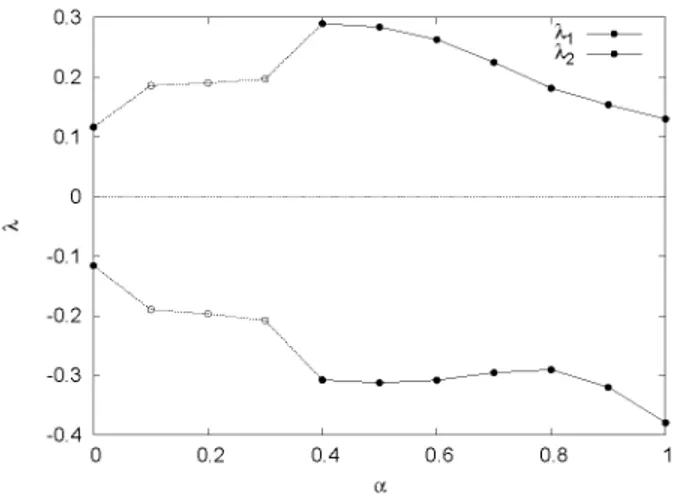
We have computed both A12 for different values of a. We represent this in Figure 5. The values of the limiting cases a = 0 and a = 1 have been obtained with the corresponding non-fractal equations: Duffing's for a = 1 and a forced Hamiltonian equation that has chaotic solutions for small amplitudes for a = 0.
From the LCE approximations, we have computed the Lyapunov dimension _D¿ given by (25). We present in Figure 6 the results for different values of a, and for the two limiting cases. For values 0 < a < 0.4, after some transient, most of the solutions seem to show regular behavior. The simulation times should be extended to clarify whether chaos always ends up showing up. To indicate this, data for 0 < a < 0.4 are represented via a dashed line in both Figures 5 and 6.
We have compared the Lyapunov dimension with the correlation dimension pro-vided by a time series method and found a good agreement. In Figure 7 we present the correlation dimension as the slope in a log-log plot for the case a = 0.5. Assum-ing 1 to be the maximal embeddAssum-ing dimension, the correlation dimension obtained
0.1
0.05
0.05
--0.1
0 1000 2000 3000 4000 5000 6000 7000
F I G U R E 3. Estimates of the LCE for the fractional Dumng's equa-tion, regular solution
^
0.002
0 0018 0.0016
0.0014
0.0012
0.001
0.0008
0.0006
0.0004
0.0002
0
«r
-*
-A=7i/300, regular solution A=7i/300, chaotic solution ÍF7I/900
-*
1000 2000 3000 4000 5000 6000
F I G U R E 4. Accuracy of the conservation law: relative error of the sum of the LCEs with respect to the trace J\ for different time-steps
reaches this maximal value, indicating that the dimension of the attractor must be greater than 1. Assuming 2 to be the maximal embedding dimension, a correlation dimension of 1.976 is obtained, consistent with the computed Lyapunov dimension. 5. Conclusions. The approximation to the LCE we present is consistent with what is computed by other methods. We conclude that this method is a practical tool for the fractional Dumng's equation we have considered. This approach can also be extended to other fractional equations since our linear, local approximation seems to be qualitatively correct and quantitatively reasonable. We have also found a good agreement among all the estimations for the effective attractor dimension within the assumed framework.
0.3 ,
0.2
-0.1 '-'"
0
--0.1 ,r
0.2
0.3
0.4
-0.2 0.4 0.6
FIGURE 5. Estimates of the LCE versus a
2
<H1.9
1.8
1.7
1.6
1.5
1.4
1.3
-0.2 0.4 0.6
F I G U R E 6. _D¿ computed with the estimates of the LCEs, versus a Since depending on a and the dimensional framework, system may show quite different behaviours, we intend to carry out further studies.
R E F E R E N C E S
[1] S. Jiménez, J. A. González and L. Vázquez, Fractional Duffing's equation and geometrical resonance, International Journal of Bifurcation and Chaos, 2 3 (2013), 1350089-1—1350089-13.
[2] J. Guckenheimer and Ph. Holmes, Nonlinear oscillations, dynamical systems, and bifurcations of vector fields, Springer-Verlag, New York, 1986.
[3] S. Jeyakumari, V. Chinnathambi, S. Rajasekar and M.A.F. Sanjuán, Vibrational resonance in an asymmetric Duffing oscillator, International Journal of Bifurcation and Chaos 21 (2011), 275-286.
[4] X. Gao and J. Yu, Chaos in t h e fractional order periodically forced complex Duffing's oscil-lators, Chaos, Solitons and Fractals 24 (2005), 1097-1104.
F I G U R E 7. Estimation of the correlation dimension assuming max-imal embedding dimensions 1 and 2, for a = 0.5
[6] A.A. Kilbas, H.M. Srivastava and J.J. Trujillo, Theory and Applications of Fractional Differ-ential Equations, North-Holland Mathematics Studies 204, Elsevier, The Netherlands, 2006. [7] R. Gorenflo, F. Mainardi, Fractional Calculus: Integral and Differential Equations of
Frac-tional Order, in Fractals and FracFrac-tional Calculus in Continuum, Mechanics (eds. A. Carpinteri and F. Mainardi), Springer Verlag,(1997), 223-276.
[8] V. Volterra, Theory of junctionals and of integral and integro-differential equations Dover Publications, Inc., USA, 1959.
[9] K. Diethelm, N.J. Ford, A.D. Freed and Yu. Luchko, Algorithms for the fractional calculus: A selection of numerical methods, Computer Methods in Applied Mechanics and Engineering
194 (2005), 743-773.
[10] S. Jiménez, P. Pascual, C. Aguirre and L. Vázquez, A Panoramic View of Some Perturbed Nonlinear Wave Equations, International Journal of Bifurcation and Chaos 14 (2004), 1—40. [11] J.-P. Eckmann and D. Ruelle, Ergodic theory of chaos and strange attractors, Reviews of
Modern Physics 57 (3) (1985), 617-656.
[12] M. Casartelli, E. Diana, L. Galgani and A. Scott, Numerical computations on a stochastic parameter related to the Kolmogorov entropy, Physical Review 1 3 A (5) (1976), 1921—1925. [13] R. Brown, P. Bryant and H.D.I. Abarbanel, Computing the Lyapunov spectrum of a
dynam-ical sustem from an observed time series, Physdynam-ical Review 5 7 A (6) (1991), 2787—2806. [14] P. Frederickson, J.L. Kaplan, E.D. Yorke And J.A. Yorke, The Liapunov Dimension of Strange
Attractors, Journal of Differential Equations 49 (1983), 185—207.
[15] H.D.I. Abarbanel, Analysis of observed Chaotic data, Springer-Verlag, New York, 1996. [16] P. Walters A dynamical proof of the multiplicative ergodic theorem Transactions of the