QUALITY OF LIFE AND POVERTY: MEASURING AND COMPARABILITY
MERCEDES MOLPECERES-ABELLA
Dept. de Econom´ıa Aplicada, Universidad de Valladolid, Avda. Valle de Esgueva 6, 47011 Valladolid, Spain
JOS ´E LUIS GARC´IA-LAPRESTA
PRESAD Research Group, BORDA Research Unit, IMUVA, Dept. de Econom´ıa Aplicada, Universidad de Valladolid, Avda. Valle de Esgueva 6, 47011 Valladolid, Spain
In this paper, we analyze the correspondence among the rankings of the Spanish regions according to different measures of monetary poverty and quality of life, in 2012. To do that, the Spearman’s rank correlation coefficient is used. Different aggregation methods are applied to calculate the selected measures of poverty and quality of life. The monetary poverty measures aggregate the income gaps, while the quality of life measures aggregate a set of social indicators dealing with ten different domains. In both cases, among other traditional aggregation procedures, the exponential mean is used because its properties are especially adequate in these contexts.
Keywords: Quality of life; poverty; aggregation functions; exponential means; dual de-composition.
1. Introduction
For decades, poverty has been a central issue in Economy (see Rowntree31, Orshansky29, Atkinson1,2and Chakravarty and Muliere9, among others). Its defini-tion and measurement can be based on the use of objective or subjective indicators and adopt an absolute or a relative approach (see Sen34,35).
According to Eurostat15, the relative approach based on income has been cho-sen in Europe to show that poverty is related to social exclusion in accordance with many previous studies (see Townsend42 and Hagenaars22). So that, it can be assumed that being poor depends on the living conditions, not on how individuals feel about them (see Ringen30), and that poverty in advanced countries can be rea-sonably defined in relative terms as persons not having resources enough to achieve a minimum acceptable way of life in the country they belong to (see Townsend41). Then, population can be divided into the poor and the non-poor, according to an income poverty line or threshold set at a fixed percentage of the median income (see Fuchs17). This paper focuses on this kind of poverty measures and sets the poverty line at the 60% of the median equivalent disposable income, as in many national,
regional and international studies (see Buhmann et al8, OECD26 and Atkinson2, among others). It allows us to identify the poor but the problem of aggregation still persists: how to combine income distribution and the poverty line in order to construct a poverty measure. Considering their properties (see Subramanian40), two different families of poverty measures have been selected to provide a compar-ative analysis for the Spanish regions (at NUTS2 level) in 2012: the Foster-Greer-Thorbecke class16and the one introduced by Garc´ıa-Laprestaet al.18. According to the Spearman’s coefficient, it has been established that regional poverty rankings do not change significantly when the importance given to inequality among the poor is altered.
No doubt, poverty is important to rank societies from the best to the worst. But it has been suggested that a more varied set of characteristics should be taken into account to generate this kind of rankings. Literature on quality of life might be the answer to that requirement (see Stiglitzet al.39). Although it is a more elusive, con-troversial and complex than poverty, quality of life is usually defined by identifying its main domains (i.e., health status, social support, income, poverty, environmental quality, personal security, etc.). Among all the methodologies proposed to measure quality of life, the most widespread consists in aggregating a set of social indicators that capture its principal domains (see Nardo et al.25 and OECD27,28). Following these premises, we propose several tentative quality of life measures: one ordinal composite index (see Slottje36, Slottje et al.37 and Dasgupta and Weale11) as well as several cardinal composite indices based all of them in the same set of social indicators (see Booysen7). All of them are used to rank Spanish regions from the highest to the lowest quality of life. These new regional rankings do not change sub-stantially according to Spearman’s coefficient regardless of the composite quality of life measure used.
In fact, both types of regional rankings result to be surprisingly similar, al-though the information used to obtain them is obviously much more restrictive in the case of the monetary poverty rankings. None of these concordances have been obtained adopting a subjective approach to elaborate quality of life rankings based on satisfaction with life (see Diener13).
2. Preliminaries
Vectors in [0,∞)m are denoted as x= (x
1, . . . , xm); in particular, 0= (0, . . . ,0) and 1= (1, . . . ,1). Given x,y ∈[0,∞)m, by x≥y we mean xi ≥yi for every i∈ {1, . . . , m}, and by x>y we mean x≥y and x6=y.
Given x∈[0,∞)m, the increasing and decreasing reorderings of the coordinates of x are denoted as x(1) ≤ · · · ≤ x(m) and x[1] ≥ · · · ≥ x[m], respectively. Con-sequently, x(1) = min{x1, . . . , xm} = x[m], x(m) = max{x1, . . . , xm} = x[1] and x[k]=x(m−k+1) for every k∈ {1, . . . , m}.
Given a setI, with #I we denote the cardinality ofI.
Aweak order(orcomplete preorder) is a complete and transitive binary relation. With and ∼ we denote the asymmetric and the symmetric parts of the weak order, respectively.
2.1. Aggregation functions
We now introduce standard properties of real functions on [0,1]m and aggregation functions. For more details, see Beliakov et al.6, Grabischet al.21 and Beliakov et
al.5.
Definition 1. Let A: [0,1]m−→R be a function. (1) Aisidempotent if for every x∈[0,1]: A(x·1) =x.
(2) Aissymmetricif for every permutation σ on {1, . . . , m} and every x∈[0,1]m: A(xσ(1), . . . , xσ(m)) =A(x).
(3) Aismonotonic if for all x,y∈[0,1]m: x≥y ⇒ A(x)≥A(y). (4) Aisstrictly monotonicif for all x,y∈[0,1]m: x>y ⇒ A(x)> A(y). (5) Aiscompensative if for every x∈[0,1]m: x
(1) ≤A(x)≤x(m). (6) Aisself-dual if for every x∈[0,1]m: A(1−x) = 1−A(x). (7) Aisanti-self-dual if for every x∈[0,1]m: A(1−x) =A(x).
(8) A isinvariant for translations if for every x∈[0,1]m and every t ∈
R such that x+t·1∈[0,1]m: A(x+t·1) =A(x).
(9) Aisstable for translations if for every x∈[0,1]m and every t∈
R such that
x+t·1∈[0,1]m: A(x+t·1) =A(x) +t. Definition 2. Let A(m)
m∈N be a sequence of functions, withA
(m): [0,1]m−→ R and A(1)(x) =x for every x∈[0,1].
(1) A(m)
m∈N isinvariant for replications if for all x∈[0,1]
m and any number of replications t∈N of x:
A(tm)( t
z }| {
x, . . . ,x) =A(m)(x). (2) A(m)
m∈N isdecomposableif, for any given subset of variables, every variable
subset without altering the overall aggregated value of the full set of variables; for instance if
A(m)(x1, . . . , xk, xk+1, . . . , xm) =
=A(m)A(k)(x1, . . . , xk), . . . , A(k)(x1, . . . , xk), xk+1, . . . , xm, for all x∈[0,1]m and k∈ {1, . . . , m}.
Definition 3. A function A: [0,1]m−→[0,1] is called anaggregation function if it is monotonic and satisfies the boundary conditions A(0) = 0 and A(1) = 1.
The dual decomposition of an aggregation function A: [0,1]m−→[0,1] in the
core
b
A(x) = A(x)−A(1−x) + 1 2
and theremainder
e
A(x) =A(x)−A(bx) =
A(x) +A(1−x)−1 2
can be found in Garc´ıa-Lapresta and Marques Pereira19.
Given α 6= 0, the exponential mean Aα : [0,1]m −→ [0,1] is the aggregation function defined as
Aα(x) = 1 αln
eαx1+· · ·+eαxm
m .
Every exponential mean is continuous, idempotent, symmetric, strictly mono-tonic, compensative, stable for translations and decomposable.
On the use of the dual decomposition of aggregation functions to welfare eco-nomics, see Garc´ıa-Lapresta et al.18, Aristondoet al.3,4 and Garc´ıa-Lapresta and Marques Pereira20.
We now describe the dual decomposition of exponential means (see Garc´ıa-Lapresta and Marques Pereira19 for more details).
Given α6= 0, thecore of Aα is the aggregation function Aαb : [0,1]m−→[0,1]
defined as
b
Aα(x) = 1 2αln
eαx1+· · ·+eαxm
e−αx1+· · ·+e−αxm .
The core of every exponential mean is continuous, idempotent, symmetric, strictly monotonic, compensative, stable for translations, self-dual and invariant for replications. Consequently, it can be considered as a position measure.
Given α6= 0, theremainder of Aα is the mapping Aαe : [0,1]m −→R defined
as
e
Aα(x) = 1 2αln
(eαx1+· · ·+eαxm)(e−αx1+· · ·+e−αxm)
m2 .
0 if and only if x1 =· · · =xn. Consequently, it can be considered as an absolute dispersion measure in the sense of Mart´ınez-Paneroet al.24whenever α >0, since
e
Aα(x)≥0 for everyx∈ [0,1]m; if α <0, then
e
Aα(x)≤0 for everyx∈[0,1]m and Aαe is an absolute dispersion measure excepting the sign, that now is negative.
We now show the parameter limits of the exponential means and their remain-ders (see Prop. 35 of Garc´ıa-Lapresta and Marques Pereira19):
(1) lim
α→∞Aα(x) =x(n). (2) lim
α→−∞Aα(x) =x(1). (3) lim
α→∞Aα(e x) =
x(n)−x(1)
2 .
(4) lim
α→−∞Aα(e x) =−
x(n)−x(1) 2
It is important noticing that Aα(x) =Abα(x) +Aeα(x), for every x∈[0,1]m.
2.2. Spearman’s rank correlation coefficient
Let S be a weak order on the set of objects O = {o1, . . . , om}. The position of object oi∈O inS is defined as
pS(oi) =m−#{oj ∈X |oioj} −1
2#{oj ∈(O\ {oi})|oj ∼oi}. (1) These positions can be also obtained as the average of the corresponding ones after a linearization process (see Smith38and Cook and Seiford10).
Example 1. Consider the weak orderS on O={o1, . . . , o8} depicted as follows S
o2o5 o1 o3o7o8
o4o6
Then,
pS(o2) =pS(o5) = 8−6− 1
21 = 1.5 = 1 + 2
2 , pS(o1) = 8−5−1
20 = 3,
pS(o3) =pS(o7) =pS(o8) = 8−2−1
22 = 5 =
4 + 5 + 6
3 ,
pS(o4) =pS(o6) = 8−0− 1
21 = 7.5 = 7 + 8
Definition 4. Given two weak orders S and T on O ={o1, . . . , om}, the Spear-man’s rank correlation coefficient betweenS andT is defined as
ρ(S, T) = 1 m · m X i=1
pS(oi)− 1
m m X i=1 pS(oi) !
· pT(oi)− 1
m m
X
i=1 pT(oi)
!! v u u t 1 m · m X i=1
pS(oi)− 1 m
m
X
i=1 pS(oi)
!2 · 1 m· m X i=1
pT(oi)− 1 m·
m
X
i=1 pT(oi)
!2
.
Taking into account that m
X
i=1
pS(oi) = m
X
i=1
pT(oi) =
(m+ 1)·m 2 and after some simplifications, we obtain
ρ(S, T) = m
X
i=1
pS(oi)− m+ 1
2
·
pT(oi)− m+ 1
2 v u u t m X i=1
pS(oi)−m+ 1
2 2 · m X i=1
pT(oi)− m+ 1
2
2
.
This coefficient lies between −1 and 1. When two weak orders are identical (perfect positive correlation) it follows that ρ(S, T) = 1. If one is the reverse of the other (perfect negative correlation), then ρ(S, T) =−1. The higher is the absolute value of the coefficient, the stronger is the intensity of rank correlation.
The statistic for testing the null hypothesis of independence H0, ρ(S, T) = 0, is:
tm−2=
ρ(S, T)√m−2
p
1−(ρ(S, T))2, (2)
according to a Student’st-distribution with m−2 degrees of freedom.
3. Poverty
We consider a population consisting of n individuals, with n≥2. Anincome distri-bution is represented by a vector x= (x1, . . . , xn)∈[0,∞)n, where xi represents the income of individual i∈ {1, . . . , n}.
The set of poor individuals in the population is denoted by Q(x, z) ={i∈ {1, . . . , n} |xi< z}, and q(x, z) denotes the number of the poor, q(x, z) = #Q(x, z).
Definition 5. For all x∈[0,∞)n and z∈(0,∞), thenormalized gap of individual
iis defined as
gi= max
z−x
i z ,0
.
Notice that gi ∈ [0,1], gi = 0 ⇔ xi ≥ z, and gi = 1 ⇔ xi = 0. In addition, the normalized gaps are invariant under proportional income changes, i.e., the function G: [0,∞)n×(0,∞)−→[0,1]n defined as G(x, z) = (g
1, . . . , gn) is homogeneous of degree 0: G(λ·x1, . . . , λ·xn, λ·z) =G(x1, . . . , xn, z) for every λ >0.
We now introduce a special notation for the incomes and normalized gaps of the poor individuals in the population: q = q(x, z), xp = (x(1), . . . , x(q)) with x(1) ≤ · · · ≤ x(q) < z, and gp = (g[1], . . . , g[q]) with g[1] ≥ · · · ≥ g[q] > 0, and g[i]= (z−x(i))/z for i= 1, . . . , q.
3.1. Poverty measures
There exist in the literature a number of poverty measures. According to Sen33and Jenkins and Lambert23, every poverty measure should be expressed as a function of three poverty indicators, the so called three I’s: incidence, intensity and inequality of poverty.
For our analysis we have selected two families of parameterized poverty measures that meet at least two out of the three Sen’s requirements: the poverty measures proposed by Fosteret al.16 and Garc´ıa-Laprestaet al.18.
First we introduce the Foster-Greer-Thorbecke (FGT) poverty measures. Definition 6. Given α ∈ [0,∞), the FGTα poverty measure is the function
FGTα: [0,∞)n×(0,∞)−→[0,1] defined as
FGTα(x, z) = 1 n
q
X
i=1 g[i]α.
Notice that FGT0 is theheadcount ratio, H(x, z) = q
n,
The next poverty measures were introduced and analyzed by Garc´ıa-Lapresta
et al.18.
Definition 7. Given α∈(0,∞), thepoverty measure associated with Aα is the function Pα: [0,∞)n×(0,∞)−→[0,1] defined as
Pα(x, z) =
H(x, z)·Aα(gp) = q n·
1 αln
eαg[1]+· · ·+eαg[q]
q , if q6= 0,
0, if q= 0.
The poverty measure Pα satisfies some interesting properties (see Garc´ıa-Laprestaet al.18 ):
(1) Poverty Focus: poverty should not depend on the non-poor incomes.
(2) Normalization: if all the individuals are non-poor, then the society deprivation level is equal to 0.
(3) Poverty Symmetry: no other characteristic apart from the income deprivation matters in defining a poverty index.
(4) Replication Invariance: if the population is replicated, then poverty should not change; this allows comparing populations of different sizes.
(5) Poverty Monotonicity: poverty should increase if a poor income decreases. (6) Transfer Sensitivity: greater weight should be placed on the poorer incomes and
poverty should decrease if inequality among the poor decreases.
(7) Diminishing Transfer Sensitivity: the poverty reduction effect of a “poor to poorer” progressive transfer should decrease as the income of the poorer person increases.
The axiomatic approach, together with the presence of the three I’s of poverty, set a list of properties that any reasonable poverty measure should satisfy. A number of different axioms exist in literature and the consistency among them have been widely analyzed (see, for instance, Donaldson and Weymark14). Table 1 summarizes the properties satisfied for each of the considered poverty measures.
Table 1. Properties of the poverty measures.
Property FGT0 FGT1 FGTα (α >1) Pα
Poverty Focus Yes Yes Yes Yes
Normalization Yes Yes Yes Yes
Poverty Symmetry Yes Yes Yes Yes
Replication Invariance Yes Yes Yes Yes
Poverty Monotonicity No Yes Yes Yes
Transfer Sensitivity No No Yes Yes
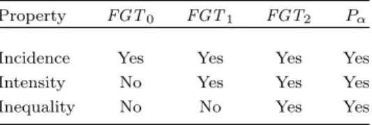
Table 2 shows whether the three I’s (incidence, intensity and inequality) are captured by each of the considered poverty measures.
Table 2. The three I’s of the poverty measures. Property FGT0 FGT1 FGT2 Pα
Incidence Yes Yes Yes Yes
Intensity No Yes Yes Yes
Inequality No No Yes Yes
According to Garc´ıa-Laprestaet al.18, for every α >0, the poverty measure Pα associated with Aα can be decomposed in the following way:
Pα(x, z) =
(
H(x, z)·Aα(b gp) +Aα(e gp)
, if q6= 0,
0, if q= 0.
Thus, the poverty measure Pα is clearly expressed through the three I’s (inci-dence, intensity and inequality), by means of H, Aαb and Aα, respectively.e H is
the classical measure for estimating the poverty incidence. As mentioned above, Aαb
is continuous, idempotent, symmetric, strictly monotonic, compensative, stable for translations, self-dual and invariant for replications, therefore it can be considered as a good measure of the poverty intensity when it is applied to the normalized gaps of poor individuals. In turn, Aαe is continuous, symmetric, anti-self-dual, invariant
for translations, invariant for replications, and it is 0 if and only if all the inputs are the same. Consequently, Aαe is a good measure of the poverty inequality when
it is applied to the normalized gaps of poor individuals.
3.2. Regional poverty comparisons in Spain
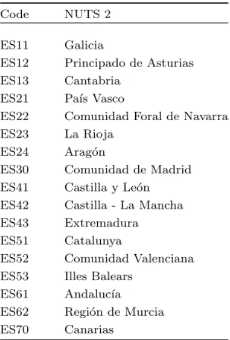
As a case of study, we propose testing at ordinal level the consistency of the poverty analysis for the Spanish regions at NUT2 level, following the Eurostat’s nomencla-ture (see Figure 1 and Table 3), using simultaneously the two families of parame-terized poverty measures presented in Subsection 3.1: FGTα (α≥1) and Pα.
Spanish regions have been ranked, the region with the lowest level of poverty achieving the first position, and so on, according to six poverty measures corre-sponding to different values of α for the two families of poverty measures defined above. All of them present different levels of sensibility towards people living with lower levels of income. In particular, the higher the parameter α, the bigger the level of sensitivity of each measure towards the poorest population, and the higher the poverty measure value obtained.
Table 3. Spanish regions and their codes.
Code NUTS 2
ES11 Galicia
ES12 Principado de Asturias ES13 Cantabria
ES21 Pa´ıs Vasco
ES22 Comunidad Foral de Navarra ES23 La Rioja
ES24 Arag´on
ES30 Comunidad de Madrid ES41 Castilla y Le´on ES42 Castilla - La Mancha ES43 Extremadura ES51 Catalunya
ES52 Comunidad Valenciana ES53 Illes Balears
ES61 Andaluc´ıa ES62 Regi´on de Murcia ES70 Canarias
households enjoy economies of scale in consumption, an equivalence scale is needed to approximate an equivalent concept of income able to reflect differences in well-being derived from differences in household sizes. As there is not an accepted method for determining equivalence scales, here we use the parametric family of equivalence scales proposed by Buhmannet al.8.
Definition 8. Let Xh be the disposable income for householdhand nh its size (the number of persons living together in the household pooling incomes and sharing consumption options). The equivalent income, xi, is defined as
xi= Xh
nθ h ,
where θ∈[0,1] represents the economies of scale derived from household consump-tion.
The larger the parameter θ, the smaller the economies of scale assumed. In our calculations we have applied moderate economies of scale, θ= 0.5. Equiv-alent income for every household is assigned to all its members, assuming that equivalent disposable income is pooled and shared equally among all of them.
Equivalent disposable incomes are then used to calculate all the poverty mea-sures selected to rank Spanish regions and test the consistency between them using the Spearman’s rank correlation coefficient.
ES11
ES12 ES13 ES21
ES22
ES23
ES24
ES30 ES41
ES42 ES43
ES51
ES52
ES53
ES61
ES62
ES70
Fig. 1. Spain map regions.
different poverty measures.
Table 4. Spearman’s rank correlation coefficients.
FGT1 FGT2 FGT10 P1 P2 P10
FGT1 1 0.9461 0.5907 0.9975 0.9951 0.9387
FGT2 1 0.6985 0.9412 0.9387 0.8529
FGT10 1 0.5833 0.6005 0.6618
P1 1 0.9975 0.9412
P2 1 0.9485
P10 1
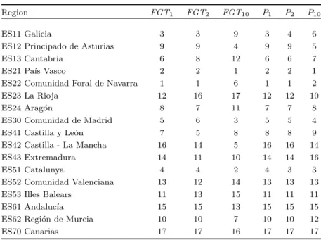
the top of the ranking. And for other four regions (ES13, ES30, ES42 and ES53) the differences among their ranks do not exceed two positions (see Table 5). Therefore, results suggest a high level of consistency among relative regional positions based on income poverty, regardless of the measure or the level of sensibility towards poor people with lower income levels.
Table 5. Ranks of poverty in the Spanish regions.
Region FGT1 FGT2 FGT10 P1 P2 P10
ES11 Galicia 3 3 9 3 4 6
ES12 Principado de Asturias 9 9 4 9 9 5
ES13 Cantabria 6 8 12 6 6 7
ES21 Pa´ıs Vasco 2 2 1 2 2 1
ES22 Comunidad Foral de Navarra 1 1 6 1 1 2
ES23 La Rioja 12 16 17 12 12 10
ES24 Arag´on 8 7 11 7 7 8
ES30 Comunidad de Madrid 5 6 3 5 5 4
ES41 Castilla y Le´on 7 5 8 8 8 9
ES42 Castilla - La Mancha 16 14 5 16 16 14
ES43 Extremadura 14 11 10 14 14 16
ES51 Catalunya 4 4 2 4 3 3
ES52 Comunidad Valenciana 13 12 14 13 13 13
ES53 Illes Balears 11 13 15 11 11 11
ES61 Andaluc´ıa 15 15 13 15 15 15
ES62 Regi´on de Murcia 10 10 7 10 10 12
ES70 Canarias 17 17 16 17 17 17
It is generally accepted that societies with low levels of poverty, however it was defined and measured, are preferred to those with high levels of poverty contributing to raising quality of life. Considering the consistency shown by the regional rankings based on different measures of poverty, the question arises about what would be the effect on rankings if other social indicators related to quality of life were included. The approach of the synthetic measures of the quality of life can help us to answer that question, since its sole purpose is to summarize the most relevant information provided by a set of the quality of life indicators.
4. Quality of life
It may not be possible to define an objective synthetic measure of quality of life, but societies have to evaluate alternative social states. Organized objective data is needed to closely monitor social well-being. Research has resulted in different quality of life composite indices (for pros and cons of composite issues, see Nardo
et al.25).
According to the principle of parsimony, the proposed Composite Measures of Quality of life (CMQ) are based on a selection of few relevant social indicators dealing with different issues (like health or inequality) that affect individuals and society as a whole. Controversial indicators have been excluded. Indicators inter-acting with each other, yet not measuring the same phenomena, have been included (for example, income and inequality).
Many different methodologies can be used to evaluate social quality of life and results depend on the methodology finally applied. None of them have been gen-erally accepted for any society at any time, but experts agree that a high degree of transparency is required about methodological choices. Among all of them, com-posite indices provide clear advantages over competing methodologies: they have a multidimensional nature but, at the same time, synthesize numerous indicators into a single number which facilitates comparisons among territories and over time. Composite indexing entails the aggregation of different social indicators. It involves three steps: data selection (dimensions and indicators), standardization and aggre-gation.
4.1. Data selection
Measuring quality of life requires selecting social indicators that suitably capture any of its dimensions. They must be chosen on the basis of their analytical sound-ness, measurability, region coverage and relevance to the quality of life. There is no single definitive set of dimensions or indicators and proxy measures have to be used when desired data is unavailable. Each indicator, viewed individually, will show a social problem improving or worsening. All of them interrelate and contribute to the overall quality of life. We consider seven dimensions and ten social indicators (see Table 6 for more details).
• Dimension 1: Material living conditions.
machine a colour TV; a telephone.
• Dimension 2: Inequality.
3. Income inequality: Gini coefficient for equivalized disposable income.
• Dimension 3: Health status.
4. Life expectancy: Life expectancy at birth.
5. Population without disabilities: Share of individuals aged over 15 with-out problems of mobility, for self-care or daily activities or suffering pain, discomfort, anxiety or depression.
• Dimension 4: Work and human capital. 6. Unemployment: Unemployment rate.
7. Human capital: Share of tertiary education employed in the science and technology sector.
• Dimension 5: Social capital.
8. Help from others: Share of individuals who have the possibility to ask for help (any kind of help: moral, material or financial) from any relatives, friends or neighbours who don’t live in his or her household.
• Dimension 6: Personal security.
9. Crime: Share of individuals who have crime, violence or vandalism prob-lems related to the place where they live.
• Dimension 7: Environmental quality.
10. Environmental problems: Share of individuals who have pollution, grime or other environmental problems related to the place where they live such as: smoke, dust, unpleasant smells or polluted water.
Table 6. Selected social indicators.
Indicator Source Year Quality of life
1. Average equivalized disposable income EU-SILC 2012 increases 2. Severe material deprivation EU-SILC 2012 decreases
3. Income inequality Own∗ 2012 decreases
4. Life expectancy Eurostat 2012 increases
5.Population without disabilities INE 2012 increases
6. Unemployment INE 2012 decreases
7. Human capital INE 2012 increases
8. Help from others EU-SILC 2012 increases
9. Crime EU-SILC 2012 decreases
10. Environmental problems EU-SILC 2012 decreases
4.2. Standardization
The essential reason why it may be necessary to scale variables is that raw data can have significantly different ranges. So that, without scaling, composite indices will be implicitly weighted towards variables with large ranges. This will imply that small but meaningful changes in an indicator will insignificantly affect the composite index.
The Linear Scaling Technique (LST) is likely to be the most common procedure to standardize the ranges of variables, including the Human Development Index43. It deals with the directionality issue and provides a consistent way to aggregate variables when some of them contribute to increase and others to decrease quality of life32. LST assumes that the empirically observed values of a variable represent its feasible range and that movement in it can be best expressed as a fraction of that feasible range. To do this, an estimate is made for the highest (max) and lowest (min) values for all regions.
Whenever there is a variable increase which corresponds to an increase in the overall quality of life, then it is scaled according to the following formula
Ikj = X j
k−minXk maxXk−minXk
,
whereIkj is the index score corresponding to thek-th social indicator for the region j and maxXk and minXk are the maximum and minimum values of the k-th social indicator for all the considered regions, respectively.
In contrast, whenever a variable increase corresponds to a decrease in the overall quality of life, then it is scaled according to the following formula
Ikj = maxXk−X j k maxXk−minXk
.
In both cases, the ranges of values are in the unit interval, where the lowest level of quality of life is scored at 0 and the highest is set at 1.
4.3. Aggregation
Probably, aggregation is the most controversial issue in the construction of compos-ite indices. A standard approach to aggregation is the addition of all components to form the composite index. We have selected two different aggregation methods. An ordinal one, based on the Borda rule. And, accordingly with one of the poverty measures used above, Pα, the exponential means. Both of them are advantageous because of its methodological transparency. In addition, exponential means can be decomposed into two components: the core; and the remainder, which measures to what extent disparities among different social indicators contribute to reduce quality of life. It shows preference for regions with similar values for all the social indicators considered.
on the relative importance of each of the facets of the quality of life considered. Sec-ond, ask experts or policy makers for their relative valuations. Both assignments of weights suffer from disadvantages linked to the fact that people’s preferences can be non-transitive, specially when the number of variables grows. The third alternative is the use of statistical techniques such as Principal Component Analysis, which usually result on small weights for social indicators with little variation despite of their intrinsic importance for quality of life.
For now, equal weights are given to all the standardized variables, as in Slottje36 and in the Human Development Index43.
The ordinal Composite Measure of Quality of life for the region j, CMQor, corresponds just to the sum of a region positions in the rankings according to all the standardized social indicators considered:
CMQor= 10
X
k=1 pjk,
wherepjk is the position of regionj in the weak order dealing with indexk. In turn, the family of cardinal Composite Measures of Quality of life CMQjα, with α <0, correspond to the exponential mean of the scoresIkj for each regionj:
CMQjα=AαI1j, . . . , I10j = 1 αln
10
X
k=1 eαIkj
10 .
We have considered α <0 for ensuring that CMQjα will be smaller in regions with marked deficiencies in any of the considered aspects of quality of life, even though they were well placed with respect to the rest of them. That is, in regions with similar values for all the indicesIkj.
All the synthetic indices proposed above have been calculated for the Spanish regions in 2012. Estimations have been used to rank regions according to quality of life. According to each synthetic index, first position has been assigned to the region with the highest value, that is, the highest quality of life, and so on. This results in so many regional rankings as quality of life indices obtained. The issue about their consistency arises again, and Spearman’s rank correlation coefficient is used to analyse this matter (see Table 7).
Table 7. Spearman’s rank correlation coefficients. Quality of life indices.
CMQor CMQ−1 CMQ−2 CMQ−10
CMQor 1 0.9975 0.9902 0.9044
CMQ−1 1 0.9951 0.9191
CMQ−2 1 0.9338
Our results suggest that all the rankings, based on ordinal aggregation as well as cardinal aggregation, even for very high absolute values ofα, tend to assign very similar positions to the Spanish regions in 2012 according to quality of life. That is, the Spearman’s coefficients are significant (at the 0.05 level of significance) and very close to 1.
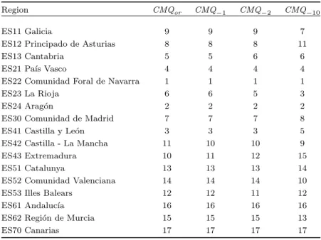
In fact, five regions out of the seventeen considered maintain the same position whatever the measure of quality of life used (ES21, ES22, ES24, ES61 and ES70), three of them are at the bottom of the ranking. Four regions lose only one position (ES13, ES30, ES51 and ES53), two of them being at the end of the ranking. And other five regions (ES11, ES22, ES41, ES42 and ES62) present differences between ranks that do not exceed two positions (see Table 8). Again, as in the poverty case, the consistency among different measures is very high for the Spanish regions in 2012.
Table 8. Quality of life in the Spanish regions.
Region CMQor CMQ−1 CMQ−2 CMQ−10
ES11 Galicia 9 9 9 7
ES12 Principado de Asturias 8 8 8 11
ES13 Cantabria 5 5 6 6
ES21 Pa´ıs Vasco 4 4 4 4
ES22 Comunidad Foral de Navarra 1 1 1 1
ES23 La Rioja 6 6 5 3
ES24 Arag´on 2 2 2 2
ES30 Comunidad de Madrid 7 7 7 8
ES41 Castilla y Le´on 3 3 3 5
ES42 Castilla - La Mancha 11 10 10 9
ES43 Extremadura 10 11 12 15
ES51 Catalunya 13 13 13 14
ES52 Comunidad Valenciana 14 14 14 10
ES53 Illes Balears 12 12 11 12
ES61 Andaluc´ıa 16 16 16 16
ES62 Regi´on de Murcia 15 15 15 13
ES70 Canarias 17 17 17 17
indices, that is: its top position in the ranking is associated to high values in all the indicators selected. ES70 (Canarias) is in the opposite situation, at the bottom of the ranking and with a low discount because of the remainder component, that is: its bad position in the ranking is due to low quality of life indices in all the considered aspects.
Regions with the highest discounts linked to differences among indices are ES43 (Extremadura), at the bottom of the ranking, and ES30 (Comunidad de Madrid) and ES12 (Principado de Asturias), around the middle of it. For example, Comu-nidad de Madrid presents the highest levels for life expectancy, share of population without disabilities and tertiary educated employed in science and technology sec-tor, but at the same time very high shares of individuals who declare suffering from crime and environmental problems. Data suggests that in Spanish regions in 2012 high or low differences among indices can be found at any position in the quality of life ranking.
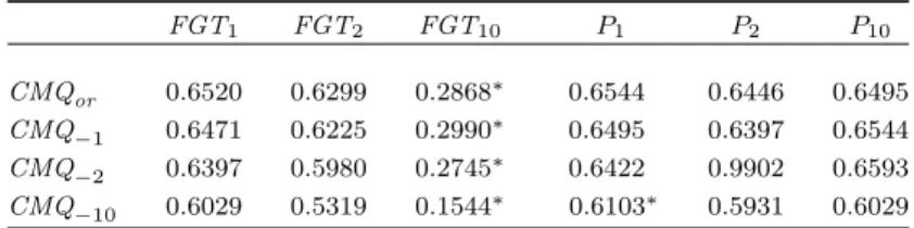
4.4. Comparing poverty and quality of life rankings for the Spanish regions
The main objective is now analyze if poverty measures used in Section 3, so con-sistent among them, are good proxies for the composite measures of quality of life proposed in this section, which are also consistent among them. In other words, if regional rankings on poverty and those on quality of life are equivalent or not for Spanish regions in 2012. Spearman’s rank correlation coefficients are still high (see Table 9), although smaller that those obtained above (see Table 4 and Table 7). No doubt it is due to the different nature of the concepts compared, being quality of life much broader than income poverty. In any case, it is noteworthy that most of the Spearman coefficients, close to 0.6, and statistically significant. Except those corresponding to FGT10, probably because of the higher importance given to big poverty income gaps. Concluding, data suggests that the Spanish regions where income poverty is low (on the top of the poverty ranking) tend to be regions where quality of life is high (top positions on the quality of life ranking). This makes poverty measures acceptable proxies for the Spanish regions’ quality of life in 2012 .
4.5. Subjective quality of life
Table 9. Spearman’s rank correlation coefficients. Poverty measures and quality of life indices.
FGT1 FGT2 FGT10 P1 P2 P10
CMQor 0.6520 0.6299 0.2868∗ 0.6544 0.6446 0.6495
CMQ−1 0.6471 0.6225 0.2990∗ 0.6495 0.6397 0.6544
CMQ−2 0.6397 0.5980 0.2745∗ 0.6422 0.9902 0.6593
CMQ−10 0.6029 0.5319 0.1544∗ 0.6103∗ 0.5931 0.6029
∗Not significant at 0.05 level of significance
of Diener12): “Although subjective well-being is not sufficient for the good life, it appears to be increasingly necessary for it”.
Here we compare regional rankings on quality of life, based on the synthetic measurements proposed above, with the regional ranking on life satisfaction. The results suggest that there is no correlation among them. None of the Spearman’s rank correlation coefficients are significant. Even more, it is not correlated with poverty rankings presented in Section 3. This result is consistent with studies on adaptation of individuals to new situations by changing their expectations or rela-tive subjecrela-tive well-being which must be evaluated in a social context being affected for the relative situation of the reference group.
5. Concluding remarks
The study of Spanish households’ equivalent disposable income in 2012 shows that regions do not substantially alter their position in the ranking when the poverty measurement’s sensitivity towards disparities among poor incomes changes. The high values of the Spearman’s ranks correlation coefficient confirm this point.
A similar conclusion is obtained by using different composite measures of quality of life. Spanish regions tend to maintain similar positions in the ranking, regardless the ordinal or cardinal approaches to quality of life measurement. The same is true when the possibility of trade-offs between progress and setbacks in different social indicators is modified. Regions on the top and regions on the bottom of the quality of life ranking tend to be the same.
Comparing both kinds of rankings, we get a curious conclusion. Monetary poverty rankings, based on a one-dimensional view (equivalent disposable income), are surprisingly similar to rankings on quality of life, based on a multi-dimensional view (combinations of ten social indicators). It configures poverty measurements as an acceptable proxy for composite measures on quality of life, a possibility that would be desirable to explore in other contexts.
ranks correlation coefficients is significant, in accordance with the literature on this field.
Further research may incorporate other social indicators’ weighting schemes or modifications on the selected set of social indicators in order to confirm or refuse the obtained conclusions.
Acknowledgments
J.L Garc´ıa-Lapresta acknowledges the funding support of the SpanishMinisterio de Econom´ıa y Competitividad(project ECO2012-32178) andConsejer´ıa de Educaci´on de la Junta de Castilla y Le´on (project VA066U13).
References
1. A.B. Atkinson, On the measurement of poverty,Econometrica 55(1987) 749–764. 2. A.B. Atkinson,Poverty in Europe(Blackwell, Oxford, 1998).
3. O. Aristondo, J.L. Garc´ıa-Lapresta, C. Lasso de la Vega, R.A. Marques Pereira, The Gini index, the dual decomposition of aggregation functions, and the consistent mea-surement of inequality, International Journal of Intelligent Systems 27(2012) 132– 152.
4. O. Aristondo, J.L. Garc´ıa-Lapresta, C. Lasso de la Vega and R.A. Marques Pereira, Classical inequality indices, welfare and illfare functions, and the dual decomposition, Fuzzy Sets and Systems 228(2013) 114–136.
5. G. Beliakov, H. Bustince Sola and T. Calvo S´anchez,A Practical Guide to Averaging Functions(Springer, Heidelberg, 2016).
6. G. Beliakov, A. Pradera and T. Calvo,Aggregation Functions: A Guide for Practi-tioners (Springer, Heidelberg, 2007).
7. F. Booysen, An overview and evaluation of composite indices of development,Social Indicators Research59(2002) 115–151.
8. B. Buhmann, L. Rainwater, G. Schmaus and T.M. Smeeding, Equivalence scales, well-being, inequality, and poverty: sensitivity estimates across ten countries using the Luxembourg Income Study (LIS) database,The Review of Income and Wealth34
(1988) 115–142.
9. S.R. Chakravarty and P. Muliere, Welfare indicators: A review and new perspectives. 2. Measurement of poverty, Metron - International Journal of Statistics 62 (2004) 247–281.
10. W.D. Cook and L.M. Seiford, On the Borda-Kendall consensus method for priority ranking problems,Management Science 28(1982) 621–637.
11. P. Dasgupta and M. Weale, On measuring quality of life, World Development 20
(1992) 119–131.
12. E. Diener, Subjective well-being: the science of happiness and a proposal for a national index,American Psychologist 55(2000) 34–43.
13. E. Diener, Guidelines for national indicators of subjective well-being and ill-being, Journal of Happiness Studies 7(2006) 397–404.
14. D. Donaldson and J.A. Weymark, Propeties of fixed-population poverty indices, In-ternational Economic Review 27(1986) 667–688.
16. J. Foster, J. Greer and E. Thorbecke, A class of decomposable poverty measures, Econometrica52(1984) 761–766.
17. V.R. Fuchs, Redefining poverty and redistributing income, The Public Interest 8
(1967) 88–95.
18. J.L. Garc´ıa-Lapresta, C. Lasso de la Vega, R.A. Marques Pereira and A.M. Urrutia, A class of poverty measures induced by the dual decomposition of aggregation functions, International Journal of Uncertainty, Fuzziness and Knowledge-Based Systems 18
(2010) 493–511.
19. J.L. Garc´ıa-Lapresta and R.A. Marques Pereira, The self-dual core and the anti-self-dual remainder of an aggregation operator,Fuzzy Sets and Systems159(2008) 47–62. 20. J.L. Garc´ıa-Lapresta and R.A. Marques Pereira, The dual decomposition of aggrega-tion funcaggrega-tions and its applicaaggrega-tion in welfare economics,Fuzzy Sets and Systems 281
(2015) 188–197.
21. M. Grabisch, J.L. Marichal, R. Mesiar and E. Pap,Aggregation Functions(Cambridge University Press, Cambridge, 2009).
22. A. Hagenaars,The Perception of Poverty (North-Holland, Amsterdam, 1986). 23. S. Jenkins and P. Lambert, Three ‘I’s of poverty curves and poverty dominance: TIPs
for poverty analysis,Research on Economic Inequality8(1998) 39–56.
24. M. Mart´ınez-Panero, J.L. Garc´ıa-Lapresta and L.C. Meneses, Multidistances and dis-persion measures, inFuzzy Logic and Information Fusion, eds. T. Calvo S´anchez and J. Torrens Sastre (Studies in Fuzziness and Soft Computing, Springer, 2016), pp. 123–134.
25. M. Nardo, M. Saisana, A. Saltelli, S. Tarantola, A. Hoffman and E. Giovannini, Hand-book on Constructing Composite Indicators. Methodology and User Guide, (OECD Statistics Working Papers, 2005/3, OECD Publishing, 2005).
26. OECD, Income Distribution and Poverty in Selected OECD Countries,OECD Eco-nomic Outlook62(1997) 49–59.
27. OECD, OECD Handbook on Constructing Composite Indicators. Methodology and User Guide(OECD Publications, Paris, 2008).
28. OECD,How is Life? Measuring Well-Being (OECD Publications, Paris, 2011). 29. M. Orshansky, Counting the poor: another look at the poverty profile,Social Security
Bulletin28(1965) 3–29.
30. S. Ringen, The Possibility of Politics: A Study in the Political Economy of Welfare State (Clarendon Press, Oxford, 1989).
31. B.S. Rowntree,Poverty: A Study of Town Life(Macmillan, London, 1901).
32. J. Salzman, Methodological Choices Encountered in the Construction of Composite Indices of Eeconomic and Social Well-being, (Center for the Study of Living Standards, Ottawa, 2003).
33. A.K. Sen, Poverty: An ordinal approach to measurement, Econometrica 44 (1976) 219–231.
34. A.K. Sen, Issues in the measurement of poverty,Scandinavian Journal of Economics
81(1979) 285–307.
35. A.K. Sen, Poor, relatively speaking,Oxford Economic Papers 35(1983) 153–169. 36. D.J. Slottje, Measuring the quality of life across countries.The Review of Economics
and Statistics 73(1991) 684–693Measuring the Quality of Life Across Countries: A Multidimensional Analysis
37. D. J. Slottje, G.W. Scully, J.G. Hirschberg and K.J. Hayes,Measuring the Quality of Life Across Countries: A Multidimensional Analysis(Westview Press, Boulder, 1991). 38. J.H. Smith, Aggregation of preferences with variable electorate, Econometrica 41
39. J.E. Stiglitz, A. Sen, and J.P. Fitoussi,Report by the Commission on the Measurement of Economiv Performance and Social Progress (Commission on the Measurement of Economic Performance and Social Progress, Paris, 2009).
40. S. Subramanian, Indicators of Inequality and Poverty (WIDER Research Paper 2000/25, United Nations University, 2004).
41. P. Townsend, Poverty as relative deprivation: resources and styles of living, inPoverty, Inequality and Class Structure, ed. D. Wedderburn (Cambridge University Press, Cam-bridge, 1974).
42. P. Townsend, The development of research on poverty, inSocial Security Research: The Definition and Measurement of Poverty (Department of Health and Social Security, HMSO, London, 1979), pp. 15–26.