Effects of inspections in small world
social networks with different contagion
rules
Francisco Mu˜noza, Juan Carlos Nu˜noa,∗
and Mario Primiceriob
December 10, 2014
aDepartment of Applied Mathematics. Universidad Polit´ecnica de Madrid,
28040-Madrid, Spain
bDipartimento di Matematica “Ulisse Dini”. Universit`a degli Studi di Firenze,
55015 Firenze, Italy
(*) Corresponding author:
e-mail address: [email protected] (Juan Carlos Nu˜no)
Abstract
We study the way the structure of social links determines the effects of
random inspections on a population formed by two types of individuals, e.g.
tax-payers and tax-evaders (free riders). It is assumed that inspections occur
in a larger scale than the population relaxation time and, therefore, a unique
initial inspection is performed on a population that is completely formed by
tax-evaders. Besides, the inspected tax-evaders become tax-payers forever. The
social network is modeled as a Watts-Strogatz Small World whose topology can
be tuned in terms of a parameter p ∈ [0,1] from regular (p = 0) to random
(p = 1). Two local contagion rules are considered: (i) a continuous one that
takes the proportion of neighbors to determine the next status of an individual
(node) and (ii) a discontinuous (threshold rule) that assumes a minimun
num-ber of neighbors to modify the current state. In the former case, irrespective
of the inspection intensity ν, the equilibrium population is always formed by
convergence as a function ofν andp. For the threshold contagion rule, we show
that the response of the population to the intensity of inspectionsν is a function
of the structure of the social networkpand the willingness of the individuals to
change their state,r. It is shown that sharp transitions occur at critical values
ofνthat depends onpandr. We discuss these results within the context of tax
evasion and fraud where the strategies of inspection could be of major relevance.
Keywords: tax-evasion, social network; mathematical model; computer simulations
Classification codes: C6, C7
1
Introduction
In the past few years mathematical and computer modelling have been used
to provide new and relevant insights in the mechanisms of diffusion of fraud
and tax evasion in modern societies [19, 32, 31, 4, 1] thus, suggesting how to
optimize strategies to contrast such phenomena. A particular attention has
been focused on how unlawful behaviour can induce a sort of contagion on the
”neighbouring” individuals in a given society. Indeed, the personal attitude
facing social compliance depends very much on the opinion of other partners
(citizens) and, in a global scale, on public opinion [11]. The way our neighbors,
e.g. friends, colleagues or, in general, peers, face the social contract highly affects
our position to this respect. Indeed, the stability of human groups depends on
the principle of cooperation that is implemented, among other factors, in tax
compliance [13]. When cooperation is not integral, i.e. when some participants
do not contribute to the common pool then, group coexistence becomes fragile.
Interventions are widely applied to control network behavior [27]. In
par-ticular, inspections and, if necessary, punishment is an effective way of fighting
against tax evasion. Inspections are costly and, therefore, they have to be
im-plemented in a rational way [22]. A complete inspection, i.e. to every citizen
of the society, becomes unpractical even for small size populations. Instead,
random inspections are feasible in general. The question arises about which
Moreover, the timing of inspections could become relevant in certain situations.
These decisions are obviously taken under a limited budget scenario that
com-plicates even more the optimal solution of the problem. In this paper we assume
that a unique set of inspections is initially performed to the whole population.
The intensity of the inspections, i.e. the size of the set of individuals that is
inspected, is taken as a control parameter of the problem. Consequently, we
study the equilibrium distribution of the population. This is consistent with
assuming that inspections occur at a larger time scale than the relaxation
pe-riod of the population. For simplicity, we consider that individuals can only
take two states: law-abiding (tax payers) and free-riders (tax-evaders). Human
societies are linked, i.e. individuals are not isolated but they relate to each other
by social links that transmit, for instance, their propensity to pay taxes. The
way the social contagion occurs and the structure of the social network are two
main aspects that determine the final outcome of inspections. An individual
can belong to different social networks, e.g. professional or private, and the
structure of these networks can be very different [28]. For instance, the social
network of scientists is proven to have a scale free topology and the same
topol-ogy appears in the network formed by sexual contacts among individuals (see,
for instance, [5] for a review). However, friendship and peer networks seem to
exhibit a small world structure [30]. Information concerning tax evasion is a
delicate matter and consequently, it tends to flow through networks of small
world type. Therefore, we will focus on them in this work.
A widely applied assumption treats social contagion from an ecological
per-spective as an epidemic, where the probability of an individual (i) to be infected
at timet,H(i;t), is proportional to the number of its infected neighbors at that
time,N(i;t)I:
H(i;t) =λ N(i;t)I
whereλ >0 is a contagion rate. However, recent investigations have shown that
the micro-processes involved in social contagion are complex [6, 25, 7, 3]. A
fam-ily of models take into account social peculiarities by assuming a discontinuous
response of a node to the inflow information [24]. These models are inspired
in the classical threshold model[12] where the adoption of an initiative depends
Recent works have shown that social diffusion in real networks are of this type
[8, 2, 18]. Nonetheless, in other cases, probabilistic diffusion mechanisms seem
to describe better the behavior of the network [10]. Besides, the individuals
personality is known to play an important role in the adoption of certain
fea-tures [23]. For this reason, in our model we assign a personality to the nodes,
measured by a parameterr, that drives the willingness to change their state.
The remainder of the paper is organized as follows: Next section presents in
detail a simple model and defines its main parameters. Sections 3 and 4 study
the effects of inspections on the population for different network topology for
two different contagion rules. We discuss the implications of our results in the
last section.
2
A toy model
Let us assume a population of interacting individuals that form a connected
so-cial network. We assume that the network is homogeneous that is, all the nodes
have approximately the same number of neighbors (equal average connectivity).
In other words, the network has a characteristic scale with regards to its
con-nectivity. In order to tune the degree of randomness we take the Small-World
model of Watts and Strogatz (WS) [29] as the reference network. This family
of networks has been identified with real social networks because its short path
length (the diameter of the network increases logarithmically with the number
of nodes) and the high clustering coefficient. A regular ring of N nodes
sym-metrically connected with k nearest neighbors is transformed by rewiring the
links to randomly chosen nodes with a probabilityp. By construction, the WS
network lies in between two limit types of networks: regular (ring) and random
[29]. If p = 0 the regular network is preserved, whereas for p = 1 a random
network is formed. WS networks have connectivity distributions P(k) that are
peaked at an average value ˆk=hkiiand decaying exponentially for k >kˆ and
k <kˆ (poissonian like distribution).
The influence of inspections in the time evolution of the population depends
on (i) the intensity applied (ν), (ii) the network topology (p) and (iii) the local
diffusion (updating) rules (e.g. continuous or discontinuous). The inspections
each intensity of the inspections, the population evolves towards an equilibrium
state characterized by a distribution of evaders and payers. The time it takes
the population to converge depends on the parameters. For the parameter setup
used in the simulations, it is observed that after 10000 time steps the stationarity
of the population is assured. The final estimation of the equilibrium population
is obtained from the average of 25 simulations of each case. In all the cases,
the total population is fixed toN = 5000. This yields a network of N nodes.
The networks have been created using the Python Graph Library Networkx
(networkx.github.io) [16] following the Watts-Strogatz Small World model [29].
The number of linksKis also kept during the time evolution. Most of the results
have been obtained forK= 25000, that corresponds to an average connectivity
ˆ
k= 5. Nonetheless, other values have been applied in specific cases. In all cases,
the initial population is formed entirely by evaders. Note that this corresponds
with the less favorable situation to fight tax-evasion.
Due to the social interactions, information can flow through the network
nodes. It is assumed that this information restricts the state a node has at
each time. As it has been already stated, a node (individual) can adopt only
two states: tax payer or tax evader. At each time step, a node is influenced by
the current state of its nearest neighbors. Different updating (contagion) rules
can affect considerably the state of the nodes at the next time. In particular,
two specific mechanisms are considered: Continuous Rule and Discontinuous
Threshold Rule.
3
Continuous rule
According to this rule, the probability of changing the state of nodeiwith
con-nectivityK(i) from stateS2to stateS1is proportional to the ratioN(i)S1/K(i),
whereN(i)S1 is the number of neighbors that are in state S1at this time.
For-mally,
P(i)S2→S1 =
N(i)S1
K(i) (1)
Obviously, the probability of remaining in the current stateS2 is:
P(i)S2→S2= 1−P(i)S2→S1
The application of inspections, irrespective of the intensity, causes that the
whole population becomes tax-payers. In other words, the population of evaders
tends to 0 with probability 1 irrespective of the number of nodes initially
in-spected. The time the population takes to achieve this equilibrium population
formed completely by payers depends on the parameterp, the intensity of the
inspections and the average connectivity. Since the average path length of the
WS networks decreases with p, it is expected that this characteristic time also
decreases withp. This can be confirmed by studying the mean-field equation of
the system.
It is well known from the theory of transmissions of infectious disease that
continuous local contagion rules give rise to average diffusion terms of
”bimolec-ular type”, in the sense that the rate of transition from the state of ”susceptible”
to the state of ”infectious” is proportional to the product of the number of
mem-bers of both classes (see, for instance, [21]). Besides, the Small World networks
of Watts and Strogatz are homogeneous, i.e. they have a unique scale of
connec-tivity. Since the statistical behaviour of all the nodes is similar, at a mean-field
level, the population dynamics can be described by a single equation.
For any givent, letx(t) andy(t) be the density of payers and evaders
respec-tively. It is assumed that initially the whole population is formed by tax evaders
but that a given fraction ν of nodes is inspected and that such nodes remain
tax payers forever, so that only a fraction 1−ν of nodes change their state as
time passes and at each time the normalization conditionx(t) +y(t) = 1−ν is
satisfied.
Let us start by considering the simplest case of an homogeneous network
in which each node is connected to all the remaining nodes (k=N). At each
time the evolution of the fraction of tax-payersz(t) =x(t) +ν is described by a
balance equation that expresses the fact that the rate of change of the number
of tax payers is the difference between the rate at which tax evaders that are
converted into tax payers and the rate at which tax payers are converted in
evaders. According to the continuous ”contagion” rule we have the following
differential equation:
d z
d t(t) = α[z(t)(1−z(t))−(1−z(t))(z(t)−ν)] (2)
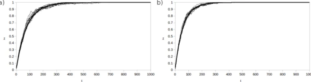
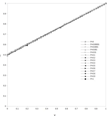
Figure 1: Time evolution of the proportion of payerszobtained from 10 simula-tions and the corresponding continuous solution (5) of the mean field differential equation (4) with a value of Θ0 given by equation (7) for ˆk = 5 andν = 0.02.
The values that define the Small-Network topology are: p= 0.1 andp= 1. The characteristic time of the population is given by equation (6) and depends on
p. For instance, it can be easily calculated thatTc≈77.52 forp= 0.1.
have the mean field equation:
d z
d t(t) = α ν(1−z(t)) (3)
In case of general networks, it is reasonable to start assuming that the ”time
scale” depends on both the average connectivity ˆk and the parameter p and
hence, to write:
d z
d t(t) = Θ0(ˆk, p)ν(1−z(t)) (4)
For instance, in the trivial case k= 0 in which each node is isolated we would
have Θ0(0, p) = 0. Starting from the initial conditionz(0) =ν we get:
z(t) = 1−(1−ν)e−νΘ0(ˆk,p)t (5)
For ˆk >0, the unique equilibrium point isz= 1 irrespectively of the value of
ν, meaning that the asymptotic population is formed exclusively by payers. The
main difference with respect to the case of propagation of epidemics (in which,
in the simplest case, the solution is a logistic curve) consists in the asymmetry
induced by the fact that, in case of infectious diseases the contagion acts just
from the infectious individuals to the susceptive ones and not vice-versa. The
rate at which the equilibrium point is approximated depends on the fraction of
the inspected nodes and on the structure of the network. Indeed, although the
time to achieve the equilibrium is infinite, it is still possible to get an estimate of
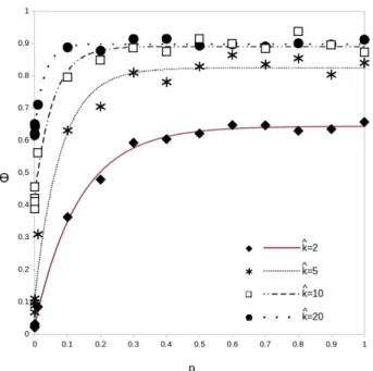
Figure 2: Fit of the diffusion rate Θ0 in terms of p for some values of ˆk: 2
(diamonds and continuous line), 5 (stars and dashed line), 10 (squares and dash-point line) and 20 (circles and point line). The total population, i.e. the number of nodes isN = 5000. For each simulation we get a value of Θ0. Each
point of the graph is obtained from the average of ten Θ0-values. As it can be
Table 1: Estimated value of the parameters of function (7) for different values of ˆk.
ˆ
k α β γ R-square
2 0.6435 0.6163 7.388 0.9982 5 0.8241 0.7126 12.79 0.9839 10 0.8906 0.4643 18.16 0.9845 20 0.8987 0.2679 32.71 0.9906
by the value of the ”characteristic time” [20], denoted asTc, which in the cases
where Θ0 is constant, e.g. for large values ofpand ˆk, is given by the inverse of
the absolute value of the eigenvalue of equation (4) :
Tc=
1
νΘ0(ˆk, p)
(6)
Concerning the dependence of Θ0 on ˆk and p, it can be inferred that it
is monotonically dependent on both variables. Moreover, if ˆk is fixed, it is
natural to assume that the derivative dΘ0
d p tends rapidly to zero aspincreases.
Conversely, if p is fixed, Θ0 goes from 0 (for ˆk = 0) to an asymptotic value
which is slightly increasing for increasing p. The functional dependence of Θ0
on ˆkandpcan only be determined from the simulations. The comparison of the
numerical data with the solutions of (4) for different values of ˆkandpallows to
obtain a good fitting with the function:
Θ0(ˆk, p) =α(ˆk)−β(ˆk)e−γ(ˆk)p (7)
where some values ofα(ˆk),β(ˆk),γ(ˆk) are given in table 1. Importantly enough,
theR-square of the fit is above 0.98 in all the considered cases. As it can be seen
in Fig.1, Θ0 increases very rapidly with pfor low values of pand it saturates
for p > 0.2. The saturation value depends on the average connectivity ˆk and
increases with it. This value is almost constant for any ˆk > 10 thus proving
that, in practice, the approximation (2) that we postulated for ˆk=N is valid
for any ”sufficiently connected” network. In Fig. 1 we show the time evolution
of payersz(t) obtained from simulations and by the mean field approximation
for large enough values ofp. The agreement is excellent for all times and for all
Remark 3.1
It has to be noted that the agreement between the mean field equation (4) and
the simulations is not adequate for lower p-values when the network becomes
almost regular, more precisely for p <0.1. Note that for the same parameter
setup used in Fig. 1, i.e. a network of size N = 5000, ˆk = 5 and ν = 0.02,
the number of initial payers (infectious agents) is very low, approximately 100,
that will be connected with low probability. This implies that initially, the
contagion rate of this behavior according with the probabilistic rule (1) will
be extraordinarily low. Therefore, it is expected that in these initial times, an
”anomalous” diffusion occurs [26, 9].
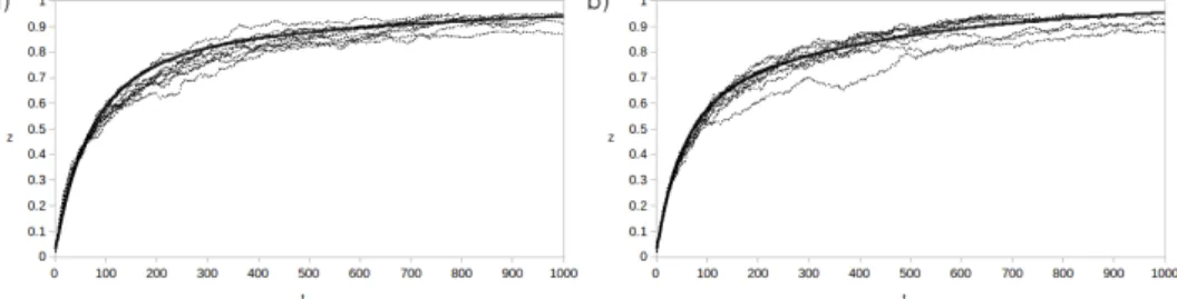
Figure 3: Time evolution of the proportion of payers zobtained from 10 simu-lations forp= 0 andp= 0.0001. For these low values ofpwe obtain a adequate fit using the mean field approximation described by equation (8) with a time-dependent diffusion rate. The function Θ is assumed to change accordingly to equation (9) with the fitting parameters given in Table 2. As in the previous figure, ˆk= 5 and ν= 0.02.
This means that a more accurate description of the ”contagion” by a mean
field approximation can be obtained if we substitute equation (4) by the
non-autonomous equation [14, 17]:
d z
d t(t) = Θ(ˆk, p;t)ν(1−z(t)) (8)
where the function Θ differs from the function Θ0 just during the transient
period. Figure 3 depicts the time evolution of the population of payers obtained
from the simulations and from non-autonomous mean field equation (8). As it
can be seen the agreement is good.
We have fitted Θ with simulations using the simple form:
where the values of parameters a, b and Θ0 can be found by comparison with
simulations. Note that the first term is significant only at initial times. This
transitory period depends onpand ˆkand tends to 0 when ptends to 1 and ˆk
increases. To our knowledge, there is not a complete theory about the spread
of information in complex networks in extreme situations as those occurred at
initial times in our model when the initial ”infectious nodes” are connected with
very low probability. Even the classic mean field approach is questioned in these
situations. We think that this subject is out of the scope of this work and it
will be discussed with some more detail in a forthcoming paper.
4
Discontinuos threshold rule
As stated in the introduction, local diffusion in social networks turns out to
be more complex than the continuous rule studied in the previous section. In
particular, threshold rules seem to mediate actively in the contagion of a large
group of social proceses. To take into account these cases, we define a willingness
of nodeito keep its current stateS1 (payer or evader) as:
W(i)S1→S1 =
N(i)S1
K(i) (10)
Similarly, the willingness to adopt the stateS2 is given by:
W(i)S1→S2 =
N(i)S2
K(i) (11)
As before, N(i)S1 and N(i)S2 are the number of neighbors of node i that are
in the statesS1 andS2, respectively andK(i)>0 is the connectivity of node
i. Note that W(i)S1→S2 = 1−W(i)S1→S1. The final decision of node iunder
the influence of its neighborhood depends on its personality that we take into
account by defining a parameter r∈[0,12], such that:
(i) The node i at state S1 will remain in this state if W(i)S1→S1 > r and
W(i)S1→S2 < r.
(ii) Nodeiwill change toS2ifW(i)S1→S1< randW(i)S1→S2> r.
(iii) The state of nodeiat the next time is taken randomly betweenS1andS2
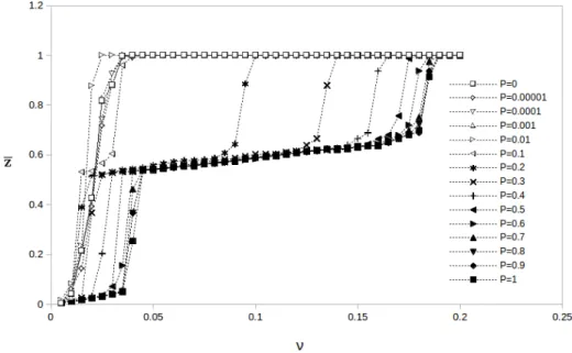
Figure 4: Equilibrium density of tax-payers ¯z as a function of the intensity of the initial inspections ν for different values of the network parameter p. A threshold contagion rule is used with a node personality given by r = 0.0. As before, the total population is N = 5000. In all simulations the initial population is formed entirely by tax-evaders. After the inspections, a fractionν
of tax-payers is initially present. All the points correspond to the average over 10 realizations taken after 104 time steps. Due to the lack of personality the
equilibrium population of payers increases linearly withν, fromz=1
2 forν = 0
Note that, the corresponding cases for12 < r≤1 can be obtained by
symme-try from theν-values ranging in the first half unit interval. As in the previous
model, those nodes that have been inspected adopt the state of payers forever.
The consideration of this threshold contagion rule modifies drastically the
asymptotic outcome of the population. The simplest situation is given by the
limit case r= 0 that corresponds to a population totally formed by indecisive
individuals. For this r-value, irrespective of the current state, a node chooses
randomly its next state. As Fig. 4 shows, the equilibrium population of
pay-ers ¯z increases linearly withν with a slope 1
2. This means that, independently
of p (and also of ˆk), half of the remaining population is converted to payers.
Nonetheless, the values of these parameterspand ˆk, affect the way the
equilib-rium population is attained.
The situation is more complicated for r > 0. For small intensity of
in-spections, the equilibrium population contains tax-evaders. The value of this
proportion depends on the intensityν, the structure of the networkpand also,
on the value of r. Figure 5 represents the equilibrium proportion of payers as
a function of the intensity of the inspections ν for different values of p when
r= 0.2 and the average connectivity is ˆk= 5. As it can be seen, three regimes
appear: for low values of ν, the population is almost fully formed by evaders,
irrespective of the value of p. This forms an upper branch in the bifurcation
diagram. If p > 0.1 then, the population remains stable in two intermediate
levels; a first one until the intensity of the inspections is lower thanν ≈0.04. A
second intermediate level, that corresponds to approximately half of the whole
population, exists for 0.04< ν < h(p), wherehis a function ofp. Forν > h(p)
the equilibrium population becomes tax-payer. As it can be observed, ifν >0.2
then, the asymptotic population is formed by tax-payers for all values ofp.
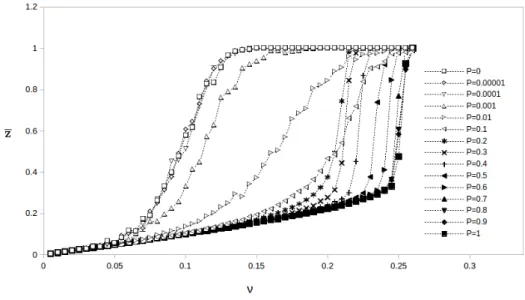
The intermediate branch disappears whenr= 0.5, i.e. if the threshold rule is
a pure majority rule (see Fig. 6). In this case, the interval of uncertainty where
WS1> randWS2 > rdoes not exist and, consequently this coexistence branch
is no longer present in the bifurcation diagram. The equilibrium population
of evaders decreases monotonically as the intensity of the inspections increases
untilν reaches a critical value that abruptly precipitates the evader asymptotic
Figure 5: As in the previous figure, the equilibrium value ¯z is plotted as a function ofν for different values ofp. The value of the node personalityr= 0.2. As before, the initial population is formed entirely by tax-evaders and, after inspections, a fraction ν of tax-payers is generated that remains forever. All the points correspond to the average over 25 realizations taken after 104 time
value can be approximately estimated from the maximum of the corresponding
standard deviation of the population for eachp-value.
Figure 6: As in Fig. 5 but with a personality r= 0.5. Now, contrary to what occurs in the previous figure 5 no intermediate branch appear for any value of
ν. As in the caser= 0.2 lower values ofpare more sensitive to inspections, i.e. the equilibrium population of payers achieve the upper branch for lower values ofν
For the limit ˆk =N, i.e. all nodes interact with each other, an analytical
solution of the mean field equation can be found (see Appendix 1). From this
solution the asymptotic behavior of the population in correspondence of any
pair (ν, r) can be derived (see Fig. 6). Whether a mean-field approximation
for any ˆk could be written in terms of some approximation of the Heaviside
functions, depending on ˆk and pas in the continuous contagion rule is under
investigation.
A ”mixed” rule, between the continuous rule and the discontinuous threshold
rule can also be considered. Two possibilities come to mind:
(1) Changing the rule expressed under (iii) of Sec.4 and assuming instead that
ifW(i)S1→S1 ≥r andW(i)S1→S2 ≥r, i.e. the uncertainty interval, then
the state of nodeiwill evolve according to probabilitiesP(i) that coincide
withW(i).
2 according to the continuous rule and byT(S1 →S2) the probability of
passing from state 1 to state 2 according to the threshold rule. Then, it
could be assumed that
P(S1→S2) =c C(S1→S2) + (1−c)T(S1→S2) (12)
for a fixed value ofc∈(0,1).
In the Appendix 2 we present the solution of the mean field approach that
corresponds to the mixed rule (1) for the limit casek=N. It can be appreciated
that, when compared with the discontinuous rule, the behaviour in this case is
simpler due to the absence of the uncertainty region (see Figures 7 and 8).
5
Discussion
The existence of interactions among the members of a society brings about a
social network where the nodes are individuals and the edges (links) represent
the relationships among nodes. The way a social network reacts to external
influences, e.g. inspections, depend mainly on their structure and the way
information is transmitted through the network, i.e. social contagion. In this
paper we have studied a toy model that considers that the individuals of a
population form a small world social network. We use the model of Watts and
Strogatz to tune the degree of randomness of the network from regular (p= 0)
to pure random network (p = 1). For each value of p, we have applied an
inspection strategy that consists in converting a fractionν of nodes that are
tax-evaders into tax-payers. We assume that inspected nodes are tax-payers forever
in the time scale of the population dynamics. We have also considered two
local contagion rules: continuous and discontinuous. For each parameter setup
we have applied both rules and we have confirmed that completely different
results are obtained. The equilibrium population for the continuous probabilistic
contagion rule is formed only by tax-payers, irrespectively of the intensityν of
the initial inspections and the structure of the network p. In contrast, when
the threshold rule is applied, the equilibrium population depends on both ν
and p. Besides, different willingness to change under the threshold rule gives
rise to distinct bifurcation diagrams as depicted in Figures 5 and 6. For the
growth rate Θ withpand the average connectivity ˆk. It has been proven that
the characteristic time to achieve the equilibrium population decreases inversely
with the intensity of inspection and increases withpand ˆkthat, ultimately, are
a measure of the characteristic path length of the network.
These results offer new alternatives to the authorities that fight tax evasion
and fraud. Knowing the topological properties of the social network allows
to estimate the network parameters p and ˆk, assuming to be of small world
type. With this knowledge, it is possible to apply an intensity of inspections to
achieve the optimal response with the lowest cost. For instance, if we discover
that the structure of the social network is compatible with a small world of
Watts-Strogatz with p= 0.2 and ˆk = 5 and we assume a threshold contagion
rule with a willingness to change of r = 0.2 then, the minimum intensity of
inspections that assure the lowest population of free riders is ν = 0.1. If the
willingness to change isr= 0.5, instead the intensity of inspections that assure
a lowest cost isν= 0.23. But even if in case of not having a complete certitude
about the structure of the network, the model provides a largest value of the
intensity of the inspections to get a complete eradication of free-riders, around
ν = 0.19 for r = 0.2 and ν = 0.26 for r = 0.5. In the extreme caser = 0, a
non-null population of evaders remains for everyν <1 (see Fig. 5. The absence
of personality requires greater efforts to fight tax-evasion.
We would like to end this discussion by making a short reference to the effect
of the choice of the inspected individuals in the population. In our model, all the
inspections have been carried out randomly, i.e. the nodes to be inspected have
been selected without any additional information. However, when the resources
are limited, the choice of the correct nodes to be inspected is a critical issue of
major relevance [27, 15]. It is true that when the network is homogeneous, as
the Small-World model, the preference in the inspection attending to the node
degree is not relevant since all the networks have the same average connectivity.
On the contrary, for inhomogeneous networks the way inspections are performed
could be decisive. Indeed, a preferential vaccination based on the connectivity
degree has been proven very useful to control the spread of epidemics on scale
Acknowledgements
Francisco Mu˜noz thanks the Mediterranean Office for Youth Program by the
mo-bility grant (MOY GRANT N+2010/024/01) in the Program Master in
Math-ematics and Mathematical engineering. Juan Carlos Nu˜no wishes to
acknowl-edge the European Erasmus staff mobility programmes. We are grateful to
Laura Navajas for checking the English of this manuscript. We also thank the
reviewers for their useful suggestions and remarks.
Appendix 1: Mean field approximation for the
threshold rule
For the limit case ˆk=N, i.e. all nodes interact with each other,
W(i)X→Y =y; W(i)Y→X=x+ν
we normalize the diffusion coefficient by changing the time scale and we consider
the different situations that may arise separately.
Let us assume that 0< r < 12 and the initial conditionz(0) =ν. For a given
value of pthe solution as a function of the initial condition ν and the value of
rreads:
(I) Ifν < rthen, equation (8) reduces to:
d z
d t(t) =ν−z(t) (13)
The solution of the corresponding Initial Value Problem (IVP) is : z(t) =
ν.
(II) Ifr < ν <1−2rthen,
d z
d t(t) =−z(t) +
1
2(1 +ν) (14)
In this case, the solution of the IVP is given by:
z(t) = 1
2((1 +ν) + (ν−1)e −t)
that tends asymptotically to the equilibrium solution: ¯z=1
Figure 7: Asymptotic behaviour of the population of payers as a function of the initial conditionz(0) =ν and the parameterr≤ 1
2 for a WS network with
ˆ
(III) Ifν >1−r then,
d z
d t(t) = 1−z (15)
and the solution of the IVP is:
z(t) = 1 + (ν−1)e−t
that approaches the equilibrium value ¯z= 1 asttends to infinity.
(IV) If 1−2r < ν < 1−r then, the population starts in a situation of uncertainty and, as in (II), the population is described by equation (14).
After some time, it switches to case (III) and the population is described
by (15). Consequently, the equilibrium value for this case coincides with
(III), i.e. ¯z= 1
Appendix 2: Mean field approximation for the
”mixed” rule
In this section, we present the analytical solution of the mean field equation
when ˆk=N for the mixed rule that considers a probabilistic transition in the
uncertainty interval, as described at the end of section 4.
In this case, the differential equations that result as a function of the relation
between the initial conditionν andrare:
1. If ν > rand 1−ν < rthen,
d z
d t(t) = 1−z(t)
2. If ν < rand 1−ν > rthen,
d z
d t(t) =−(z(t)−ν)
3. ifν > r and 1−ν > r as well as ifν < rand 1−ν < rthen,
d z
d t(t) =z(t) (1−z(t))−(1−z(t)) (z(t)−ν) =ν(1−z(t)) (16)
This means that, if we start fromν that is in the uncertainty region then,ν
is in the interval (r,1−r), assumingr < 1
Figure 8: Asymptotic behaviour of the population of payers as a function of the initial conditionz(0) =ν and the parameterr≤ 1
2 for a WS network with
ˆ
k=N for the mixed rule in the uncertainty interval (see main text). Note that the behaviour is symmetric with respect to the value r= 1
2. If compared with
for some time interval, by the (16), whose solution with the initial condition
z(0) =ν is:
z(t) = 1−(1−ν)e−ν t.
Therefore,z(t) is always increasing. In consequence, it will cross the value 1−r
at some time T and thus, leave the uncertainty region. From this instant on,
the ODE that describes the time evolution is:
d z
d t(t) = 1−z(t)
whose solution isz(t) = 1 +α e−t, whereαcan be found imposing thatz(T) = 1−r. In any case,z(t) will eventually tend to 1. Note that precisely, att=T
the derivative d zd t(t) jumps fromr ν to r.
Comparing this result with that obtained for the discontinuous rule, in the
”mixed case” we have simply that for ν < r, z(t) is constantly equal toν and
for ν > r then, z(t) tends to 1. As before, a symmetrical situation occurs for
r > 12. In conclusion, the pure threshold rule exhibits a richer behaviour than
the mixed rule, at least in the mean field approximation.
References
[1] Andrei, A.L., K. Comer and M. Koehler. An agent-based model of network
effects on tax compliance and evasion. Journal of Economic Psychology.
vol. 40, issue C, 119-133 (2014)
[2] B. Barzel and A.L. Barab´asi. Universality in network. Nature Physics 9,
673-681 (2013) doi:10.1038/nphys2741dynamics.
[3] Barash, V. The dynamics of social contagion. Doctoral Thesis (Faculty of
the Graduate School of Cornell University) (2011)
[4] Bloomquist K.M. A comparison of agent-based models of income
tax-evasion. Social Science Computer Review. Vol. 24 no. 4 411-425 (2006)
[5] Caldarelli, G. Scale free networks. Complex webs in nature and technology.
Oxford University Press (2007)
[6] Campbell, E. and M. Salath´e. Complex social contagion makes networks
[7] Centola, D. and M. Macy. Complex Contagions and the Weakness of Long
Ties. American Journal of Sociology, Vol. 113, No. 3, pp. 702-734
(Novem-ber 2007)
[8] D. Centola. The spread of behavior in an online social network. Science,
329, 1194 (2010)
[9] Dmitry S. Novikov, Els Fieremans, Jens H. Jensen and Joseph A.
Helpern. Random walk with barriers. Nat Phys. 7(6): 508-514 (2011)
doi:10.1038/nphys1936
[10] Jackson M.E. and D. L´opez-Pintado. Diffusion and contagion in networks
with heterogeneous agents and homophily. Network Science / Volume 1 /
Issue 01 / April 2013, pp 49 - 67 DOI: 10.1017/nws.2012.7
[11] Falk, A. and U. Fischbacher. ”Crime” in the lab-detecting social interaction.
European Economic Review 46 (2002) 859 ˆu 869
[12] Granovetter, M.: Threshold models of collective behavior. The American
Journal of Sociology (6), 1420-1443 (May 1978) DOI 10.2307/2778111
[13] Gintis, H., S. Bowles, R. Boyd and E. Fehrd. Explaining altruistic behavior
in humans. Evolution and Human Behavior 24, 153-172 (2003)
[14] Peter E. Kloeden, Christian P¨otzsche (Eds.) Nonautonomous Dynamical
Systems in the Life Sciences. Lecture Notes in Mathematics. Springer
In-ternational Publishing, Switzerland (2013)
[15] Kuhlman, C.J., V.S. Anil Kumar, M V. Marathe, S.S. Ravi and D. J.
Rosenkrantz. Finding Critical Nodes for Inhibiting Diffusion of Complex
Contagions in Social Networks. J.L. Balc´azar et al. (Eds.): ECML PKDD
2010, Part II, LNAI 6322, pp. 111-127, Springer-Verlag (2010)
[16] Hagberg, A.A., D.A. Schult and P.J. Swart. Exploring network structure,
dynamics, and function using Networkx. Proceedings of the 7th Python in
Science Conference (SciPy) (2008)
[17] Hallam, T.G. and C.E. Clark. Non-autonomous logistic equations as
mod-els of populations in a deteriorating environment. Journal of Theoretical
[18] Hodas, N.O. and K. Lerman. The simple rules of social contagion. Scientific
Reports,4, 4343 DOI: doi:10.1038/srep04343 (2014)
[19] Llacer, T., F.J. Miguel, J.A. Noguera and E. Tapia. An agent-based model
of tax compliance: an application to the Spanish case. Advs. Complex Syst.
16, 1350007 DOI: 10.1142/S0219525913500070 (2013)
[20] Llor´ens, M. J. C. Nu˜no, Y. Rodr´ıguez, E. Mel´endez-Hevia and F. Montero.
Generalization of the Theory of Transition Times in Metabolic Pathways:
A Geometrical Approach. Biophysical Journal Volume 77, 23-36 (1999)
[21] Pastor-Satorras, R. and A. Vespignani. Immunization of complex networks.
Phys. Rev. E 65, 036104 (2002).
[22] Perc, M., K. Donnay and D. Helbing. Understanding Recurrent Crime
as System-Immanent Collective Behavior. PLoS ONE 8(10): e76063.
doi:10.1371/ journal.pone.0076063 (2013)
[23] Pickhardt, M. and A. Prinz. Behavioral dynamics of tax evasion ˆu A survey.
Journal of Economic Psychology 40, 1ˆu19 (2014)
[24] Shakarian P., Sean Eyre and Damon Paulo. A Scalable Heuristic for Viral
Marketing Under the Tipping Model. arXiv:1309.2963v1 [cs.SI] 11 Sep 2013
[25] Schelling, T.C. Micromotives and Macrobehavior. W.W. Norton and Co.
(1978)
[26] Schweitzer F, Mach R. The Epidemics of Donations: Logistic Growth
and Power-Laws. PLoS ONE 3(1): e1458 (2008) doi:10.1371/
jour-nal.pone.0001458
[27] Valente, T. W. Network interventions. Science. 337, 49 (2012). DOI:
10.1126/science.1217330
[28] Vespignani, A. Modelling dynamical processes in complex socio-technical
systems. Nat. Phys., VOL 8, JANUARY 2012.
[29] Watts, D.J. and S.H. Strogatz. Collective dynamics of small-world
[30] Watts, D.J. Six degrees: the science of a connected age. Random House:
London, UK (2003)
[31] Zaklan G., F.W.S. Limab and Frank Westerhoff. Controlling tax evasion
fluctuations. Physica A 387, 5857-5861 (2008)
[32] Zaklan, G., F. Westerhoff and D. Stauffer. Analysing tax evasion dynamics
via de Ising model. Journal of Economic of Coordination and Interaction,