TITULO 2D Eulerian-Eulerian shocked particle-laden flows : normal shockwave interaction with a cloud of particles

Proyecto Fin de Carrera

2D Eulerian-Eulerian Shocked Particle-Laden

Flows: Normal Shockwave interaction with a

Cloud of Particles.

Author:

Alfonso de las Heras Mu˜noz

Advisor: Dr. Gustaaf Jacobs Dr. Sean Davis

A thesis submitted in fulfilment of the requirements for the Master’s of Industrial Engineering

in

Department of Aerospace Engineering San Diego State University

Departamento de Ingenier´ıa Energ´etica y Fluidodin´amica Universidad de Valladolid

i

´

ii

Abstract:

The 2D Eulerian-Eulerian model is implemented in a high-speed particle-laden flow for

the first time to elucidate the interaction between a right-running shock and a cloud of particles. The Eulerian particle phase is modeled as a compressible fluid, which reduces

the computational cost of modeling large amount of particles. Source terms in the Eulerian governing equations allow for the tranfer of momentum and energy between the phases.

Second moments provide information about the inertial effects and create a non-linear system of equations. High-order, finite difference, WENO schemes are able to capture the

Acknowledgements

First, I would like to thank Mª Teresa for giving me the oportunity to come to San

Diego for this year as well as to Gustaaf Jacobs for guiding me throughout this project.

I would also like to thank Sean Davis for all the time he spent helping me with mmy

work.

I would want to remember all the people I shared with this experience, specially those

who came with me from Valladolid, Eduardo and Ignacio, as well as Wouter, because

they have been like my family along this year; my roomates Francesco and Vincenzo for

all the time we shared together and my labmates because they were always willing to

help me out.

Last but not least, I want to heartily thank my family; my parents, Constantino and

Blanca, and my sister, Cristina; for all the support and understanding they gave me.

Contents

Abstract ii

Acknowledgements iii

Contents iv

List of Figures v

List of Tables vi

Symbols vii

1 Introduction 1

2 Governing Equations 3

2.1 Carrier Phase . . . 3

2.2 Disperse Phase . . . 5

2.3 Two-Way Coupling . . . 12

3 Numerical Methods 13 3.1 Averaging . . . 13

3.2 WENO method . . . 14

3.3 Temporal Stability . . . 16

4 Moving Normal Shockwave 17 4.1 Setup . . . 18

Boundary Conditions. . . 18

4.2 Results. . . 19

4.2.1 Carrier Phase . . . 22

4.2.2 Disperse Phase . . . 24

5 Conclusions and Future Work 25

List of Figures

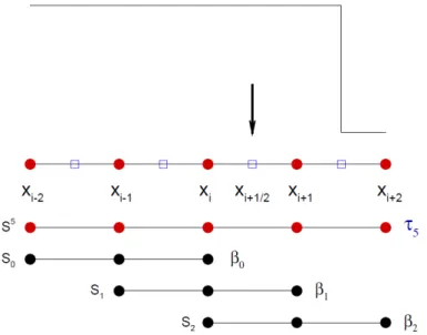
3.1 Discontinuity between cell boundariesxi+1 and xi+2. xi+1/2 represents a cell center. WENO scheme 5-points Stencil is S5. Three 3-points

subs-tencil are (S0, S1, S2). . . 15

4.1 Carrier Phase Setup . . . 17

4.2 Particle Phase Setup . . . 17

4.3 Fluid velocity in x direction, at the time 0.14s . . . 19

4.4 Fluid pressure, at the time 0.14s . . . 19

4.5 Fluid temperature, at the time 0.14s . . . 20

4.6 Fluid density, at the time 0.14s . . . 20

4.7 Fluid velocity in y direction, at the time 0.14s . . . 21

4.8 Streamlines around the particle cloud, at the time 0.14s . . . 21

4.9 Particle density number, at the time 0.14s . . . 22

4.10 Particle velocity in x direction, at the time 0.14s . . . 23

4.11 Particle velocity in y direction, at the time 0.14s . . . 23

4.12 Particle temperature, at the time 0.14s . . . 24

List of Tables

4.1 Domain setup. . . 18 4.2 Carrier Phase initial conditions. . . 18 4.3 Disperse Phase initial conditions. . . 18

Symbols

x, y Position

xp Particle position

ρ Fluid density

u Fluid velocity in x

v Fluid velocity in y

T emp Fluid temperature

p Fluid pressure

H Enthalpy

c Sound speed

M Mach number

γ Ratio gas capacities

β Ratio of particle heat capacity to fluid heat capacity at constant pressure

τp Particle relaxation time constant

τT Particle thermal relaxation time constant

ρf Reference density

Uf Reference velocity in x

Vf Reference velocity in y

Mf Reference Mach number

Lf x Reference length in x

Lf y Reference length in y

Tf Reference Temperature

Mp Mass of a single particle

φ Particle number density

up Particle velocity in x

vp Particle velocity in y

Symbols viii

θ Particle temperature

W Fine-grained phase-space density function

δ Dirac delta function

H∆ Kernel function

∗ Dimensional variables

Chapter 1

Introduction

Particle-Laden Flows are composed by two phases. The Euler Phase or also named

Carrier Phase which is usually a gas and the Particle Phase or Disperse Phase, which is

composed by small, immiscible particles in suspension inside the Carrier Phase. These

phases are together and mixed. Particle-Laden flows are present in such environments as

volcanic eruptions, pollution dispersion in the atmosphere or fluidization in combustion

processes. Some industrial applications can be the aerosol deposition in spray

medica-tion, turbulent mixing of liquid fuel particles with air in an automobile’s engine or fuel

spray in a gas turbine. [1], [5].

This problem has been traditionally faced with a classical Euler approach for the Carrier

Phase, using the Navier-Stokes equations which focuses on an specific location or Control

Volume through which the fluid passes by; and a Lagrangian approach for the Disperse

Phase, where the observer follows an individual fluid parcel as it moves through space

and time. This is called the E-L model. E-L model is explained in [3].

Since the Particles are usually considered spherical and light enough to behave as a

fluid, an Eulerian treatment of the disperse Phase is sensible. Secondly, when the

por-blem requires to solve a large amount of particles, Lagrangian frame become a very

computationally expensive method. In this thesis, and Eulerian Eulerian, E-E model

is developed and, as we will see, the Euler this approach for the problem, which

basi-cally means modelling the particles as a second fluid inside the Carrier Phase, is a good

method as well.

An analysis of the results are presented, using a WENO method to solve it. This method

is very suitable for the problem beacuse of the high accuracy in smooth areas providing

the neccessary dissipation for capturing shockwaves. Further information about WENO

schemes will be provided by [3],[4].

Chapter 1. Introduction 2

First, we introduce the physical model: The Carrier Phase, the Disperse Phase and

the coupling between them. In Chapter 3, the numerical methods used to solve the

problem will be discussed. In section Chapter 4, the problem is solved, setting a Normal

Shockwave interacting with a rectangular cloud of particles. Plots representing the main

variables of the problem are shown and results are discussed. Finally, in section Chapter

Chapter 2

Governing Equations

2.1

Carrier Phase

The following assumptions are made to derive the Euler equations:

• The fluid is Newtonian.

•The fluid is continuous, so the smallest length scale of motion of the fluid is very large compared with the molecular motion.

• It is a convection dominated flow, hence the inviscid Euler equations are used.

•The fluid is considered an idel gas. Intermolecular forces are negligible and the equation of state is given by the ideal gas law.

The first step is to non-dimensionalize the equations that are given. We normalize them

using a reference length Lf, reference density ρf, reference velocity Uf and Vf and

reference temperatureTf. The non-dimensional variables are the following:

x = x

∗

Lf x

, y = y

∗

Lf y

, (2.1)

u = u

∗

U_f∗, v =

v∗

V_f∗, (2.2)

ρ = ρ

∗

ρ∗_f, T =

T∗

T_f∗, (2.3)

p = p

∗

ρ∗_fU_f∗2, t =

t∗U_f∗

L∗_f (2.4)

. From the non-dimensional variables, we can build the Euler equations,

∂Qf

∂t + ∂Ff

∂x + ∂Gf

∂y = 0 (2.5)

Chapter 2. Governing Equations 4

Qf =

       ρ ρu ρv E       

, Ff =

       ρu

ρu2+p ρuv

(E+p)u       

, Gf =

       ρv ρuv

ρv2+p

(E+p)v        (2.6)

Where Q contains the conservative variables, while F and G are the fluxes in x and y

respectively. If we apply the Chain Rule, we obtain the characteristic form

∂Qf

∂t +Af ∂Qf

∂x +Bf ∂Qf

∂y = 0, (2.7)

whereAf and Bf are the Jacobian Matrix of the system in x and y dimensions. In the

x-direction, the jacobian matrix is

Af =

      

0 1 0 0

1

2[(γ−3)u2+ (γ−1)v2] (3−γ)u −(γ−1)v γ−1

−uv v u 0

γuE+ (γ−1)u(u2+v2) γE−γ−₂1(v2+ 3u2) −(γ−1)uv γu        , (2.8)

and the corresponding eigenvalues and eigenvectors associated,

λ1=u−c , λ2=u , λ3=u , λ4=u+c, (2.9)

r1 =

       1

u−c v

H−uc       

, r2 =

       1 u v 1 2(u

2_+v2₎

      

, r3 =

       0 0 1 v       

, r4 =

       1

u+c

v

H+uc        (2.10) .

Similarly in the y-direction,

Bf =

      

0 0 1 0

−uv v u 0

1

2[(γ−1)u

2_{+ (γ−3)v}2_{] −(γ−1)u (3−γ)v γ−1}

−γuE+ (γ−1)v(u2+v2) −(γ−1)uv γE−γ−₂1(u2+ 3v2) γv        , (2.11)

and the corresponding eigenvalues and eigenvectors

Chapter 2. Governing Equations 5

r1=

       1 u

v−c H−vc

      

, r2=

       1 u v 1 2(u

2_+v2₎

      

, r3 =

       0 1 0 u       

, r4=

       1 u

v+c

H+vc        (2.13) .

In order to close the system of equations, the Stagnation Energy equation is used

E = p γ−1 +

1 2(u

2_+v2_{), (2.14)}

along the Ideal gas law.

p= ρT

γ (2.15)

2.2

Disperse Phase

The Particle-Phase equations in the Eulerian frame are derived from the Lagrangian

equations of the position vector xP, the velocity vectorvP and the temperature θP of a

single particle. uis the fluid velocity vector andT corresponds to the fluid temperature.

More detailed explanation is shown in [2].

dxP

dt =vP (2.16)

dvP

dt = 1 τP

(u−vP) (2.17)

dθP

dt = 1 τT

(T −θP) (2.18)

In order to implement the Eulerian paticle phase equations, we need to derive a

conti-nuity variable. We use the Number Density Functionφ.

A fine-grained phase-space density function is defined as,

W(x, v, θ, t) =δ[x−xP(t)]δ[v−vP(t)]δ[θ−θP(t)] (2.19)

The fine grained phase-space densuty function verifies the Liouville equation in the phase

space

∂W ∂t +

∂viW

∂xi

− ∂

∂vi

[(vi−ui) τP

W]− ∂

∂θ[

(θ−T) τP

W] = 0 (2.20)

A spatial filtering operation is applied,

¯ f(x) =

Z

Chapter 2. Governing Equations 6

where ¯f(x) is the filtered value of f(x), H∆ the Kernel Function and ∆ the size of the

filter. This size is chosen small, in order to avoid subgrid-scale fluctuations. The filtered

Liouvulle equation is

∂W¯ ∂t +

∂viW¯

∂xi

− ∂

∂vi

[(vi−ui) τP

¯ W]− ∂

∂θ[

(θ−T) τP

¯

W] = 0, (2.22)

where ¯W is a coarse-grained fucntion with all the properties of a probability density

function when the KernelH∆ is positive. The Number Density,φ, the Eulerian velocity

and Eulerian temperature are obtained in terms of ¯W as follows,

¯ φ=

Z ¯

W(x, v, θ, t)dvdθ, (2.23)

¯ vi=

1 ¯ φ

Z

viW¯(x, v, θ, t)dvdθ, (2.24)

¯ θ= 1_¯

φ Z

θW¯(x, v, θ, t)dvdθ. (2.25)

Using these equations and the definitions we obtain the governing equations for the

Particle Phase:

∂φ¯ ∂t +

∂φ¯v¯i

∂xi

= 0, (2.26)

∂φ¯v¯i

∂t + ∂φv¯ ivj

∂xj

= 1 τP

¯

φ(ui−v¯i), (2.27)

∂φ¯θ¯ ∂t +

∂φ¯θv¯i

∂xi

= 1 τT

¯

φ(T−θ),¯ (2.28)

∂φv¯ ivj

∂t +

∂φv¯ ivjv_k

∂xk

= 1 τP

¯

φ(uiv¯j+ ¯viuj−2vivj), (2.29)

∂φθv¯ i

∂t +

∂φθv¯ ivk

∂xk

= 1 τP

¯

φ(uiθ¯−θvj) +

1 τT

¯

φ(Tv¯i−θvj). (2.30)

In order to close the system of equations, we model the third-order moments

approxi-mating:

vivjv_k−vjvkv¯i−vivjv¯k−vivkv¯j+ 2 ¯viv¯jv¯k≈0, (2.31)

θvjv_k−θvkv¯i−θvjv¯k−vivkθ¯+ 2 ¯viv¯kθ¯≈0. (2.32)

For the 2D case, we introduce the sub-grid scale particle stress, σij, and the sub-grid

scale particle heat flux,qq_i. These terms capture information about the inertial effects,

σij = vivj −v¯iv¯j, (2.33)

Chapter 2. Governing Equations 7

Once we have modelled the particle phase in the Eulerian frame, we can use the same

governing equation as in the carrier phase, introducing the particle variables described

before: ∂QP ∂t + ∂FP ∂x + ∂GP

∂y = 0 (2.35)

where Q contains the conservative variables φ,e u_fP, v_fP, θ,e σ_uu, σ_vv, σ_uv, qq_u, qq_v while F and G are the fluxes in x and y direction respectively,

QP =

                    e φ e φufP

e φv_fP

e φθe

e

φ(σuu+ufP

2

)

e

φ(σuv+ufPvfP) e

φ(σvv+vfP

2

)

e

φ(qq_u + θe f uP)

e

φ(qq_v + θev_fP)                     =                     Q1 Q2 Q3 Q4 Q5 Q6 Q7 Q8 Q9                     , (2.36)

FP =

                    Q2 Q5 Q6 Q8

−2Q₂3/Q12+ 3Q2Q5/Q1

2Q₂Q6/Q1+Q3Q5/Q1−2Q22Q3/Q2₁

Q2Q7/Q1+ 2Q3Q6/Q1−2Q2Q23/Q21

Q4Q5/Q1+ 2Q2Q8/Q1−2Q22Q4/Q2₁

Q4Q6/Q12+Q2Q9/Q1+Q3Q8/Q1−2Q2Q3Q4/Q12

                    , (2.37)

GP =

                    Q3 Q6 Q7 Q9

2Q₂Q6/Q1+Q3Q5/Q1−2Q22Q3/Q1

Q2Q7/Q1+ 2Q3Q6/Q1−2Q2Q23/Q1

−2Q₃3/Q12+ 3Q3Q7/Q1

Q4Q6/Q12+Q2Q9/Q1+Q3Q8/Q1−2Q2Q3Q4/Q12

Q4Q7/Q1+ 2Q3Q9/Q1−2Q23Q4/Q21

Chapter 2. Governing Equations 8

Applying the chain rule, the characteristic form is derived,

∂QP ∂t + ∂FP ∂QP ∂QP ∂x + ∂GP ∂QP ∂QP

∂y = 0, (2.39)

where AP = _∂Q∂FP_P and BP = ∂G_∂QP_P are the Jacobian matrix of the system in the x and y

direction respectively,

Ap=

                  

0 1 0 0 0 0 0 0 0

0 0 0 0 1 0 0 0 0

0 0 0 0 0 1 0 0 0

0 0 0 0 0 0 0 1 0

f

up 2

−3σuufup 3σuu−3ufp

2

0 0 3u_fp 0 0 0 0

e

vpfup

2

−2σuvufp−σuuvep 2σuv−2ufpvep σuu−ufp

2

0 v_ep 2fup 0 0 0 f

upv_ep2−2σuvv_ep−σvv_fup σvv−v_ep2 2σuv−2_fupv_ep 0 0 2v_ep _fup 0 0

e

θ_fup2−2qqufup−σuuθe 2qqu−2θefup 0 σuu−ufp

2

e

θ 0 0 2u_fp 0

e

θu_fPvfP−qquvep−σuvθe−qqvfup qqv−θevep qqu−θefup σuv−ufpvep 0 θe 0 vep fup                    , (2.40)

and the eigenvalues and eigenvectors associated,

λ1=ufP −

√

3σuu, λ2=ufP +

√

3σuu,

λ3=ufP, λ4=ufP, λ5=ufP, λ6=ufP +

√

σuu, λ7 =ufP +

√

σuu,

λ8=ufP −

√

σuu, λ9 =ufP −

√

σuu,

r1 =

                     1 f uP −

√

3σuu f

vP

√

σuu−σuv

√

3

√

σuu

e

θ√σuu−qqu

√

3

√

σuu

(u_fP −

√

3σuu)2

(ufP−

√

3σuu)(vfP

√

σuu−σuv

√

3)

√

σuu

σuuσvv+σuuvfP

2

+2σuv2−2vfPσuv

√

3σuu

σuu

(eθ

√

σuu−qqu

√

3)(ufP−

√

3σuu)

√

σuu

2qq_uσuv+qqvσuu+vfPσuueθ−qquvfP

√

3σuu−eθσuv

√

3σuu

Chapter 2. Governing Equations 9

r2 =

                     1 f uP +

√

3σuu σuv

√

3+vfP

√ σuu √ σuu qqu √

3+eθ

√

σuu

√

σuu

(u_fP +

√

3σuu)2

(ufP+

√

3σuu)(vfP

√

σuu+σuv

√

3)

√

σuu

σuuσvv+σuuvfP

2

+2σuv2+2vfPσuv

√

3σuu

σuu

(θe

√

σuu+qqu

√

3)(ufP+

√

3σuu)

√

σuu

2qq_uσuv+qqvσuu+vfPσuuθe+qquvfP

√

3σuu+θσe uv

√

3σuu

σuu                      , (2.42)

r3=

                    0 0 0 0 0 0 1 0 0                    

, r4 =

                    1 f uP f vP e θ f uP2

f uPvfP

0

e θu_fP

0                    

, r5 =

                    0 0 0 0 0 0 0 0 1                     , (2.43)

r6 =

                     0 0 1 −(qqu+θe

√

σuu)

σuv+vfP

√

σuu

0

f uP +

√

σuu

2(σuv+vfP

√

σuu)

√

σuu

−(qqu+θe

√

σuu)(ufP+

√

σuu)

σuv+vfP

√ σuu 0                     

, r7=

                    0 0 1 0 0 f uP +

√

σuu

2(σuv+vfP

√

σuu)

√

σuu

0

qqu+θe

√ σuu √ σuu                     , (2.44)

r8 =

                     0 0 1 −(qqu−θe

√

σuu)

σuv+vfP

√

σuu

0

f uP −

√

σuu

−2(σuv−vfP

√

σuu)

√

σuu

−(qqu−θe

√

σuu)(ufP−

√

σuu)

σuv−vfP

√ σuu 0                     

, r9=

                    0 0 1 0 0 f uP −

√

σuu

−2(σuv−vfP

√

σuu)

√

σuu

0 −(qq_u−eθ

√

σuu)

Chapter 2. Governing Equations 10

In y direction,

Bp=

                  

0 0 1 0 0 0 0 0 0

0 0 0 0 0 1 0 0 0

0 0 0 0 0 0 1 0 0

0 0 0 0 0 0 0 0 1

e

vpfup

2

−2σuvfup−σuuvep 2σuv−2ufpvep σuu−ufp

2

0 v_ep 2fup 0 0 0 f

upv_ep2−2σuvv_ep−σvv_fup σvv−v_ep2 2σuv−2_fupv_ep 0 0 2v_ep _fup 0 0

e

vp3−3σvvv_ep 0 3σvv−3v_ep2 0 0 0 3v_ep 0 0

e

θ_fupvep−qquvep−σuvθe−qqvfup qqv−θevep qqu−θefup σuv−ufpvep

2

0 θe 0 v_ep ufp e

θv_ep2−2qqvvep−σvvθe 0 2qqv−2θevep σvv−vep

2

0 0 eθ 0 2v_ep

                   , (2.46)

and the eigenvalues and eigenvectors associated,

λ1=vfP −

√

3σvv, λ2 =vfP +

√

3σvv,

λ3=vfP, λ4 =vfP, λ5=vfP, λ6=vfP +

√

σvv, λ7 =vfP +

√

σvv,

λ8=vfP −

√

σvv, λ9 =vfP −

√

σvv,

r1 =

                     1 f uP √

σvv−σuv

√

3

√

σvv

f vP −

√

3σvv e

θ√σvv−qqv

√

3

√

σvv

σuuσvv+σvvufP

2_+2σ

uv2−2ufPσuv

√

3σvv

σvv

(vfP−

√

3σvv)(ufP

√

σvv−σuv

√

3)

√

σvv

(v_fP −

√

3σvv)

2

2qqvσuv+qquσvv+ufPσvvθe−qqvufP

√

3σvv−θσe uv

√

3σvv

σvv

(θe

√

σvv−qqv

√

3)(vfP−

√

3σvv)

√ σvv                      , (2.47)

r2 =

                     1 σuv √

3+ufP

√

σvv

√

σvv

f vP +

√

3σvv qqv

√

3+θe

√

σvv

√

σvv

σuuσvv+σvvufP

2_+2σ

uv2+2ufPσuv

√

3σvv

σvv

(vfP+

√

3σvv)(ufP

√

σvv+σuv

√

3)

√

σvv

(v_fP +

√

3σvv)

2

2qqvσuv+qquσvv+ufPσvvθe+qqvufP

√

3σvv+θσe uv

√

3σvv

σvv

(θe

√

σvv+qqv

√

3)(vfP+

√

3σvv)

Chapter 2. Governing Equations 11

r3=

                    0 0 0 0 1 0 0 0 0                    

, r4 =

                    1 f uP f vP e θ 0 f uPvfP

f vP2

0

e θv_fP

                   

, r5 =

                    0 0 0 0 0 0 0 1 0                     , (2.49)

r6=

                     0 1 0 −(qqv+eθ

√

σvv)

σuv+ufP

√

σvv

2(σuv+ufP

√

σvv)

√

σvv

f vP +

√

σvv

0

0 −(qqv+eθ

√

σvv)(vfP+

√

σvv)

σuv+ufP

√ σvv                     

, r7 =

                    0 1 0 0

2(σuv+ufP

√

σvv)

√

σvv

f vP +

√

σvv

0

qqv+θe

√ σvv √ σvv 0                     , (2.50)

r8=

                     0 1 0 −(qqv−eθ

√

σvv)

σuv+ufP

√

σvv

−2(σuv−ufP

√

σvv)

√

σvv

f vP −

√

σvv

0

0 −(qq_v−eθ

√

σvv)(vfP−

√

σvv)

σuv−ufP

√ σvv                     

, r9=

                    0 1 0 0 −2(σuv−ufP

√

σvv)

√

σvv

f vP −

√

σvv

0 −(qq_v−θe

√

σvv)

Chapter 2. Governing Equations 12

2.3

Two-Way Coupling

We couple the phases by including a Source Term which accounts for the interaction

between the Carrier Phase and the Disperse Phase in the Fluid governing equations as

well as in the Particle governing equations. A momentum and energy tansfer occurs

between the phases. Because we are working with immiscible fluids, no mass transfer is

observed. The fluid source terms are,

Sf =

       0

mPφe

τP (ufP −u)

mPφe

τP (vfP −v)

βmPφe

(γ−1)M2

fτT(

e

θ−T) +mPφe

τP (σuu+ufP

2₊

f

uPu) +mP e φ

τP (σvv+vfP

2₊

f vPv)

       , (2.52)

and particle source terms are,

SP =

                     0 e φ

τP(u−ufP)

e φ

τP(v−vfP)

e φ

τT(T−θ)e

e φ τP(ufP

2₋

f

uPu+σuu)

−φe

τP(2σuv−uvfP −vufP + 2ufPvfP)

e φ τP(vfP

2₋

f

vPv+σvv)

−φe

τT(qqu−TufP +θeufP +θevfP)−

e φ

τP(qqu−eθu+θeufP +θevfP)

−φe

τT(qqv−TvfP +θeufP +eθvfP)−

e φ

τP(qqv−eθv+θeufP +θevfP)                      . (2.53)

The fully-coupled E-E model can be written as ,

∂Qf

∂t + ∂Ff

∂x + ∂Gf

∂y =Sf, (2.54)

∂QP

∂t + ∂FP

∂x + ∂GP

Chapter 3

Numerical Methods

3.1

Averaging

The first step in discretizing the governing equations is to linearize the non-linear

Ja-cobian matrix of the hyperbolic problem. Roe Averaging is used in the Eulerian phase

over the primitive variables to obtain a linear Jacobian:

ˆ u_i−1

2 =

√

ρi−1ui−1+

√

ρiui

√

ρi−1+

√

ρi

, (3.1)

ˆ v_i−1

2 =

√

ρi−1vi−1+

√

ρivi

√

ρi−1+

√

ρi

, (3.2)

ˆ H_i−1

2 =

√

ρi−1Hi−1+

√

ρiHi

√

ρi−1+

√

ρi

= (Ei−1+pi−1)/

√

ρi−1+ (Ei+pi)/

√

ρi

√

ρi−1+

√

ρi

, (3.3)

ˆ c=

r

(γ−1)( ˆH− 1

2uˆ

2_{). (3.4)}

Whereui−1is the velocity in x evaluated in the cell before,uiis the velocity in x evaluated

in the cell after and ˆu_i−1

2 is the averaged velocity in x, evaluated in the cell boundaries

between the two cells previously cited. The same occurs for the other variables.

Simple Averaging is used in the Particle Phase,

ˆ q_i−1

2 =

1

2(qi−1+qi), (3.5)

where ˆq_i−1

2 represents the primitive variables

e

φ, _fup, vep, θ,e fup

2

, u_gpvp, vep

2_,

g θup, θvf_p explained in Chapter 2 and evaluated in the cell boundary.

Chapter 3. Numerical Methods 14

3.2

WENO method

A Weight Esentially Non Oscillatory Conservative Finite Difference Scheme (WENO

Scheme) is suitable for this problem because it provides high accuracy in smooth areas,

good resolution around discontinuities and the necessary dissipation for shock capturing.

More information about WENO scheme is provided by [3] and [4].

An uniform grid is defined by the pointsxi =i∆x, i=0,...,N, called cell centers and the

cell boundaries are given byx_i+1

2 =xi+

∆x

2 where ∆xis the uniform grid spacing.

The discretization yields a system of ordinary differential equations,

dui(t)

dt =− ∂f ∂x x=xi

i= 0, ..., N, (3.6)

where ui(t) is the numercial approximation to the point value u(xi, t). We define the

numerical flux function as h(x). The conservative property of the spatial discretization

is obtained by this function,

f(x) = 1 ∆x

Z x+∆x

x−∆x

h(ξ)dξ, (3.7)

and the spatial derivative in 3.6is expressed by a conservative finite-difference formula

in the cell boundaries,

dui(t)

dt = 1 ∆x(hi+12

−h_i−1

2) (3.8)

A high order polinomial interpolation over h(x), using the known values of f inxi, is

used to determine this formula. The fifth order WENO scheme uses a 5 points stencil,

S5, composed of three 3-points stencil, S0, S1, S2, shown in Fig. 3.1. The fifth order

approximation ˆf_i±1

2 is built through a convex combination of the interpolated values

ˆ f_i±1

2,

ˆ f_i±1

2 =

2

X

k=0

ωz_kfˆk(xi±

1

2), (3.9)

where

ˆ f_ik_±1

2

=

2

X

k=0

ckjfi−k+j, i= 0, ..., N, (3.10)

and ckj are the Lagrangian interpolation coefficients, which depend on the parameter

k. This convex combination is made by weighing the different solutions obtained with

the sub-stencils. The WENO weights are defined as

ωz_k= α

z k

P2

l=0αkz

, ωz_k= dk βz k

Chapter 3. Numerical Methods 15

Figure 3.1: Discontinuity between cell boundariesxi+1 and xi+2. xi+1/2 represents

a cell center. WENO scheme 5-points Stencil is S5. Three 3-points substencil are

(S0, S1, S2).

where d0= ₁₀3, d1 = 3₅, d2 = ₁₀1 are the ideal weights and they generate a central

upwind fifth order scheme for the 5-points stencil. The weights are also a function of the

smoothness indicator given byβk, which measures the regularity of the kth polynomial

approximation.

If the smoothness indicators are close to one, the substencil weights are close to the

ideal weights. However, if Sk contains a discontinuity, βk is O(1) and the

correspond-ing weight, ωk, is relatively small compared with the other weights. Because of the

lower weighting, the influence of the polynomial approximation ofh_i±1

2 taken across the

discontinuity is dismished in the global solution up to the point, making the scheme

Chapter 3. Numerical Methods 16

3.3

Temporal Stability

The Courant-Friedrichs-Lewy condition, CFL condition is necessary in order to assure

the stability and convergence of the method,

∆t= CF L∗min(∆x,∆y)

max(λfxλfy)

, (3.12)

where ∆t is the time step, λ are the eigenvalues of the carrier phase in the x and y

dimensions and ∆x,∆y are the uniform grid spacing in the x and y dimensions

respec-tively. A RK3 scheme is used to update the time step so we obtain more stability than

Chapter 4

Moving Normal Shockwave

Figure 4.1: Carrier Phase Setup

Figure 4.2: Particle Phase Setup

Chapter 4. Moving Normal Shockwave 18

4.1

Setup

We consider two-dimensional case of a moving shock atM = 3.0 initialized atxs = 0.05

in a rectangular domain of [0,1.0]∗[−0.4,0.4], interacting with a rectangular particle cloud at zero velocity, with 90,000 particles uniformly distributed of [0.1,0.3]x[−0.1,0.1]. The density of each particle isρp= 1000, the diameter isd= 5.86∗10−3 . Particles are

initially in energy equilibrium. Fluid velocity downstram is initially set to zero.

x0 x1 y0 y1 xP0 xP1 yP0 yP1

0.0 1.0 -0.4 0.4 0.1 0.3 -0.1 0.1

Table 4.1: Domain setup.

Mach γ β St ρ p u v xs

3.0 1.4 0.4 0.4 1.0 1.0 0.0 0.0 0.05

Table 4.2: Carrier Phase initial conditions.

Np Mp φ up vp θ σuu σuv σvv qqu qqv

90,000 1.055e-4 2.25e6 0.0 0.0 Tf eps eps eps 0.0 0.0

Table 4.3: Disperse Phase initial conditions.

Chapter 4. Moving Normal Shockwave 19

4.2

Results

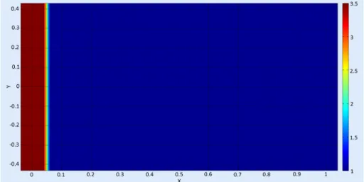
Figure 4.3: Fluid velocity in x direction, at the time 0.14s

Chapter 4. Moving Normal Shockwave 20

Figure 4.5: Fluid temperature, at the time 0.14s

Chapter 4. Moving Normal Shockwave 21

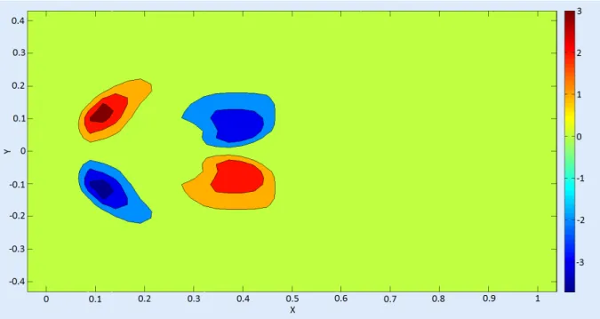
Figure 4.7: Fluid velocity in y direction, at the time 0.14s

Chapter 4. Moving Normal Shockwave 22

4.2.1 Carrier Phase

The flow behind the Shockwave is supersonic and has the same Mach number as the

shockwave while the upstream flow is at rest. Across the normal shock, the velocity

de-creases instantaneously to subsonic values, while the pressure, density and temperature

increase. As it is seen; by the moment the problem is analyzed, the shock is at x= 0.5

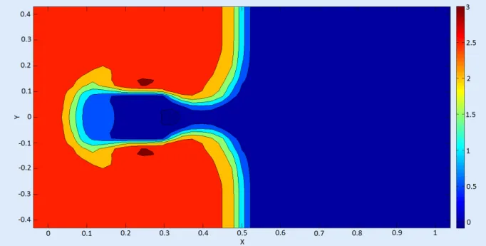
As the shock moves downstream and interacts with the cloud of particles, a bow shock

forms upstream of the cloud. This bow shock is called the induced shock to

differen-ciate it from the initial shock. The flow deccelerates across the induced shock, causing

a decrease in the kinetic energy of the carrier phase, (figure 4.3). Because no energy is

generated in the system, an increase in the internal and static energy of the flow

com-pensates for the decrease in kinetic energy as shown in figures 4.4 and 4.5. Following

the ideal gas law, the increased static energy results in an increase of the fluid density,

figure4.6.

After the induced schock, the flow interacts with the particles causing a gradual decrease

in the velocity, pressure and temperature. The decreased velocity, pressure and

temper-ature occur because of the energy and momentum transfer from the fluid to the particle

phase, while the increased density is due to the slowing of the fluid. The particles are

initiallized with zero velocity and in energy equilibrium with the Carrier Phase.

Figure 4.7 shows the velocity in y and in Figure 4.8 is shown the streamlines through

the particle cloud.

Chapter 4. Moving Normal Shockwave 23

Figure 4.10: Particle velocity in x direction, at the time 0.14s

Chapter 4. Moving Normal Shockwave 24

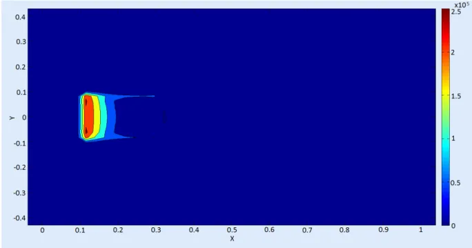
Figure 4.12: Particle temperature, at the time 0.14s

4.2.2 Disperse Phase

When the flow passes through the particle cloud, this experiments a decrease in the

kinetic, static and internal energy. The particles initially at the leading edge start

ac-celerating and overtaking the particles initially at the rear of the cloud. At later times,

more particles are accelerated due to the flow or pushed by other particles, hence the

cloud moves forward.

In figure 4.12, particle temperature is shown. The particles in the leading edge

experi-ment a larger increase of temperature because the temperature of the fluid in this area

is higher. The particle velocity in y presents a similar behaviour owing to the coupling

and momentum transfer between phases. Particles in the leading edge of the cloud are

pushed out of the cloud so these particles wil be spread away, while particles in the

trailing edge of the cloud are pushed into the cloud. This will mean that the cloud of

particles will be narrower and longer in the trailing edge but shorter and wider in the

Chapter 5

Conclusions and Future Work

A 2D Eulerian Eulerian model is presented to compute a two-way coupled particle laden

flow in a compressible fluid. The EE model couples the inviscid Euler equations with a

new set of Eulerian equations developed for the particle phase, derived with a filtered

Liouville equation that governs the particle density function. Second moments of the

particle phase result in a non-linear system of equatios while third moments are simplified

by asumming third order correlations are neglegible.

To linearize the problem, a Roe averaging scheme is used in the carrier phase and simple

averaging is used in the disperse phase. The model is discretized using a uniform grid and

fluxes are computed with a high order Weight Esentially Non-Oscillatory conservative

finite difference scheme, also known as high order WENO scheme. WENO methods have

high accuracy in smooth areas while providing good resolution around discontinuities as

well as the neccessary dissipation for shock capturing. In order to assure the stability

and convergence of the method, a CFL condition is used to modulate the time step.

Finally, time is updated with a RK3 scheme.

The interaction of a right-running normal shock and an initially stationary and in energy

equilibrium rectangular cloud of particles, is analyzed. Fluid is supersonic upstream and

subsonic downstream. The only mechanism that a supersonic flow has to adapt to an

obstacle like the cloud of particles is, is by a bow shock, also called induced shock. This

shock makes the velocity decrease to subsonic values and the pressure and termperature

increase. Following the ideal gas law, result in an increase of the density.

As the shock runs through the cloud of particles, fluid phase transfer energy and

mo-mentum to the particle phase, increasing the temperature of the particles at the leading

edge of the cloud while this particles start to accelerate downstream. The cloud is an

obstacle for the flow so the streamlines surround the cloud and this generates in the flow

Chapter 5. Conclusions and Future Work 26

a velocity in y. This velocity is also transferred to the particles making the cloud not

only move down stream but also change its initially rectangular shape.

Future lines would focus on comparing different ways to solve the problem since the EE

approach using a different scheme such us Godunov based schemes or high order upwind

schemes. Other future efforts could focus on compared the results between the EE and

Bibliography

[1] Truong, Q. Eulerian-Eulerian Model of 2D Normal Shock wave through a particle

cloud. Master’s thesis. San Diego State University, 2012.

[2] Shotorban B., Jacobs, G.B., Ortiz, O., Truong Q. An Eulerian model for particles

nonsiotermally carried by a compressible fluid. International Journal of Heat and Mass

Transfer, 65:845-854, 2013.

[3] Jacobs, G.B., Don, W.S. A High Order WENO-Z Finite Difference Based

Particle-Source-in-Cell Method for Computation of Particle-Laden Flows with Shocks, J. Comp.

Phys., 228 (5), 2009.

[4] Shu, C.W. High Order Weighted Essentially Nonoscillatory Scheme for Convection

Dominated Problems. Society for industrial and Applied Mathematics. 51(1), 82-126,

2009.

[5] Ortiz, O. Eulerian-Eulerian Model of 1D Compressible Particle-Laden Flow: Running

Shock Impingning on a Cloud of Particles. Master’s thesis. San Diego State University,

2011.