1
Estimation of PM10-bound As, Cd, Ni and Pb levels by means of statistical modelling: PLSR and ANN1
approaches
2
3
Authors:
Germán Santos*, Ignacio Fernández-Olmo, Ángel Irabien
4
5
Universidad de Cantabria, Dep. Ingenierías Química y Biomolecular, Avda. Los Castros s/n, 39005
6
Santander (Cantabria), Spain
7
8
*Corresponding author:9
Tel.:+34942201579; fax: +3494220159110
E-mail address: [email protected]
11
Manuscript validated
Click here to download Manuscript: Santos et al_manuscript_revised_validated.docx Click here to view linked References
2
1. Introduction12
13
Mathematical modelling for air quality assessment purposes has become increasingly important in recent
14
years. These models consist of a set of analytical/numerical algorithms that describe the physical and
15
chemical aspects of a problem and can be divided into two main groups: (i) deterministic models based on
16
fundamental mathematical descriptions of atmospheric processes, where emissions (causes) generate air
17
pollution (effects); (ii) statistical (empirical) models based on semiempirical statistical relations between
18
available data of input variables that are believed to be representative of the process behaviour and
19
measurements of the target parameters/properties of the system output. Moreover, the European Union Air
20
Quality Framework Directive establishes that in all zones and agglomerations where the level of pollutants
21
is below the lower assessment threshold (LAT), which is expressed as a percentage of the corresponding
22
target/limit value, modelling techniques or objective estimation techniques (or both) shall be sufficient for
23
the assessment of the ambient air quality (European Council Directive 2008/50/EC). Both statistical and
24
deterministic methods are currently used in regulatory air pollution forecasting by environmental
25
authorities.
26
27
Although deterministic models have some advantages over statistical models, such as a full-coverage 3D
28
domain, in some particular situations they may have some drawbacks in terms of accuracy and input data
29
uncertainty. According to Hanna (1989), generally, a larger number of input parameters corresponds to a
30
lower model uncertainty and smaller prediction errors, but unfortunately, by extending the number of input
31
parameters, the error and uncertainty attached to the input data also increase. Therefore, complex
32
deterministic models work well when their extensive input data requirements are satisfied, which rarely
33
occurs with some pollutants, such as As, Ni, Cd and Pb. This is due to the fact that the presence of these
34
pollutants in the atmosphere normally originates in a variety of pollution sources, not exclusively bound to
35
specific industrial activities at a certain location. As a consequence, the emission rates of these pollutants
36
from all the point or area sources are difficult to estimate. A solution to address this problem consists in
37
performing a spatial disaggregation of emission inventories (Maes et al. 2009). Notwithstanding, there is
38
an underlying uncertainty associated with the method of disaggregation together with the inherent
39
uncertainty of the emission inventories themselves. For that reason, for pollutants like the ones under study
40
in this work, the performance of complex models is often equal to that of simpler methodologies. This fact
41
3
highlights the interest of statistical models (e.g., linear regression techniques and non-linear modelling42
techniques) to estimate the ambient air concentration of atmospheric pollutants even though a wide range
43
of deterministic models, as reviewed by El-Harbawi (2013), have been already developed and studied in
44
the literature. Nevertheless, techniques such as partial least squares regression (PLSR), which presents
45
advantages over other statistical linear regression techniques because it combines features from factor
46
analysis statistical methods, such as principal component analysis (PCA) and linear regression techniques,
47
as multiple linear regression (MLR), may potentially lead to more accurate estimations than those provided
48
by MLR or principal component regression (PCR). Furthermore, according to Wold et al. (2001), although
49
regression techniques such as MLR works reasonably well with problems involving fairly few uncorrelated
50
independent variables, PLSR is preferable when analysing more intricate problems because it is able to
51
manage simultaneously numerous and collinear predictor variables and responses. Despite the fact that it
52
has been widely applied in other disciplines, chemometrics in particular, and used in some works related to
53
atmospheric pollution (Ogulei et al. 2006; Wingfors et al. 2001), there are few studies on the application of
54
PLSR to predict atmospheric pollutant concentrations. Pires et al. (2008) tested the ability of different linear
55
models, including PLSR, to predict daily mean concentrations of particles with an aerodynamic diameter
56
of less than 10 µm (PM10) in Oporto (Portugal). It was obtained that even though every model fitted the
57
data similarly well, PLSR shows higher generalization ability than other linear techniques. Polat and
58
Durduran (2012) used regression models such as least squares regression (LSR), PLSR and MLR to predict
59
daily particulate matter concentration values in the city of Konya (Turkey). PLSR performance, slightly
60
better than those of the other regression models, was remarkably improved by considering data
pre-61
processing methods such as output-dependent data scaling (ODDS). Singh et al. (2012) compared PLSR
62
with non-linear modelling approaches to predict respirable suspended particulate matter (RSPM), SO2 and
63
NO2 in Lucknow city (India). Both linear and non-linear approaches provided adequate estimations,
64
especially for the RSPM, with values of correlation coefficient up to 0.9. Nonetheless, non-linear models
65
performed relatively better than the linear PLSR models.
66
67
With respect to non-linear modelling approaches, artificial neural networks (ANNs) have been suggested
68
as fair alternatives to statistical linear regression methods because they usually provide equal or superior
69
results, especially when there is non-linear behaviour involved in the problem under analysis, i.e., cases in
70
the atmospheric sciences (Gardner and Dorling 1998). For this reason, ANNs are particularly expected to
71
4
produce good predictive results when modelling PM mass concentrations compared with common gaseous72
pollutants based on their ability to capture the highly non-linear character of the complex processes that
73
control the formation, transportation and removal of aerosols in the atmosphere (Grivas and Chaloulakou
74
2006). Furthermore, ANNs have been extensively applied in the past in the atmospheric literature with
75
successful results regarding forecasting major gaseous air pollutant concentrations, such as nitrogen oxides
76
(Gardner and Dorling 1999; Kolehmainen et al. 2001; Lu et al. 2003), sulphur dioxide (Chelani et al.
77
2002a), and (commonly) ozone (Abdul-Wahab and Al-Alawi 2002; Chaloulakou et al. 2003; Comrie 1997;
78
Inal 2010; Sousa et al. 2007; Wang et al. 2003; Yi and Prybutok 1996). Moreover, a number of studies have
79
been conducted using ANN approaches to forecast airborne PM mass concentrations (Caselli et al. 2009;
80
Chelani 2005; Grivas and Chaloulakou 2006; Hoi et al. 2009; Kim et al. 2009; Papanastasiou et al. 2007;
81
Paschalidou et al. 2011; Perez and Reyes 2002; Perez and Reyes 2006; Pérez et al. 2000; Voukantsis et al.
82
2011), predict PM mass concentrations, and predict other gaseous pollutant concentrations (Brunelli et al.
83
2007; Cai et al. 2009; Hrust et al. 2009; Jiang et al. 2004; Kukkonen et al. 2003; Kurt et al. 2008; Lu et al.
84
2004; Lu et al. 2003; Niska et al. 2005; Turias et al. 2008). Nevertheless, regarding the PM composition
85
and estimation of PM constituents, few studies have been conducted. In particular, with respect to the metal
86
content in PM, Chelani et al. (2002b) used ANNs to predict ambient PM10 and metals, such as Cd, Cr, Fe,
87
Ni, Pb and Zn, in the air of Jaipur, India, in 1999. It was observed that the ANN models were able to predict
88
all the pollutant concentrations with low values of root means square error (RMSE). Nonetheless, more
89
studies related to atmospheric metal concentration estimations by means of ANNs have been conducted,
90
such as the study performed by Li et al. (2009) in which statistical models based on back-propagation ANNs
91
and MLR are applied to reconstruct occupational manganese exposure. Apart from ANNs, some research
92
has been conducted to model metal concentrations in ambient air using other statistical approaches.
93
Hernández et al. (1992) applied state-space modelling, Box-Jenkins modelling and time series
94
autoregressive integrated moving average (ARIMA) models to estimate the daily concentrations of
air-95
particulate Fe and Pb in Madrid (Spain). Predictions of daily Fe were better than those of Pb. No difference
96
being found between State-space and Box-Jenkins models, their outcomes were better than those of
97
ARIMA models in terms of root mean squared error (RMSE), correlation coefficient and efficiency.
98
Chelani et al. (2001) used a state-space model coupled with Kalman filter and an autoregressive model with
99
external input (ARX model) to forecast Pb, Fe and Zn along with RSPM in Delhi (India). The state space
100
model performed better than the ARX model. On the other hand, Vicente et al. (2012) developed predictive
101
5
models based on multiple regression analysis together with time series (ARIMA) models to predict the102
concentration of total suspended particles (TSP), PM10, As, Cd, Ni and Pb in the ambient air of Castellón
103
(Spain). Furthermore, in a previous study conducted by Arruti et al. (2011), estimations of As, Cd, Ni and
104
Pb levels in Cantabria (Spain) by means of statistical MLR and PCR models have been conducted. It is
105
concluded that both represent valid approaches as objective estimation techniques.
106
107
This paper is focused on the development of PLSR and ANN statistical models to estimate the levels of As,
108
Cd, Ni and Pb in the ambient air of two urban areas: Castro Urdiales and Reinosa in the Cantabria region
109
(northern Spain). These models are evaluated according to the uncertainty requirements established by the
110
EU for objective estimation techniques as well as for their ability to estimate the mean concentration.
111
Additionally, an external validation of the models developed is performed.
112
113
2. Materials and methods
114
115
2.1. Statistical model fundamentals
116
117
2.1.1. Partial least squares regression (PLSR)
118
119
Partial least squares regression is a multivariate calibration technique whose aim is to investigate the
120
relationship between a set of dependent variables or responses and a set of independent variables known as
121
predictors. Firstly, in a similar manner to PCA, PLSR performs a decomposition of the original predictor
122
variables (X-matrix, which consists of environmental observations in this study) by projecting them to a
123
new space and extracts a set of orthogonal factors, called latent variables, which have the best predictive
124
ability. Simultaneously, a decomposition of the response variables (Y-matrix, composed of metal level
125
observations) is also performed. This decomposition step is made in a manner that the projections (scores)
126
of X have maximum covariance with the projections of Y. This procedure is followed by a regression stage,
127
where PLSR (just as MLR) creates a linear combination of the predictor variables in order to predict Y
128
(Abdi 2010).
129
6
In this work, cross-validation techniques were used to select the more suitable number of significant131
components. PLS Toolbox (Eigenvector Research, Inc.) for MATLAB was used in the present study to
132
develop the PLSR models.
133
134
2.1.2. Artificial neural networks (ANNs)
135
136
Artificial neural networks are computational systems inspired by the biological central nervous system.
137
They consist of a number of simple process elements, commonly referred to as artificial neurons, which are
138
logically arranged into layers, highly interconnected, and interact with each other via weighted connections.
139
Through a supervised training process, in which they are successively presented with a series of input and
140
associated output data, ANNs are capable to learn to model highly non-linear relationships and, as a result,
141
to accurately generalise when previously unseen data are presented afterwards. The reader is referred the
142
handbooks of Bishop (1995) and Hassoun (1995) for a comprehensive description of the ANN technique.
143
144
Plenty of neural network architectures exist. In this work, based on the different ANN approaches found in
145
the air quality related literature, a multilayer perceptron (MLP) neural network architecture was selected;
146
details of the architecture are provided in Gardner and Dorling (1998).
147
148
Because the ratio of input variables/number of samples is relatively high in this work due to the number of
149
samples that were collected by the Regional Environmental Ministry, applying a dimension reduction
150
technique prior to the ANN models was expected to produce an improvement in the estimations as reported
151
in some studies (Lu et al. 2003; Sousa et al. 2007). Therefore, an alternative approach in which the PCA is
152
performed before the development of the ANN models (hereafter known as PCA-ANNs) is considered.
153
154
The ANN models in this study were developed using the Neural Network Toolbox for MATLAB
155
(MathWorks, Inc.).156
157
2.2. Study area158
159
7
Two urban areas in the Cantabria region (northern Spain) whose air quality may be influenced by the160
presence of metallurgical and other industrial activities in their vicinity were selected: Castro Urdiales and
161
Reinosa (Fig. 1). The former area is a coastal urban site at the NE zone of Cantabria which has 32258
162
(2010) inhabitants and encompasses an area of approximately 97 km2. Pollution in this area has a marked
163
anthropogenic origin which is caused by traffic, not in vain Castro Urdiales is surrounded by the main
164
national highway in the northern part of Spain. Pollution also proceeds from industrial activities, such as
165
chemical and metallurgical plants and an oil refinery, located 10-30 km SE (near the city of Bilbao). The
166
monitoring station is located at 43º22’53”N, 3º13’22” W and 20 m above sea level, in the core of the urban
167
area. In contrast, Reinosa, covering nearly 4 km2 with approximately 10277 inhabitants (2010), is located
168
inland, at about 50 km off the shore, in the southern part of the region. The sampling station is located at
169
43º00’01”N, 4º08’13”W and 850 m above sea level. It is in close proximity to a steel manufacturing plant
170
and also to a national highway, main exit route from Cantabria, which establishes connection with the
171
central Iberian Peninsula.
172
173
2.3. Input dataset
174
175
The dataset used in this study is divided into response variables and predictor variables. The former data
176
consist of As, Cd, Ni and Pb concentrations (ng m-3) in airborne PM
10 for the period from 2008 to 2010 at
177
the two study sites. The PM10 sampling was performed by the Cantabrian Regional Environmental Ministry
178
according to the reference method for the determination of the PM10 fraction of suspended particulate matter
179
detailed in standard UNE-EN 12341:1999. 48h averaged samples of PM10 were taken once every two weeks
180
for the period from 2008 to 2009 and 24h averaged samples of PM10 were collected for 2010 with a weekly
181
sampling frequency. The content of a number of metals and metalloids in the PM10 samples was determined
182
by our research group based on the standard method for the measurement of Pb, Cd, As and Ni in the PM10
183
fraction of the suspended particulate matter described in standard UNE-EN 14902:2006. According to this,
184
after gravimetric determination of the particle concentration levels, the PM10 filters were treated with
185
microwave-assisted acid digestion to extract the analytes into an aqueous solution prior to the analytical
186
determination of their concentration by inductively coupled plasma mass spectroscopy (ICP-MS). Further
187
details of this analytical method can be found in Arruti et al. (2010).
188
8
As a consequence of the high cost associated with the analytical determination of the content of this sort of190
pollutants in particulate matter, a considerably low number of samples was selected for the analysis.
191
However, this number was sufficient to guarantee the minimum time coverage (14%) for indicative
192
measurements as European Council Directive 2004/107/EC requires.
193
194
The predictor variables are qualitative or nominal variables (Table 1) that take into account seasonal effects,
195
Saharan dust intrusion and weekend effects or quantitative or continuous variables, namely, meteorological
196
data and major atmospheric pollutant concentration, which are detailed in Table 2. With respect to the
197
nominal variables, the information regarding the occurrence of Saharan dust intrusion events has been
198
obtained from annual reports on African dust episodes over Spain (MAGRAMA 2015), which are
199
developed by the Spanish National Research Council (CSIC) in collaboration with the Spanish Ministry of
200
Agriculture, Food and Environment. In contrast, the continuous variables are measured automatically in
201
real time (maximum time resolution of fifteen minutes) at the monitoring stations of the Cantabrian
202
Regional Air Quality Monitoring Network located in the study sites and are available at the Regional
203
Environment Ministry website. Average values of continuous variables were calculated according to the
204
corresponding duration of the PM10 sampling periods (48 hours for 2008-2009 samples and 24 hours for
205
2010 samples). Moreover, as regards to PM10 concentration, it has been included as input variable in the
206
form of natural logarithm because of this transformation being reported to improve the performance of
207
regression models (Arruti et al. 2011).
208
209
Prior to model development it is always rather convenient to take account of the application of a data
pre-210
processing method, especially if there is lack of knowledge regarding the relative importance of the
211
variables. In this study, the following data pre-treatment procedure was applied:
212
213
1. Dependent variable normalisation by the respective LAT in order to minimise scale effects.
214
2. Input variable auto-scaling, subtracting the mean and dividing by the standard deviation, in an attempt
215
to make each variable a priori equally important.
216
3. Multivariate outlier identification and removal method based on Mahalanobis distance. It is a
well-217
known classical approach that computes the Mahalanobis distance (MD) of each observation as an
218
indicative measure of the distance of each data point from the centre of the multivariate data cloud. By
219
9
convention, this method identifies as outliers those observations with a large MD (exceeding the 99%220
quantile of a chi-square distribution).
221
222
Apart from the data pre-processing treatment, over-fitting is another decisive matter that must be taken into
223
consideration beforehand so that it could be prevented. This term refers to the circumstance that occurs
224
when a model fit the data in such a manner that not only captures the underlying trend in the data but also
225
the unexplained variation or statistical noise and therefore it is unable to generalize properly - that is, to
226
correctly perform when new observations are presented. In order to overcome this phenomenon it is highly
227
recommended the consideration of an additional verification or cross-validation data subset, besides the
228
training or fitting dataset, to check the models performance during the model development stage (usually
229
known as calibration or fitting for PLSR and training for ANNs). Additionally, if the generalisation ability
230
of a model is to be tested, a subset of samples has to be kept in reserve to perform an external validation
231
with previously unused observations once the models have been developed. For that reason, the complete
232
dataset was divided into three different subsets: 60% for training/fitting, 20% for verification and 20% for
233
external validation. Data partition of the available data, often randomly conducted, was carried out in this
234
work by means of the Kennard-Stone algorithm (Kennard and Stone 1969) with the purpose that the
235
resulting subsets are statistically representative. This data division method, originally developed for design
236
of experiments, has been traditionally applied to select calibration samples extracting subsets, as much
237
diverse as possible, from a large set of candidate samples based on the Euclidean distance, which is
238
employed as a measure of similarity between samples (the lower the Euclidean distance, the higher the
239
similarity). Initially, the pair of samples with the largest Euclidean distance are selected. Subsequently, by
240
means of an iterative process that concludes when the number of required objects is reached, more samples
241
are selected, maximizing the minimal Euclidean distances between those already selected and the remaining
242
samples.243
244
2.4. Model evaluation245
246
The main criteria employed in this work to determine whether a model is suitable for air quality assessment
247
purposes is principally based on two aspects: (i) the fulfilment of the European Union uncertainty
248
requirements for objective estimation techniques, which are shown in Table 3 and (ii) the accuracy of
249
10
estimated mean values. Additionally, a number of statistical parameters has been considered to evaluate the250
modelling performance and are also shown in Table 3.
251
252
3. Results and discussion
253
254
3.1. As, Cd, Ni and Pb levels in Castro Urdiales and Reinosa
255
256
Fig. 2 summarises the levels of As, Cd, Ni and Pb in PM10 at Castro Urdiales and Reinosa for the period
257
from 2008 to 2010. According to the European Council Directive 2008/50/EC, because these levels did not
258
exceed their lower assessment threshold and did not present significant variations throughout the period of
259
study, modelling and objective estimation techniques are permitted as an alternative method to experimental
260
measurements for air quality assessment.
261
262
3.2. Statistical estimation models for Castro Urdiales
263
264
Table 4 shows the results relating to the best-developed models at the Castro Urdiales site for the four
265
pollutants under study using the three approaches: PLSR, ANNs and PCA coupled with ANNs. The results
266
obtained for both the training and the external validation subsets are presented.
267
268
Limit/target values for As, Cd, Ni and Pb in ambient air in the European regulations are given in annual
269
mean concentration values. Therefore, attention should be paid to the estimated mean concentrations in the
270
study period. The normalised mean concentrations are presented in Table 4. The accuracy in the estimation
271
of the mean concentration is evaluated by means of the fractional bias (FB) index. In this respect, the
272
estimations are more accurate for the training step. At this step, PLSR provides a FB index lower than those
273
obtained for ANNs and PCA-ANNs because the mean metal concentration estimated by the PLSR models
274
are equal —up to two significant figures— to the corresponding observed values and that, according to the
275
corresponding equation (Table 3), yields lower FB index values. However, the differences between
276
estimated and observed mean concentrations using the three considered techniques are not remarkably
277
significant. As for external validation, the precision is inferior to that of the training phase.
278
11
In a more illustrative way, Fig. 3 represents the mean metal concentration estimation expressed as a280
percentage of the corresponding limit/target value. The vertical axis is presented in logarithmic scale. The
281
green area represents the zone below the LAT, the yellow area represents the zone between the UAT and
282
the LAT, and the red area is the zone between the limit/target value and the UAT. Fig. 3 shows that, even
283
though there are some differences between the estimated and the observed mean levels, they are similar.
284
Moreover, because the observed metal(loid) levels are within the green area, well below the LAT, even
285
higher discrepancy could be allowed. Therefore, the developed models provide satisfactory mean
286
concentration estimations.
287
288
It is necessary to validate objective estimation techniques in the context of the EU Directives in terms of
289
uncertainty. In this sense, according to Arruti et al. (2011), two indices have been considered: on the one
290
hand, the RME, which is defined as the largest concentration difference of all percentile differences
291
normalized by the respective observed value (Fleming and Stern 2007); on the other hand, the RDE, which
292
evaluates the accuracy in the estimation of the observation closest to the limit/target value (Denby 2009).
293
As observed in Table 4, the values of these indices for the four pollutants in question for the training and
294
the external validation are well below 100%, which is the maximum permissible uncertainty limit for using
295
objective estimation techniques as air quality assessment tools according to the European Council Directive
296
2008/50/EC. For As, Ni and Cd, ANNs provide higher RME values than PLSR and PCA-ANN. In the
297
majority of cases, except for the As and Cd ANN models, the RME values are below 50%, which is the
298
uncertainty requirement for modelling techniques. In all cases, the RDE values are below 10%. However,
299
these indices have some limitations: it has been discussed that RME is sensitive to the presence of outliers
300
resulting in an increase of the uncertainty values (Fleming and Stern 2007); RDE only evaluates the
301
uncertainty of just one sample, the closest to the limit/target value.
302
303
From a scientific point of view, apart from a precise estimation of mean values to comply with the policy
304
framework, a model should be able to correctly describe the temporal variations of dependent variables.
305
For this purpose, a set of statistics has been used in this work. In the first place, the correlation coefficient
306
is employed to measure the goodness of fit between the observed and the estimated values. The results
307
show that PLSR correlation coefficients, which are within the range of 0.6-0.7, are less variable than those
308
of ANNs and PCA-ANNs: whereas the highest correlation coefficient, an r value of 0.82, is found when
309
12
using ANNs for Pb training, the correlation coefficients for As and Cd ANN models are significantly low310
and therefore unacceptable. This could be explained because in the area of study As and Cd tend to be in
311
lower concentration than Ni and Pb and consequently in the period of study a number of samples have
312
levels of As and Cd below their detection limits. As a result, models are trained to produce the same output
313
from different inputs, a detrimental contradiction that may negatively affect the estimation of the rest of the
314
samples. Moreover, as expected, the r values for external validation are often lower than those for training.
315
Nonetheless, the PCA-ANN external validation correlation coefficients are systematically below 0.5.
316
317
In addition to the correlation coefficient, the precision of the individual sample concentration estimation is
318
quantified by the RMSE, the NMSE and the FV, (see equations in Table 3). The RMSE values, which
319
provide information regarding the differences between the observed and estimated concentrations, are
320
shown in Table 4. However, to compare these differences for different approaches and pollutants, a
321
normalised version of this parameter (NMSE) is more preferable because it does not take into account the
322
range of the independent variable. In general, the three considered approaches provide low values of NMSE
323
in the order of 10-1.
324
325
With respect to the FV index, positive values can be observed in Table 4; this indicates that the estimated
326
variance is lower than the observed variance. Therefore, estimated values are less dispersed than observed
327
values, which tend to be more distanced from the mean value. This fact, together with a positive FB
328
corresponding to a slight mean value underestimation, indicates that there are some shortcomings in the
329
model capacity to perfectly describe all the concentration variations, especially regarding peak values.
330
Nevertheless, despite no substantial differences being found when comparing PLSR and ANNs, in general
331
both models are able to capture the underlying trend and provide temporal variations with similar shape to
332
that of the observed values as depicted in Fig. 4 for Pb and Ni in the training stage.
333
334
Based on the results obtained, there is no improvement associated with considering a dimension reduction
335
technique such as PCA before the development of the ANNs. This could be accounted for the fact that most
336
ANNs suffer less from the curse of dimensionality than some other techniques, as they can concentrate on
337
a lower dimensional section of the high-dimensional space, which may be done, for instance, by
338
disregarding completely an input, setting the corresponding weights to zero. Hence, for this specific
339
13
application dimensionality reduction has been proven not to be effective because removing input variables340
from the analysis entails a loss on the predictive ability of the model.
341
342
Furthermore, because these models are devised to be used when the pollutant levels are sufficiently lower
343
at a certain location, in principle the moderated inaccuracy to estimate peak values should not represent an
344
unacceptable drawback to acknowledge these models as proper approaches complying with regulatory
345
requirements: the uncertainty values obtained with the developed models and the accuracy in the estimation
346
of the mean values would be favourable enough from a regulatory perspective. Nonetheless, some
347
refinement is possible because, as mentioned, there are some difficulties in estimating the highest observed
348
concentrations, which are underestimated. In this regard, further work involving new additional input
349
variables and the enlargement of the database with additional samples from different periods of time would
350
be recommendable.
351
352
3.3. Statistical estimation models for Reinosa
353
354
Analogously to the results at the Castro Urdiales site, the statistical parameters corresponding to the
best-355
developed models at the Reinosa site are presented in Table 5.
356
357
Regarding the uncertainty indices, it is observed that, as in Castro Urdiales, the RME and RDE values at
358
the Reinosa site are below 100% for the estimations obtained with the three different models developed for
359
the four pollutants. Hence, the quality objectives for ambient air quality assessment by means of objective
360
estimation techniques are met. However, there is a general increase in the obtained RDE values, especially
361
for As and Ni, which are significantly greater than those obtained at the Castro Urdiales site.
362
363
In relation to the mean values, again, PLSR provides the lowest FB training values, but the FB external
364
validation values are greater than the training values. Although there are still evident differences between
365
the observed and estimated mean concentrations, 90% of the estimations do not differ by more than 50%.
366
Therefore, as shown in Fig. 5, the three developed models provide satisfactory estimations. Nonetheless, a
367
substantial increase in FB values is found in Reinosa compared with Castro Urdiales.
368
14
Results at the Reinosa site present more variability between the training and external validation correlation370
coefficient values for each pollutant than the results at the Castro Urdiales site, which may be partially
371
accounted for the higher inherent variance of metal levels in Reinosa compared to those obtained in Castro
372
Urdiales. However, the ANN correlation coefficient values are generally equal or superior to those of PLSR
373
and PCA-ANNs. As for the errors in the individual sample concentration estimations, the NMSE values for
374
Reinosa and Castro Urdiales are within the same range. Nevertheless, the FV values are slightly greater in
375
Reinosa than in Castro Urdiales but still lower than 1.0, which represents 50% of the observed variance.
376
377
Results prove that these models provide an acceptable performance in varied areas of a region, even when
378
there is a complex pollution framework with diverse emission sources, as is the case of Castro Urdiales.
379
Nevertheless, because the models were trained on data for particular sites and having been demonstrated
380
that the precision in the estimation is dependent on the specific location, these models can therefore only
381
be used with confidence at those sites. This dependence is especially pronounced in the ANN models, which
382
produced a higher variability in the results than the PLSR or PCA-ANN models. This may be influenced
383
by the fact that a limited number of samples are used for developing the models due to the unavailability
384
of additional observations stemming from their costliness and time consumption. Thus, it could be inferred
385
that for small datasets, linear regression techniques can work as well as non-linear modelling approaches
386
in terms of the estimation of metal(loid) levels in ambient air.
387
388
4. Conclusions
389
390
Statistical models are developed as objective estimation techniques to estimate the As, Cd, Ni and Pb in
391
ambient air at a local scale in two urban areas in the Cantabria region (northern Spain): Castro Urdiales and
392
Reinosa. These models were built based on linear regression techniques, partial least squares regression
393
(PLSR), and the non-linear modelling technique of artificial neural networks (ANNs). Additionally, an
394
alternative approach is considered that performs principal component analysis (PCA) prior to the ANN
395
analysis (PCA-ANNs). Furthermore, these models were externally validated using previously unseen data.
396
397
The models are evaluated by means of a number of statistical parameters, including uncertainty indices, to
398
determine if they comply with the EU quality requirements for objective estimation techniques.
399
15
Additionally, the model performance in estimating the individual sample concentrations is evaluated by400
means of a number of statistical parameters, including a correlation coefficient, RMSE, NMSE and FV.
401
402
Based on the results obtained, PLSR and ANN techniques are acceptable alternatives to estimate the mean
403
concentration of As, Cd, Ni and Pb for the period of study in the two considered sites while fulfilling the
404
uncertainty requirements for objective estimation techniques established in the EU Directives.
405
Consequently, PLSR and ANN-based statistical models represent a proper alternative to experimental
406
measurements for air quality assessment purposes in the area of study. However, ANNs have not
407
demonstrated to offer a clear superior performance over the linear regression technique, what may be
408
attributed to the modest size of the available database. Furthermore, the three considered approaches had
409
some difficulties providing accurate estimations of the levels of individual samples, particularly for the
410
external validation subset. Moreover, the application of PCA before the ANN model development did not
411
yield an improvement of the models.
412
413
Acknowledgements
414
415
The authors gratefully acknowledge the financial support from the Spanish Ministry of Economy and
416
Competitiveness through the Project CMT2010-16068. The authors also thank the Regional Environment
417
Ministry of the Cantabria Government for providing the PM10 samples at the Castro Urdiales and Reinosa
418
sites.419
420
References421
422
Abdi, H. (2010). Partial least squares regression and projection on latent structure regression (PLS
423
Regression). Wiley Interdisciplinary Reviews: Computational Statistics, 2(1), 97-106.
424
425
Abdul-Wahab, S. A., & Al-Alawi, S. M. (2002). Assessment and prediction of tropospheric ozone
426
concentration levels using artificial neural networks. Environmental Modelling and Software, 17(3),
219-427
228.
428
16
Arruti, A., Fernández-Olmo, I., & Irabien, A. (2010). Evaluation of the contribution of local sources to430
trace metals levels in urban PM2.5 and PM10 in the Cantabria Region (Northern Spain). Journal of
431
Environmental Monitoring, 12, 1451-1458.
432
433
Arruti, A., Fernández-Olmo, I., & Irabien, A. (2011). Assessment of regional metal levels in ambient air
434
by statistical regression models. Journal of Environmental Monitoring, 13(7), 1991-2000.
435
436
Bishop, C. M. (1995). Neural Networks for Pattern Recognition and Machine Learning. Oxford: Clarendon
437
Press.
438
439
Brunelli, U., Piazza, V., Pignato, L., Sorbello, F., & Vitabile, S. (2007). Two-days ahead prediction of daily
440
maximum concentrations of SO2, O3, PM10, NO2, CO in the urban area of Palermo, Italy. Atmospheric
441
Environment, 41(14), 2967-2995.
442
443
Cai, M., Yin, Y., & Xie, M. (2009). Prediction of hourly air pollutant concentrations near urban arterials
444
using artificial neural network approach. Transportation Research Part D: Transport and Environment,
445
14(1), 32-41.
446
447
Caselli, M., Trizio, L., De Gennaro, G., & Ielpo, P. (2009). A simple feedforward neural network for the
448
PM10 forecasting: Comparison with a radial basis function network and a multivariate linear regression
449
model. Water, air, and soil pollution, 201(1-4), 365-377.
450
451
Chaloulakou, A., Saisana, M., & Spyrellis, N. (2003). Comparative assessment of neural networks and
452
regression models for forecasting summertime ozone in Athens. Science of the Total Environment,
313(1-453
3), 1-13.
454
455
Chelani, A. B., Gajghate, D. G., Tamhane, S. M., & Hasan, M. Z. (2001). Statistical modeling of ambient
456
air pollutants in Delhi. Water, air, and soil pollution, 132(3-4), 315-331.
457
17
Chelani, A. B., Chalapati Rao, C. V., Phadke, K. M., & Hasan, M. Z. (2002a). Prediction of sulphur dioxide459
concentration using artificial neural networks. Environmental Modelling and Software, 17(2), 161-168.
460
461
Chelani, A. B., Gajghate, D. G., & Hasan, M. Z. (2002b). Prediction of ambient PM10 and toxic metals
462
using artificial neural networks. Journal of the Air and Waste Management Association, 52(7), 805-810.
463
464
Chelani, A. B. (2005). Predicting chaotic time series of PM10 concentration using artificial neural network.
465
International Journal of Environmental Studies, 62(2), 181-191.
466
467
Comrie, A. C. (1997). Comparing neural networks and regression models for ozone forecasting. Journal of
468
the Air and Waste Management Association, 47(6), 653-663.
469
470
Denby, B. (2009). Guidance on the use of the models for the European Air Quality Directive. A Working
471
document of the Forum for Air Qualtiy Modelling in Europe, FAIRMODE. ETC/ACC Report.
472
473
El-Harbawi, M. (2013). Air quality modelling, simulation, and computational methods: A review.
474
Environmental Reviews, 21(3), 149-179.
475
476
Fleming, J., & Stern, R. (2007). Testing model accuracy measures according to the EU directives-examples
477
using the chemical transport model REM-CALGRID. Atmospheric Environment, 41, 9206-9216.
478
479
Gardner, M. W., & Dorling, S. R. (1998). Artificial neural networks (the multilayer perceptron) - a review
480
of applications in the atmospheric sciences. Atmospheric Environment, 32(14-15), 2627-2636.
481
482
Gardner, M. W., & Dorling, S. R. (1999). Neural network modelling and prediction of hourly NOx and NO2
483
concentrations in urban air in London. Atmospheric Environment, 33(5), 709-719.
484
485
Grivas, G., & Chaloulakou, A. (2006). Artificial neural network models for prediction of PM10 hourly
486
concentrations, in the Greater Area of Athens, Greece. Atmospheric Environment, 40(7), 1216-1229.
487
18
Hanna, S. R. (1989). Plume dispersion and concentration fluctuations in the atmosphere. In P.N.489
Cheremisinoff (Ed.), Encyclopedia of Environmental Control Technology, Vol. 2, Air Pollution Control.
490
Houston, Texas: Gulf Publishing Co.
491
492
Hassoun, M. H. (1995). Fundamentals of Artificial Neural Networks. London, England: MIT Press.
493
Hernández, E., Martín, F., & Valero, F. (1992). Statistical forecast models for daily air particulate iron and
494
lead concentrations for Madrid, Spain. Atmospheric Environment, 26B, 107-116.
495
496
Hoi, K. I., Yuen, K. V., & Mok, K. M. (2009). Prediction of daily averaged PM10 concentrations by
497
statistical time-varying model. Atmospheric Environment, 43(16), 2579-2581.
498
499
Hrust, L., Klaic, Z. B., Križan, J., Antonic, O., & Hercog, P. (2009). Neural network forecasting of air
500
pollutants hourly concentrations using optimised temporal averages of meteorological variables and
501
pollutant concentrations. Atmospheric Environment, 43(35), 5588-5596.
502
503
Inal, F. (2010). Artificial Neural Network Prediction of Tropospheric Ozone Concentrations in Istanbul,
504
Turkey. Clean - Soil, Air, Water, 38(10), 981.
505
506
Jiang, D., Zhang, Y., Hu, X., Zeng, Y., Tan, J., & Shao, D. (2004). Progress in developing an ANN model
507
for air pollution index forecast. Atmospheric Environment, 38(40 SPEC.ISS.), 7055-7064.
508
509
Kennard, R. W., & Stone, L. A. (1969). Computer aided design of experiments. Technometrics, 11(1),
137-510
148.
511
512
Kim, M., Kim, Y., Sung, S., & Yoo, C. (2009). Data-driven prediction model of indoor air quality by the
513
preprocessed recurrent neural networks. ICCAS-SICE 2009 - ICROS-SICE International Joint Conference
514
2009, Proceedings, 1688-1692.
515
516
Kolehmainen, M., Martikainen, H., & Ruuskanen, J. (2001). Neural networks and periodic components
517
used in air quality forecasting. Atmospheric Environment, 35(5), 815-825.
518
19
519
Kukkonen, J., Partanen, L., Karppinen, A., Ruuskanen, J., Junninen, H., Kolehmainen, M., Niska, H.,
520
Dorling, S., Chatterton, T., Foxall, R., & Cawley, G. (2003). Extensive evaluation of neural network models
521
for the prediction of NO2 and PM10 concentrations, compared with a deterministic modelling system and
522
measurements in central Helsinki. Atmospheric Environment, 37(32), 4539-4550.
523
524
Kurt, A., Gulbagci, B., Karaca, F., & Alagha, O. (2008). An online air pollution forecasting system using
525
neural networks. Environment international, 34(5), 592-598.
526
527
Li, Y., Luo, F., Jiang, Y., Lu, Y., Huang, J., & Zhang, Z. (2009). A prediction model of occupational
528
manganese exposure based on artificial neural network. Toxicology Mechanisms and Methods, 19(5),
337-529
345.
530
531
Lu, W. Z., Wang, W. J., Wang, X. K., Xu, Z. B., & Leung, A. Y. T. (2003). Using improved neural network
532
model to analyze RSP, NOX and NO2 levels in urban air in Mong Kok, Hong Kong. Environmental
533
monitoring and assessment, 87(3), 235-254.
534
535
Lu, W., Wang, W., Wang, X., Yan, S., & Lam, J. C. (2004). Potential assessment of a neural network model
536
with PCA/RBF approach for forecasting pollutant trends in Mong Kok urban air, Hong Kong.
537
Environmental research, 96(1), 79-87.
538
539
Maes, J., Vliegen, J., Van de Vel, K., Janssen, S., Deutsch, F., De Ridder, K., Mensink, C. (2009). Spatial
540
surrogates for the disaggregation of CORINAIR emission inventories. Atmospheric Environment, 43,
1246-541
1254.
542
543
Ministerio de Agricultura, Alimentación y Medio Ambiente (MAGRAMA), 2015. Histórico de informes
544
de episodios naturales.
http://www.magrama.gob.es/es/calidad-y-evaluacion-ambiental/temas/atmosfera-545
y-calidad-del-aire/calidad-del-aire/gestion/anuales.aspx
546
20
Niska, H., Rantamäki, M., Hiltunen, T., Karppinen, A., Kukkonen, J., Ruuskanen, J., & Kolehmainen, M.548
(2005). Evaluation of an integrated modelling system containing a multi-layer perceptron model and the
549
numerical weather prediction model HIRLAM for the forecasting of urban airborne pollutant
550
concentrations. Atmospheric Environment, 39(35), 6524-6536.
551
552
Ogulei, D., Hopke, P. K., Zhou, L., Patrick Pancras, J., Nair, N., & Ondov, J. M. (2006). Source
553
apportionment of Baltimore aerosol from combined size distribution and chemical composition data.
554
Atmospheric Environment, 40(SUPPL. 2), 396-410.
555
556
Papanastasiou, D. K., Melas, D., & Kioutsioukis, I. (2007). Development and assessment of neural network
557
and multiple regression models in order to predict PM10 levels in a medium-sized Mediterranean city.
558
Water, air, and soil pollution, 182(1-4), 325-334.
559
560
Paschalidou, A. K., Karakitsios, S., Kleanthous, S., & Kassomenos, P. A. (2011). Forecasting hourly PM10
561
concentration in Cyprus through artificial neural networks and multiple regression models: Implications to
562
local environmental management. Environmental Science and Pollution Research, 18(2), 316-327.
563
564
Pérez, P., Trier, A., & Reyes, J. (2000). Prediction of PM2.5 concentrations several hours in advance using
565
neural networks in Santiago, Chile. Atmospheric Environment, 34(8), 1189-1196.
566
567
Perez, P., & Reyes, J. (2002). Prediction of maximum of 24-h average of PM10 concentrations 30h in
568
advance in Santiago, Chile. Atmospheric Environment, 36(28), 4555-4561.
569
570
Perez, P., & Reyes, J. (2006). An integrated neural network model for PM10 forecasting. Atmospheric
571
Environment, 40(16), 2845-2851.
572
573
Pires, J. C. M., Martins, F. G., Sousa, S. I. V., Alvim-Ferraz, M. C. M., & Pereira, M. C. (2008). Prediction
574
of the daily mean PM10 concentrations using linear models. American Journal of Environmental Sciences,
575
4(5), 445-453.
576
21
Polat, K., & Durduran, S. S. (2012). Usage of output-dependent data scaling in modeling and prediction of578
air pollution daily concentration values (PM10) in the city of Konya. Neural Computing and Applications,
579
21(8), 2153-2162.
580
581
Singh, K. P., Gupta, S., Kumar, A., & Shukla, S. P. (2012). Linear and nonlinear modeling approaches for
582
urban air quality prediction. Science of the Total Environment, 426, 244-255.
583
584
Sousa, S. I. V., Martins, F. G., Alvim-Ferraz, M. C. M., & Pereira, M. C. (2007). Multiple linear regression
585
and artificial neural networks based on principal components to predict ozone concentrations.
586
Environmental Modelling and Software, 22(1), 97-103.
587
588
Turias, I. J., González, F. J., Martin, M. L., & Galindo, P. L. (2008). Prediction models of CO, SPM and
589
SO2 concentrations in the Campo de Gibraltar Region, Spain: A multiple comparison strategy.
590
Environmental monitoring and assessment, 143(1-3), 131-146.
591
592
Vicente, A. B., Jordán, M. M., Sanfeliu, T., Sánchez, A., & Esteban, M. D. (2012). Air pollution prediction
593
models of particles, As, Cd, Ni and Pb in a highly industrialized area in Castellón (NE, Spain).
594
Environmental Earth Sciences, 66(3), 879-888.
595
596
Voukantsis, D., Karatzas, K., Kukkonen, J., Räsänen, T., Karppinen, A., & Kolehmainen, M. (2011).
597
Intercomparison of air quality data using principal component analysis, and forecasting of PM10 and PM2.5
598
concentrations using artificial neural networks, in Thessaloniki and Helsinki. Science of the Total
599
Environment, 409(7), 1266-1276.
600
601
Wang, W., Lu, W., Wang, X., & Leung, A. Y. T. (2003). Prediction of maximum daily ozone level using
602
combined neural network and statistical characteristics. Environment international, 29(5), 555-562.
603
604
Wingfors, H., Sjödin, A., Haglund, P., & Brorström-Lundén, E. (2001). Characterisation and determination
605
of profiles of polycyclic aromatic hydrocarbons in a traffic tunnel in Gothenburg, Sweden. Atmospheric
606
Environment, 35(36), 6361-6369.
607
22
608
Wold, S., Sjöström, M., & Eriksson, L. (2001). PLS-regression: A basic tool of chemometrics.
609
Chemometrics and Intelligent Laboratory Systems, 58(2), 109-130.
610
611
Yi, J., & Prybutok, V. R. (1996). A neural network model forecasting for prediction of daily maximum
612
ozone concentration in an industrialized urban area. Environmental Pollution, 92(3), 349-357.
613
23
Figure captionsFig. 1 Location of the monitoring stations
Fig. 2 As, Cd, Ni and Pb levels in PM10, normalized with respect to their corresponding LAT, for the period of study at
(a) the Castro Urdiales site and (b) the Reinosa site. The 2008 mean values are obtained from Arruti et al. (2011). LAT: 250 ng m-3 (Pb), 2.4 ng m-3 (As), 10 ng m-3 (Ni), 2 ng m-3 (Cd)
Fig. 3 Comparison between the observed and estimated mean concentrations at the Castro Urdiales site and their respective assessment thresholds and limit/target values. (a) Pb; (b) As; (c) Ni and (d) Cd. TV: 500 ng m-3 (Pb), 6 ng m-3
(As), 20 ng m-3 (Ni), 5 ng m-3 (Cd); UAT: 70% (Pb and Ni), 60% (As and Cd); LAT: 50% (Pb and Ni), 40% (As and Cd)
Fig. 4 Fitting of the Pb and Ni models for the training subset at the Castro Urdiales site
Fig. 5 Comparison between the observed and estimated mean concentrations at the Reinosa site and their respective assessment thresholds and limit/target values. (a) Pb; (b) As; (c) Ni and (d) Cd. TV: 500 ng m-3 (Pb), 6 ng m-3 (As), 20
colour figure
colour figure
colour figure
colour figure
colour figure
Table 1. List of nominal variables used as input for the models
Notation Description Codification
SE Season 1: Winter; 2: Spring; 3: Summer; 4: Fall
SD Saharan dust intrusion 0: No intrusion; 1: Intrusion
WE Weekend 0: Working day; 1: Weekend
table
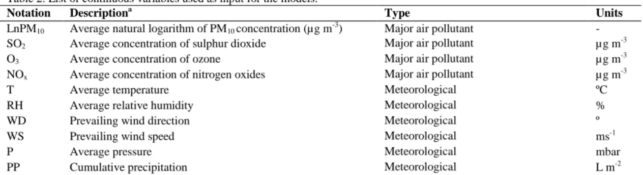
Table 2. List of continuous variables used as input for the models.
Notation Descriptiona Type Units
LnPM10 Average natural logarithm of PM10 concentration (µg m-3) Major air pollutant
-SO2 Average concentration of sulphur dioxide Major air pollutant µg m-3
O3 Average concentration of ozone Major air pollutant µg m-3
NOx Average concentration of nitrogen oxides Major air pollutant µg m-3
T Average temperature Meteorological ºC
RH Average relative humidity Meteorological %
WD Prevailing wind direction Meteorological º
WS Prevailing wind speed Meteorological ms-1
P Average pressure Meteorological mbar
PP Cumulative precipitation Meteorological L m-2
a Average values were calculated according to the corresponding duration of the PM10 sampling periods
table
Table 3. Statistical parameters used for evaluating the model performance
Evaluation Statistic Equation
EU Uncertainty Relative maximum error without timing
Relative directive error
Mean concentration Fractional bias
Performance
Correlation coefficient
Root mean square error
Normalised mean square error Fractional variance
RME = max CO,p-CE,p CO,p
RDE = CO,LV-CE,LV LV
FB = C - CO E 0.5 C + CO E r = CO,i - C CO E,i - C E n i=1 σOσE RMSE = 1 N CO,i-CE,i 2 N i=1 NMSE = CO- CE 2 CO C E FV = 2 σO-σE σO+ σE table
Table 4. Training and external validation performance indices of the various developed models at the Castro Urdiales site
a
T: Training; V: External validation b O: Observed; E: Estimated c Not calculated (n.c.) Pollutant Model Subseta
EU Uncertainty Mean Concentrationb Performance
RME (%) RDE (%) CO 10 2 C E 102 FB 102 r RMSE 102 NMSE 10 FV 10 Pb PLSR T 26.7 0.09 2.79 2.79 -9.8 10 -15 0.704 1.77 4.04 3.48 V 49.6 0.71 4.13 3.01 31.4 0.620 2.71 5.90 7.44 ANN T 34.5 0.66 2.67 2.70 -0.9 0.820 1.44 2.88 1.98 V 32.0 1.76 4.34 3.48 22.0 0.676 2.41 3.85 2.47 PCA-ANN T 36.9 0.41 3.14 3.11 1.0 0.681 2.03 4.25 4.41 V 30.6 0.07 3.08 3.43 -10.8 0.269 2.60 6.41 3.60 As PLSR T 42.8 0.30 6.66 6.66 -4.2 10 -12 0.656 5.17 6.02 4.16 V 34.8 1.74 5.32 5.50 -3.4 0.629 4.63 7.34 0.88 ANN T 77.0 0.17 6.96 6.81 2.1 0.130 6.96 10.22 12.74 V 66.3 0.25 5.32 6.81 -24.6 0.193 5.70 8.99 11.26 PCA-ANN T 54.6 0.86 6.96 6.35 9.1 0.536 5.87 7.80 7.36 V 33.5 0.96 5.55 6.33 -13.3 0.190 5.72 9.30 2.77 Ni PLSR T 34.7 10.83 27.61 27.61 3.1 10 -13 0.642 21.52 6.07 4.36 V 22.1 2.64 18.91 22.67 -18.1 0.663 12.27 3.51 -0.97 ANN T 45.0 6.19 28.27 23.30 19.3 0.676 21.59 7.08 6.18 V 32.6 1.24 19.36 23.71 -20.0 0.387 16.15 5.67 -0.58 PCA-ANN T 33.9 1.77 24.54 26.01 -5.8 0.643 17.60 4.85 4.92 V 25.6 2.06 23.64 23.42 0.9 0.216 21.19 8.11 1.64 Cd PLSR T 40.9 0.14 3.75 3.75 -1.1 10 -12 0.672 3.36 8.03 3.92 V 46.2 0.86 4.55 3.52 25.6 0.628 3.42 7.30 4.69 ANN T n.c. c n.c.c n.c.c n.c.c n.c.c n.c.c n.c.c n.c.c n.c.c V n.c.c n.c.c n.c.c n.c.c n.c.c n.c.c n.c.c n.c.c n.c.c PCA-ANN T 33.5 0.47 3.84 3.88 -1.1 0.613 3.11 6.49 5.36 V 41.5 0.42 3.56 3.62 -1.7 0.534 3.11 7.48 5.05 table
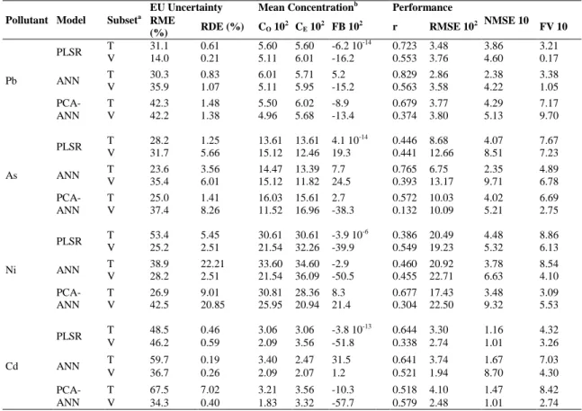
Table 5. Training and external validation performance indices of the various developed models at the Reinosa site
a
T: Training; V: External validation b O: Observed; E: Estimated Pollutant Model Subseta
EU Uncertainty Mean Concentrationb Performance
RME (%) RDE (%) CO 10 2 C E 102 FB 102 r RMSE 102 NMSE 10 FV 10 Pb PLSR T 31.1 0.61 5.60 5.60 -6.2 10 -14 0.723 3.48 3.86 3.21 V 14.0 0.21 5.11 6.01 -16.2 0.553 3.76 4.60 0.17 ANN T 30.3 0.83 6.01 5.71 5.2 0.829 2.86 2.38 3.38 V 35.9 1.07 5.11 5.95 -15.2 0.563 3.58 4.22 1.05 PCA-ANN T 42.3 1.48 5.50 6.02 -8.9 0.679 3.77 4.29 7.17 V 42.2 1.38 4.96 5.68 -13.4 0.374 3.80 5.13 9.70 As PLSR T 28.2 1.25 13.61 13.61 4.1 10 -14 0.446 8.68 4.07 7.67 V 31.7 5.66 15.12 12.46 19.3 0.441 12.66 8.51 7.23 ANN T 23.6 3.56 14.47 13.39 7.7 0.765 6.75 2.35 4.89 V 35.4 6.01 15.12 11.82 24.5 0.393 13.17 9.71 6.78 PCA-ANN T 25.0 1.41 16.03 15.61 2.7 0.572 10.03 4.02 6.69 V 37.4 8.26 11.52 16.96 -38.3 0.132 10.09 5.21 2.75 Ni PLSR T 53.4 5.45 30.61 30.61 -3.9 10 -6 0.386 20.49 4.48 8.86 V 25.2 2.51 21.54 32.26 -39.9 0.549 19.23 5.32 6.13 ANN T 38.9 22.21 33.60 34.60 -2.9 0.460 20.92 3.78 8.54 V 28.2 2.51 21.54 36.09 -50.5 0.455 22.71 6.63 4.10 PCA-ANN T 26.9 9.01 30.81 28.36 8.3 0.677 17.43 3.48 3.09 V 42.5 20.85 25.95 20.94 21.4 0.304 22.50 9.32 5.53 Cd PLSR T 48.5 0.46 3.06 3.06 -3.8 10 -13 0.644 3.30 1.16 4.32 V 46.2 0.59 2.09 3.56 -51.8 0.338 2.74 1.01 3.26 ANN T 59.7 0.19 3.40 2.47 31.5 0.641 3.74 1.67 7.03 V 36.7 0.26 2.09 2.07 1.2 0.521 1.94 8.70 4.30 PCA-ANN T 67.5 7.02 3.21 3.56 -10.3 0.518 4.10 1.47 8.42 V 34.3 0.40 1.83 3.32 -57.7 0.579 2.48 1.01 2.74 table